C A R F W o r k i n g P a p e r
CARF is presently supported by Bank of Tokyo-Mitsubishi UFJ, Ltd., Citigroup, Dai-ichi Mutual Life Insurance Company, Meiji Yasuda Life Insurance Company, Nippon Life Insurance Company, Nomura Holdings, Inc. and Sumitomo Mitsui Banking Corporation (in alphabetical order). This financial support enables us to issue CARF Working Papers.
CARF Working Papers can be downloaded without charge from: http://www.carf.e.u-tokyo.ac.jp/workingpaper/index.cgi
Working Papers are a series of manuscripts in their draft form. They are not intended for circulation or distribution except as indicated by the author. For that reason Working Papers may not be reproduced or distributed without the written consent of the author.
CARF-F-230
Modeling of Interest Rate Term Structures under
Collateralization and its Implications
Masaaki Fujii The University of Tokyo
Akihiko Takahashi The University of Tokyo First Version: September 2010 Current Version: December 2010
Modeling of Interest Rate Term Structures under
Collateralization and its Implications
∗Masaaki Fujii†, Akihiko Takahashi‡ First version: 22 September 2010 Current version: 22 December 2010
Abstract
In recent years, we have observed dramatic increase of collateralization as an im-portant credit risk mitigation tool in over the counter (OTC) market [6]. Combined with the significant and persistent widening of various basis spreads, such as Libor-OIS and cross currency basis, the practitioners have started to notice the importance of difference between the funding cost of contracts and Libors of the relevant currencies. In this article, we integrate the series of our recent works [1, 2, 4] and explain the consistent construction of term structures of interest rates in the presence of collat-eralization and all the relevant basis spreads, their no-arbitrage dynamics as well as their implications for derivative pricing and risk management. Particularly, we have shown the importance of the choice of collateral currency and embedded ”cheapest-to-deliver” (CTD) option in a collateral agreement.
Keywords : swap, collateral, Libor, OIS, EONIA, Fed-Fund, cross currency, basis, HJM, CSA, CVA
∗Forthcoming inProceedings of KIER-TMU International Workshop on Financial Engineering, 2010. This research is supported by CARF (Center for Advanced Research in Finance) and the global COE program“The research and training center for new development in mathematics.”M.Fujii and A.Takahashi are grateful for Yasufumi Shimada, a manager of Shisei Bank, and also for Fujii’s former colleagues of Morgan Stanley, especially in IDEAS, IR option, and FX Hybrid desks in Tokyo for fruitful and stimulating discussions. The contents of the paper do not represent any views or opinions of Morgan Stanley nor Shinsei Bank. The authors are not responsible or liable in any manner for any losses and/or damages caused by the use of any contents in this research.
†Graduate School of Economics, The University of Tokyo. ‡Graduate School of Economics, The University of Tokyo
1
Introduction
The recent financial crisis and the following liquidity and credit squeeze have caused
signif-icant and persistent widening of various basis spreads1. In particular, we have witnessed
drastic movement of cross currency swap (CCS), Libor-OIS, and tenor swap2 (TS) basis
spreads. In some occasions, the size of spreads has exceeded several tens of basis points, which is far wider than the general size of bid/offer spreads. Furthermore, there has been a dramatic increase of collateralization in financial contracts recent years, and it has be-come almost a market standard among the major financial institutions, at least [6]. The importance of the collateralization is mainly twofold: 1) reduction of the counterparty credit risk, and 2) change of the funding cost of the trade. The first one is well recognized, and there exist a large number of studies in the context of credit value adjustment (CVA). Although it is not as obvious as the first one, the second effect is also important and it has started to attract strong attentions among practitioners.
As we will see later, the details of collateralization specified in CSA (credit support annex), the existence of various basis spreads change the effective discounting rate appro-priate for the specific contract. Because of the characteristic of the products, the effects are most relevant in interest rate and long-dated foreign exchange (FX) markets. These findings cast a strong warning to the financial institutions using the standard Libor Mar-ket Model (LMM), which treats the Libor as a risk-free interest rate and hence cannot reflect the existence of various basis spreads and collateralization. These drawbacks make the LMM incapable of calibrating to the relevant swap markets nor their dynamics, which is likely to cause the financial firms overlooking critical risk exposures.
In this article, we provide a systematic solution for the above market developments by integrating our series works, Fujii, Shimada & Takahashi (2009, 2009, 2010) [1, 2, 4]. We first present the pricing formula of derivatives under the collateralization, including the case where the payment and collateral currencies are different. Based on this result, we propose the procedures for the consistent term structure construction of collateralized swaps in multi-currency environment. Secondly, we provide the no-arbitrage dynamics under Heath-Jarrow-Morton (HJM) framework which is capable of calibrating to all the relevant swaps and allow full stochastic modeling of basis spreads. Thirdly, we explain the importance of the choice of collateral currency and the effects of embedded ”cheapest-to-deliver” option in collateral agreement when it allows the replacement of collateral currency. And then, we conclude.
As related works, we refer to Johannes & Sundaresan (2007) [7] (and its working paper) as the first work focusing on the cost of collateral posting and studying its effect on the swap par rates based on empirical analysis of the US treasury and swap markets. More recently, Piterbarg (2010) [8] has used the similar formula given in [7] to take the collateral cost into account for the option pricing in general, but he has not discussed the case where the payment and collateral currencies are different, nor the term structure modeling of interest rate and FX under the collateralization.
1
A basis spread generally means the interest rate differentials between two different floating rates. 2
It is a floating-vs-floating swap that exchanges Libors with two different tenors with a fixed spread in one side.
2
Pricing under the collateralization
This section reviews [1], our results on pricing derivatives under the collateralization. Let us make the following simplifying assumptions about the collateral contract.
1. Full collateralization (zero threshold) by cash.
2. The collateral is adjusted continuously with zero minimum transfer amount.
In fact, the daily margin call is now quite popular in the market and there is also an increasing tendency to include a provision for ”add-hoc call”, which allows the participants to call margin arbitrary time in addition to the periodical regular calls. Furthermore, there is a wide movement to reduce the threshold and minimum transfer amount since the various studies indicate that the existence of meaningful size of these variables significantly reduces the effectiveness of credit risk mitigation of collateralization, which results in higher CVA charge in turn. These developments make our assumptions a good proxy for the market reality at least for the standard fixed income products. Since the assumptions allow us to neglect the loss given default of the counterparty, we can treat each trade/payment separately without worrying about the non-linearity arising from the netting effects and the asymmetric handling of exposure.
We consider a derivative whose payoff at timeT is given byh(i)(T) in terms of currency
”i”. We suppose that the currency ”j” is used as the collateral for the contract. Note
that the instantaneous return (or cost when it is negative ) by holding the cash collateral at time tis given by
y(j)(t) =r(j)(t)−c(j)(t) , (2.1)
where r(j) and c(j) denote the risk-free interest rate and collateral rate of the currency j, respectively. In the case of cash collateral, the collateral rate c(i) is usually given by the overnight rate of the corresponding currency, such as Fed-Fund rate for USD. If we denote the present value of the derivative at time t by h(i)(t) (in terms of currency i),
the collateral amount posted from the counterparty is given by
(
h(i)(t)/fx(i,j)(t)
)
, where
fx(i,j)(t) is the foreign exchange rate at timetrepresenting the price of the unit amount of
currency j in terms of currency i. These considerations lead to the following calculation
for the collateralized derivative price,
h(i)(t) = EQi t [ e−∫tTr (i)(s)ds h(i)(T) ] + fx(i,j)(t)EQj t [∫ T t e−∫tsr(j)(u)duy(j)(s) ( h(i)(s) fx(i,j)(s) ) ds ] , (2.2) where EQi
t [·] is the time tconditional expectation under the risk-neutral measure of
cur-rencyi, where the money-market account of currencyiis used as the numeraire. Here, the
second term takes into account the return/cost from holding the collateral. By aligning
the measure to Qi, we obtain
h(i)(t) =EQi t [ e− ∫T t r(i)(s)dsh(i)(T) + ∫ T t e− ∫s t r(i)(u)duy(j)(s)h(i)(s)ds ] . (2.3)
Now, it is easy to see that X(t) :=e− ∫t 0r (i)(s)ds h(i)(t) + ∫ t 0 e− ∫s 0 r (i)(u)du y(j)(s)h(i)(s)ds (2.4) is aQi-martingale under appropriate integrability conditions. This tells us that the process
of the option value can be written as
dh(i)(t) =
(
r(i)(t)−y(j)(t)
)
h(i)(t)dt+dM(t) (2.5)
with some Qi-martingaleM.
As a result, we have the following theorem:
Theorem 1 3 Suppose thath(i)(T)is a derivative’s payoff at timeT in terms of currency ”i” and that the currency ”j” is used as the collateral for the contract. Then, the value of the derivative at time t, h(i)(t) is given by
h(i)(t) = EQi t [ e−∫tTr (i)(s)ds( e∫tTy (j)(s)ds) h(i)(T) ] (2.6) = D(i)(t, T)ET c (i) t [ e−∫tTy (i,j)(s)ds h(i)(T) ] , (2.7) where y(i,j)(s) =y(i)(s)−y(j)(s) (2.8)
with y(i)(s) = r(i)(s)−c(i)(s) and y(j)(s) = r(j)(s)−c(j)(s). Here, we have also defined the collateralized zero-coupon bond of currency ias
D(i)(t, T) =EQi t [ e−∫tTc (i)(s)ds] (2.9)
and the collateralized forward measure Tc
(i), where the collateralized zero-coupon bond is
used as the numeraire; thus, ET c
(i)
t [·] denotes the time t conditional expectation under the
measure T(ci).
As a corollary of the theorem, we have
h(t) = EtQ
[
e−∫tTc(s)dsh(T) ]
= D(t, T)EtTc[h(T)] (2.10)
when the payment and collateral currencies are the same.
Finally, let us also define the forward collateral rate of currency i, c(i)(t, T), for the
convenience of later discussion:
c(i)(t, T) =− ∂ ∂T lnD (i)(t, T) , (2.11) or equivalently D(i)(t, T) = exp ( − ∫ T t c(i)(t, s)ds ) . (2.12) 3
Although we are dealing with continuous processes here, we obtain the same result as long as there is no simultaneous jump of underlying assets when the counterparty defaults even in more general setting.
3
Calibration to Single Currency Swaps
In this section, we construct the relevant yield curves in a single currency market, where there exist three different types of interest rate swap, which are overnight index swap (OIS), standard interest rate swap (IRS), and tenor swap (TS). In the following, we explain how we can extract relevant forwards based on the result of previous section following the works [1, 3, 4]. Throughout this section, we assume that the relevant swap is collateralized by the domestic (or payment) currency.
3.1 Overnight Index Swap
As we have seen in the previous section, it is critical to determine the forward curve of overnight rate for the pricing of collateralized swaps. Fortunately, there is a product called ”overnight index swap” (OIS), which exchanges the fixed coupon and the daily-compounded overnight rate. Here, let us assume that the OIS itself is continuously collat-eralized by the domestic currency. In this case, using the Eq.(2.10), we get the consistency condition of T0-start TN-maturing OIS rate as
OISN N ∑ n=1 ∆nEQ [ e−∫0Tnc(s)ds ] = N ∑ n=1 EtQ [ e−∫0Tnc(s)ds ( e ∫Tn Tn−1c(s)ds−1 )] . (3.1)
Here, OISN is the market quote of par rate for the length-N OIS, andc(t) is the overnight
(and hence collateral) rate at time t of the domestic currency. ∆ and δ denote day-count
fractions for fixed and floating legs, respectively. We can simplify the above equation into the form OISN N ∑ n=1 ∆nD(0, Tn) =D(0, T0)−D(0, TN) (3.2)
by using the collateralized zero-coupon bond. Now, from Eq.(3.2), we can easily obtain
the term structure ofD(0,·) by the standard bootstrap and spline techniques [5].
3.2 Interest rate swap
In the standard interest rate swap (IRS), two parties exchange a fixed coupon and Libor
for a certain period with a given frequency. The tenor of Libor ”τ” is determined by the
frequency of floating payments, i.e., 6m-tenor for semi-annual payments, for example. For
a T0-startTM-maturing IRS with the Libor of tenorτ, we have
IRSM M ∑ m=1 ∆mD(0, Tm) = M ∑ m=1 δmD(0, Tm)ET c m[L(T m−1, Tm;τ)] (3.3)
as a consistency condition. Here, IRSM is the market IRS quote, L(Tm−1, Tm;τ) is the
Libor rate with tenor τ for a period of (Tm−1, Tm). Since we already have the term
structure of D(0,·), it is straightforward to extract the set of ETmc[L(T
m−1, Tm;τ)] for
3.3 Tenor swap
A tenor swap is a floating-vs-floating swap where the parties exchange Libors with different tenors with a fixed spread on one side, which we call TS basis spread in this article. Usually, the spread is added on top of the Libor with shorter tenor. For example, in a 3m/6m tenor swap, quarterly payments with 3m Libor plus spread are exchanged by semi-annual payments of 6m Libor flat. The condition that the tenor spread should satisfy is N ∑ n=1 δnD(0, Tn) ( ETnc[L(T n−1, Tn;τS)] + TSN ) = M ∑ m=1 δmD(0, Tm)ET c m[L(T m−1, Tm;τL)] , (3.4)
where TN = TM, ”m” and ”n” distinguish the difference of payment frequency. TSN
denotes the market quote of of the basis spread for the T0-start TN-maturing tenor swap.
The spread is added on the Libor with the shorter tenorτS in exchange for the Libor with
longer tenorτL. From the above relation, one can extract the forward Libor with different
tenors.
Here, we have explained using slightly simplified terms of contract. In the actual mar-ket, it is more common that the coupons of the Leg with the shorter tenor are compounded by Libor flat and being paid with the same frequency of the other Leg. However, the size of correction from the above simplification can be shown negligibly small.
3.4 Calibration Example
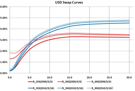
Figure 1: USD zero rate curves of Fed-Fund rate, 3m and 6m Libors.
In Fig. 1, we have given examples of calibrated yield curves for USD market on
2009/3/3 and 2010/3/16, where ROIS,R3m and R6m denote the zero rates for OIS
−ln(D(0, T))/T. For the forward Libor, the zero-rate curve Rτ(·) is determined
recur-sively through the relation
ETmc[L(T m−1, Tm;τ)] = 1 δm ( e−Rτ(Tm−1)Tm−1 e−Rτ(Tm)Tm −1 ) . (3.5)
In the actual calculation of D(0,·), we have used the Fed-Fund vs 3m-Libor basis swap,
where the two parties exchange 3m Libor and the compounded Fed-Fund rate with spread, which seems more liquid and a larger number of quotes available than the usual OIS. In Fig. 2, one can see the historical behavior of the spread between 1yr IRS and OIS for USD, JPY and EUR, where the underlying floating rates of IRS are 3m-Libor for USD and EUR and 6m-Libor for JPY.
Figure 2: Difference between 1yr IRS and OIS. Underlying floating rates are 3m-Libor for USD and EUR, and 6m-Libor for JPY.
Remarks: In the above calculations, we have assumed that the conditions given in the previous section are satisfied, and also that all the instruments are collateralized by the cash of domestic currency which is the same as the payment currency. Cautious readers may worry about the possibility that the market quotes contain significant contributions from market participants who use a foreign currency as collateral. However, the induced changes in IRS/TS quotes are very small and impossible to distinguish from the bid/offer spreads in normal circumstances, because the correction appears both in the fixed and
floating legs which keeps the market quotes almost unchanged 4. However, as we will
see in the later sections, the present values of off-the-market swaps will be significantly affected when the collateral currency is different.
4
As for cross currency swaps, the change can be a few basis point, and hence comparable to the market bid/offer spreads.
4
Calibration to Cross Currency Swaps
After completing the calibration to the single currency swaps, we should have obtained the terms structures of D(i)(0, T) and ET(ci)[L(i)(T
m−1, Tm;τ) ]
for each currency and tenor.
The remaining freedom of the model is the term structure of y(i,j)(·) for each relevant
currency pair. As we will see, this is the most important ingredient to determine the value of CCS.
4.1 Mark-to-Market Cross Currency Swap
In this section, we will discuss how to make the term structure consistent with CCS (cross currency swap) markets [1, 3]. The current market is dominated by USD crosses where 3m USD Libor flat is exchanged with 3m Libor of a different currency with additional basis spread. There are two types of CCS, one is CNCCS (Constant Notional CCS), and the other is MtMCCS (Mark-to-Market CCS). In a CNCCS, the notionals of both legs are fixed at the inception of the trade and kept constant until its maturity. On the other hand, in a MtMCCS, the notional of USD leg is reset at the start of every calculation period of the Libor while the notional of the other leg is kept constant throughout the contract period. Although the required calculation becomes a bit more complicated, we
will use MtMCCS for calibration due to its better liquidity5.
First, let us definey(i,j)(t, s), the forward rate ofy(i,j)(s) at timet as
e−∫tTy (j,i)(t,s)ds =EQj t [ e−∫tTy (j,i)(s)ds] . (4.1)
We consider a MtMCCS of (i, j) currency pair, where the leg of currency i (intended to
be USD) needs notional refreshments. We assume that the collateral is posted in currency
i, which seems common in the market. The value of j-leg of a T0-start TN-maturing
MtMCCS is calculated as P Vj = −D(j)(0, T0)ET c 0,(j) [ e−∫0T0y(j,i)(s)ds ] +D(j)(0, TN)ET c n,(j) [ e−∫0TNy(j,i)(s)ds ] + N ∑ n=1 δ(nj)D(j)(0, Tn)ET c n,(j) [ e−∫0Tny (j,i)(s)ds( L(j)(Tn−1, Tn;τ) +BN )] , (4.2)
where the basis spreadBN is available as a market quote. In [2], we have assumed that all
of the{y(k)(·)}and hence {y(i,j)(·)} are deterministic functions of time to make the curve construction more tractable. Here, we slightly relax the assumption allowing randomness of {y(i,j)(·)}. As long as we assume that {y(i,j)(·)} is independent from the dynamics of Libors and collateral rates, the procedures of bootstrapping given in [2] can be applied in
the same way 6. Under the assumption of independence, we obtain
P Vj = −D(j)(0, T0)e− ∫T0 0 y(j,i)(0,s)ds+D(j)(0, T N)e− ∫TN 0 y(j,i)(0,s)ds + N ∑ n=1 δn(j)D(j)(0, Tn)e− ∫Tn 0 y (j,i)(0,s)ds( ETn,c(j)[L(j)(T n−1, Tn;τ)] +BN ) .(4.3) 5
As for the details of MtMCCS and CNCCS, see [1, 3]. 6
In practice, it would not be a problem even if there is a non-zero correlation as long as it does not meaningfully change the model implied quotes compared to the market bid/offer spreads.
On the other hand, the present value ofi-leg in terms of currencyj is given by P Vi = − N ∑ n=1 EQi [ e− ∫Tn−1 0 c(i)(s)dsf(i,j) x (Tn−1) ] /fx(i,j)(0) + N ∑ n=1 EQi [ e−∫0Tnc (i)(s)ds fx(i,j)(Tn−1) ( 1 +δ(ni)L(i)(Tn−1, Tn;τ) )] /fx(i,j)(0) = N ∑ n=1 δ(ni)D(i)(0, Tn)ET c n,(i) [ fx(i,j)(Tn−1) fx(i,j)(0) B(i)(Tn−1, Tn;τ) ] , (4.4) where B(i)(t, Tk;τ) =E Tc k,(i) t [ L(i)(Tk−1, Tk;τ) ] − 1 δk(i) ( D(i)(t, Tk−1) D(i)(t, T k) −1 ) , (4.5)
which represents a Libor-OIS spread. Since we found no persistent correlation between FX and Libor-OIS spread in historical data, we have treated them as independent variables. Even if a non-zero correlation exists in a certain period, the expected correction seems not numerically important due to the typical size of bid/offer spreads for MtMCCS (about a few bps at the time of writing). Since 3-month timing adjustment of FX is safely negligible,
an approximate value ofi-leg is obtained as
P Vi≃ N ∑ n=1 δn(i)D(i)(0, Tn) D(j)(0, Tn−1) D(i)(0, T n−1) e− ∫Tn−1 0 y(j,i)(0,s)dsB(i)(0, Tn;τ). (4.6)
Here, we have used the following expression of the forward FX collateralized with currency
i: fx(i,j)(t, T) =fx(i,j)(t)D (j)(t, T) D(i)(t, T)e −∫T t y (j,i)(t,s)ds . (4.7)
Notice that, after calibrating to the single currency swaps for each currency, the only
unknown in Eqs. (4.3) and (4.6) is y(j,i)(0,·). Therefore, one can easily see that the
consistency condition P Vi =P Vj with given market spread BN for each maturity allows
us to bootstrap the term structure of {y(i,j)(0,·)}. Finally, let us mention the fact that
the (i, j)-MtMCCS par spread is expressed as
BN = N ∑ n=1 δ(ni)D(Ti) n D (j) Tn−1 DT(i) n−1 e−∫0Tn−1y(j,i)(0,s)dsB(i) Tn− N ∑ n=1 δn(j)D(Tj) ne −∫Tn 0 y (j,i)(0,s)ds BT(j) n − N ∑ n=1 DT(j) n−1e −∫Tn−1 0 y(j,i)(0,s)ds ( e− ∫Tn Tn−1y (j,i)(0,s)ds −1 )] / N ∑ n=1 δ(nj)DT(j) ne −∫Tn 0 y (j,i)(0,s)ds , (4.8) in the above mentioned approximation, where we have shortened the notations asD(k)(0, T) =
4.2 Calibration Example and Historical Behavior
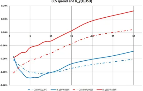
In Fig. 3, we have given examples of calibration for EUR/USD and USD/JPY MtMCCS as of 2010/3/16. We have plotted the zero rates ofy(j,i) defined as
Ry(j,i)(T) =− ln ( EQj [ e−∫0Ty (j,i)(s)ds]) T = 1 T ∫ T 0 y(j,i)(0, s)ds (4.9) together with the term structure of MtMCCS basis spreads. It is easy to expect that there are significant contributions from the second line of Eq. (4.8) to the CCS basis
spreads from the similarities between Ry(X,U SD) and CCS quotes. The implied forward
FXs derived from Eq. (4.7) were well within the bid/offer spreads7.
Figure 3: MtMCCS par spreads,Ry(J P Y,U SD) and Ry(EU R,U SD) as of 2010/3/16.
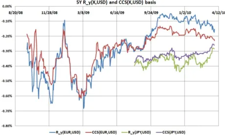
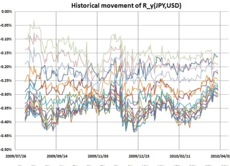
Let us also check the historical behavior of Ry(EU R,U SD) and Ry(J P Y,U SD) given in
Fig. 4 to 8 8. For both cases, the term structures of Ry have quite similar shapes and
levels to those of the corresponding CCS basis spreads. In Fig. 4, historical behavior of
Ry(X,U SD)(T = 5y) (X= EUR, JPY ) and corresponding 5y-MtMCCS spreads are given.
One can see that a significant portion of CCS spreads movement stems from the change of y(i,j), rather than the difference of Libor-OIS spread between two currencies. The level (difference)-correlation between Ry and CCS spread is quite high, which is about 93% (69%) for EUR or about 70% (48%) for JPY for the historical series used in the figure, for example.
The 3m-roll historical volatilities of y(EU R,U SD) instantaneous forwards, which are
annualized in absolute terms, are given in Fig. 9. In a calm market, they tend to be 50 bps or so, but they were more than a percentage point just after the market crisis,
7
In any case, it is quite wide for long maturities. 8
Due to the lack of OIS data for JPY market, we have only a limited data for (JPY,USD) pair. We have used Cubic Monotone Spline for calibration although the figures are given in linear plots for ease. For spline technique, see [5], for example.
Figure 4: Ry(EU R,U SD)(5y),Ry(J P Y,SD)(5y) and corresponding quotes of 5y-MtMCCS.
which is reflecting a significant widening of the CCS basis spread to seek USD cash in the
low liquidity market. Except the CCS basis spread, y does not seem to have persistent
correlations with other variables such as OIS, IRS and FX forwards. At least, within our limited data, the 3m-roll historical correlations with these variables fluctuate mainly
around ±20% or so.
5
No-arbitrage dynamics in Heath-Jarrow-Morton
Frame-work
In this section, we give the set of SDEs for the whole system 9. From the previous
discussion, we have seen that the relevant building blocks of term structures are given by {D(i)(t, T)}, {ET c n,(i) t [ L(i)(Tn−1, Tn;τ) ] }, and {y(i,j)(t, T)} , (5.1) or equivalently {c(i)(t, T)}, {B(i)(t, T;τ)}, and {y(i,j)(t, T)} , (5.2) for each maturity T, tenor τ, currency i, and currency pair (i, j). As seen in Sec.2, the collateral rate plays a critical role as the effective discounting rate. Thus, let us fix the base currencyi, and consider the dynamics ofc(i)(t, s). Suppose that the dynamics of the
forward collateral rate under the Qi is given by
dc(i)(t, s) =α(i)(t, s)dt+σ(ci)(t, s)·dWQi(t) , (5.3)
where α(i)(t, s) is a scalar function for its drift, and WQi(t) is a d-dimensional
Brown-ian motion under the Qi-measure. σc(i)(t, s) is a d-dimensional vector and the following 9See [2, 3, 4] for details.
abbreviation have been used: σc(i)(t, s)·dWQi(t) = d ∑ j=1 [ σ(ci)(t, s) ] jdW Qi j (t). (5.4)
Here, we will not specify the details of the volatility process : It can depend on the collateral rate itself, or any other state variables.
Applying Itˆo’s formula to Eq.(2.12), we have
dD(i)(t, T) D(i)(t, T) = { c(i)(t)− ∫ T t α(i)(t, s)ds+1 2 ∫tT σc(i)(t, s)ds 2} dt− (∫ T t σc(i)(t, s)ds ) ·dWQi t . (5.5) On the other hand, by definition, the drift rate of D(i)(t, T) should bec(i)(t) =c(i)(t, t).
Therefore, it is necessary that
α(i)(t, s) = d ∑ j=1 [σ(ci)(t, s)]j (∫ s t σ(ci)(t, u)du ) j (5.6) = σ(ci)(t, s)· (∫ s t σ(ci)(t, u)du ) , (5.7)
and as a result, the process of c(i)(t, s) under theQi-measure is given by
dc(i)(t, s) =σ(ci)(t, s)· (∫ s t σ(ci)(t, u)du ) dt+σ(ci)(t, s)·dWQi(t) . (5.8)
In exactly the same way, we obtain
dy(i,j)(t, s) =σy(i,j)(t, s)· (∫ s t σ(yi,j)(t, u)du ) dt+σy(i,k)(t, s)·dWQi(t) . (5.9)
Next, let us consider the dynamics of Libor-OIS spread, B(i)(t, T;τ). From the def-inition in Eq. (4.5), it is clear that B(i)(·, T;τ) is a martingale under the collateralized
forward measure Tc
(i), where the numeraire is given byD(i)(·, T). Using the
Maruyama-Girsanov theorem, one can see that Brownian motion under the forward measureT(ci), or
WT(ci), is related to theWQi as dWT(ci)(t) = (∫ T t σ(ci)(t, s)ds ) dt+dWQi(t) , (5.10)
and hence, one easily obtains
dB(i)(t, T;τ) B(i)(t, T;τ) =σ (i) B (t, T;τ)· (∫ T t σc(i)(t, s)ds ) dt+σB(i)(t, T;τ)·dWQi(t) . (5.11)
Since we have the relation
the SDE for the spot FX process is given by dfx(i,j)(t)/fx(i,j)(t) = ( c(i)(t)−c(j)(t) +y(i,j)(t) ) dt+σX(i,j)(t)·dWQi(t). (5.13)
Maruyama-Girsanov theorem tells us that Brownian motions in two different currencies are related by the formula
dWQj(t) =−σ(i,j)
X (t)dt+dWQi(t), (5.14)
which allows us to derive the SDEs of these building blocks under a different base currency,
too. For example, the SDE of collateral rate of the foreign currency j is given by
dc(j)(t, s) =σc(j)(t, s)· [(∫ s t σc(j)(t, u)du ) −σ(Xi,j)(t) ] dt+σc(j)(t, s)·dWQi(t) . (5.15)
Pricing formulas for some of the vanilla options are available in [2].
6
Implications for Derivative Pricing
Although it is worth exploring various implications of collateralization by using the dy-namics given in the previous section, the leading order effects are expected to arise from the change of the effective discounting rate. In this section, we discuss some of these important implications by using the calibrated yield curves.
6.1 Choice of Collateral Currency
When the payment and collateral currencies are the same, the discounting factor is given by the collateral rate which is under control of the relevant central bank as indicated in Eq. (2.10). Traditionally, among financial firms, the Libor curve has been widely used to discount the future cash flows. However, this method would easily underestimate their values by several percentage points for long maturities, even with the current level of
Libor-OIS spread, or 10∼20 bps. Considering the mechanism of collateralization, financial firms
need to hedge the change of OIS in addition to the standard hedge against the movement of Libors. Especially, the risk of floating-rate payments needs to be checked carefully, since the overnight rate can move in the opposite direction to the Libor as was observed in this financial crisis. In Fig. 10, the present values of Libor floating legs with final principal (= 1) payment P V = N ∑ n=1 δnD(0, Tn)ET c n[L(T n−1, Tn;τ)] +D(0, TN) (6.1)
are given for various maturities. If traditional Libor discounting is being used, the stream of Libor payments has the constant present value ”1”, which is obviously wrong from our results. This point is very important in risk-management, since financial firms may overlook the quite significant interest-rate risk exposure when they adopt the traditional interest rate model in their system.
If a trade with payment currencyjis collateralized by foreign currencyi, an additional
modification to the discounting factor appears ( See, Eq. (4.1).) 10:
e−∫tTy (j,i)(t,s)ds =EQj t [ e−∫tTy (j,i)(s)ds] . (6.2)
From Figs. 6 and 8, one can see that posting USD as collateral tends to be expensive from the view point of collateral payers, which is particularly the case when the market is illiquid. For example, from Fig. 8, one can see that the value of JPY payment in 10 years time is more expensive by around 3% when it is collateralized by USD instead of JPY. The effects should be more profound for emerging currencies where the implied CCS basis spread can easily be 100 bps or more.
6.2 Embedded Cheapest-to-Deliver Option
We now discuss the embedded CTD option in a collateral agreement. In some cases, financial firms make contracts with CSA allowing several currencies as eligible collateral. Suppose that the payer of collateral has a right to replace a collateral currency whenever he wants. If this is the case, the collateral payer should choose the cheapest collateral currency to post, which leads to the modification of the discounting factor as
EQj t [ e−∫tTmaxi∈C{y (j,i)(s)}ds] , (6.3)
where C is the set of eligible currencies. Note that, by the definition of collateral payers,
they want to make (−P V) (> 0) as small as possible. Although there is a tendency
toward a CSA allowing only one collateral currency to reduce the operational burden, it does not seem uncommon to accept the domestic currency and USD as eligible collateral, for example. In this case, the above formula turns out to be
EQj t [ e−∫tTmax{y (j,USD)(s),0}ds] . (6.4)
In Figs. 11 and 12, we have plotted the modifications of discounting factors given in
Eq. (6.4), for j = EUR and JPY as of 2010/3/16. We have used the Hull-White model
for the dynamics of y(EU R,U SD)(·) and y(J P Y,U SD)(·), with a mean reversion parameter
1.5% per annum and the set of volatilities, σ = 0,25,50 and 75 bps 11, respectively. As
can be seen from the historical volatilities given in Fig. 9, σ can be much higher under
volatile environment. The curve labeled by USD (EUR, JPY) denotes the modification of the discount factor when only USD (EUR, JPY) is eligible collateral for the ease of comparison. One can easily see that there is significant impact when the collateral currency chosen optimally. For example, from Fig. 12, one can see if the parties choose the collateral currency from JPY and USD optimally, it roughly increases the effective discounting rate by around 50 bps annually even when the annualized volatility of spread y(J P Y,U SD) is 50 bps.
In the calculation, we have used daily-step Monte Carlo simulation. Although we can expect that there are various obstacles to implement the optimal strategy in practice, the development of common infrastructure for collateral management, such as the electronic automation of the margin call and collateral delivery, will make the optimal choice of collateral currency be an important issue in coming years.
10
Here, we are assuming independence ofyfrom reference assets. 11These are annualized volatilities in absolute terms.
7
Conclusions
In this article, which integrates the series of our recent works [1, 2, 4], we explain the consistent construction of multiple swap curves in the presence of collateralization and cross currency basis spreads, their no-arbitrage dynamics, and implications for derivative pricing. Especially, we have shown the importance of the choice of collateral currency and embedded ”cheapest-to-deliver” (CTD) option in collateral agreements. We have also emphasized dangers to use the standard LMM in actual financial business since it allows the financial firms to overlook potentially critical risk exposures.
References
[1] Fujii, M., Shimada, Y., Takahashi, A., 2009, ”A note on construction of multiple swap curves with and without collateral,” CARF Working Paper Series F-154, available at http://ssrn.com/abstract=1440633.
[2] Fujii, M., Shimada, Y., Takahashi, A., 2009, ”A Market Model of Interest Rates with Dynamic Basis Spreads in the presence of Collateral and Multiple Currencies”, CARF Working Paper Series F-196, available at http://ssrn.com/abstract=1520618.
[3] Fujii, M., Shimada, Y., Takahashi, A., 2010, ”On the Term Structure of Interest Rates with Basis Spreads, Collateral and Multiple Currencies”, based on the presentations given at ”International Workshop on Mathematical Finance” at Tokyo, Japanese Financial Service Agency, and Bank of Japan.
[4] Fujii, M., Shimada, Y., Takahashi, A., 2010, ”Collateral Posting and Choice of Col-lateral Currency-Implications for derivative pricing and risk management”, CARF Working Paper Series F-216, available at http://ssrn.com/abstract=1601866.
[5] Hagan, P.S. and West, G., 2006, ”Interpolation Methods for Curve Construction”, Applied Mathematical Finance, Vol. 13, No. 2, 89-126.
[6] ISDA Margin Survey 2010, Preliminary Results,
Market Review of OTC Derivative Bilateral Collateralization Practices, ISDA Margin Survey 2009.
[7] Johannes, M. and Sundaresan, S., 2007, ”The Impact of Collateralization on Swap Rates”, Journal of Finance 62, 383410.
[8] Piterbarg, V. , 2010, ”Funding beyond discounting : collateral agreements and deriva-tives pricing” Risk Magazine.
Figure 5: Historical movement of calibrated Ry(EU R,U SD).
Figure 7: Historical movement of calibratedRy(J P Y,U SD).
Figure 9: 3M-Roll historical volatility of y(EU R,U SD) instantaneous forward. Annualized in absolute terms.
Figure 11: Modification of EUR discounting factors based on HW model for y(EU R,U SD)
as of 2010/3/16. The mean-reversion parameter is 1.5%, and the volatility is given at each
label.
Figure 12: Modification of JPY discounting factors based on HW model fory(J P Y,U SD)as
of 2010/3/16. The mean-reversion parameter is 1.5%, and the volatility is given at each