Market Niching in Multi-attribute Computational Resource
Allocation Systems
Edward Robinson
School of Computer Science University of Birmingham, UKPeter McBurney
Department of Informatics King’s College London, UKXin Yao
School of Computer Science University of Birmingham, UK
ABSTRACT
We propose a novel method for allocating multi-attribute computational resources via competing marketplaces. Trad-ing agents, workTrad-ing on behalf of resource consumers and providers, choose to trade in resource markets where the re-sources being traded best align with their preferences and constraints. Market-exchange agents, in competition with each other, attempt to provide resource markets that attract traders, with the goal of maximising their profit. Because exchanges can only partially observe global supply and de-mand schedules, novel strategies are required to automate their search for market niches. Novel attribute-level selec-tion (ALS) strategies are empirically analysed in simulated competitive market environments, and results suggest that using these strategies, market-exchanges can seek out mar-ket niches under a variety of environmental conditions.
Categories and Subject Descriptors
I.2.11 [Artificial Intelligence]: Distributed Artificial Intel-ligence—Intelligent Agents, Multiagent systems;
J.4 [Social and Behavioural Sciences]: Economics
General Terms
Market-based Control, Double Auctions, Automated Market Niching
1.
INTRODUCTION
The significant growth of Internet-enabled devices is accom-panied by a continually increasing demand for access to computational resources and services, in order to satisfy an ever growing user base. This is resulting in current system-centric approaches to resource allocation becoming limit-ing [6]. Market-based approaches [4] have been suggested as a way to efficiently allocate distributed resources, e.g., computational resources, between competing self-interested agents. Computational resources are multi-attribute in na-ture, and may be described by, for example, their
compu-Permission to make digital or hard copies of all or part of this work for personal or classroom use is granted without fee provided that copies are not made or distributed for profit or commercial advantage and that copies bear this notice and the full citation on the first page. To copy otherwise, to republish, to post on servers or to redistribute to lists, requires prior specific permission and/or a fee.
ICEC11Liverpool, UK Copyright 2011 ACM ...$10.00.
tational power and storage capacity. Often, resources such as these are allocated either in a fully decentralised way, e.g., bargaining or Catallaxy approaches, or conversely a fully centralised approaches, e.g., multi-attribute or com-binatorial auctions; see [2] for an overview. There are sev-eral problems with these existing approaches. For example, fully decentralised approaches, while being robust to fail-ure, can suffer from inefficient allocations, either due to find-ing optimal tradfind-ing partners or the lack of a suitable price-discovery method. Fully centralised approaches, such as one-sided multi-attribute/combinatorial auctions, while offering economically efficient allocations are non-distributable and often the allocation process is computationally prohibitive [1].
One approach that has not received attention is to con-sider the allocation of multi-attribute resources via distributed competing market institutions. Using this approach, con-sumers and providers would have multiple double-auction market institutions available, to trade various types of com-putational resources. Traders within the system could choose to trade in the markets for resources that most satisfy their preferences and constraints over resource attributes, while market institutions choose what type of resource should be traded within their individual markets. Some Real-world marketplaces, e.g., Options and Futures exchanges, or cloud providers such as Amazon run exchange-based markets for multi-attribute goods, by specifying levels or values in ad-vance of the auction for the non-price attributes; the remain-ing attribute, price, can then be set accordremain-ing to supply and demand in the market. These decisions are made by experi-enced human experts, who are usually fully aware of, or able to accurately estimate, supply and demand schedules. How-ever, in our model, market institutions (known as market-exchange agents), must make these decisionsautonomously. In order for efficient allocations to be achieved using this approach, traders must be able to trade the resources that most match their preferences and constraints over the at-tributes; thus, market-exchanges require strategies that al-low them toautonomouslylocate thesemarket nicheswithin theattribute-level space. However, the automated search for market niches is hard for a number of reasons. Firstly, trader preferences and constraints (and thus market niches) are un-knowna priori, so they must be learnt over time. Secondly, the mapping between profitability (from attracting traders to your exchange) and the attribute-level space is constantly changing, due to competing market-exchanges or changing constraints and preferences in traders. Thirdly, there is an
points in attribute-level space and selecting the best point found so far. Finally, depending on many environmental fac-tors, some algorithms or strategies may not generalise well in unknown environments. For these reasons, a detailed under-standing of the different potential attribute-level selection strategies is important, particularly if one seeks to eventu-ally automate the design of complete market mechanisms for this type of resource allocation problem.
The paper proceeds as follows. We formally describe a model of our novel market-based approach in Section 2, in-cluding multi-attribute decision-making models grounded in consumer theory. Then, in Section 3 we discuss in detail theautomatic co-niching problem and introduce some rein-forcement learning approaches for tackling it. In Section 4 we carry out a significant computational study in which we analyse several strategies for automatically locating market niches, and draw conclusions including: (i) that all strate-gies are sensitive to at least some environmental factors, and thus none can be seen to generalise across all contexts; but
(ii)that in most environmental contexts, at least one of the strategies performs very well, identifying and satisfying mar-ket niches in the environment. Detailed conclusions follow in Section 5.
The main contributions of this paper are: (i) A formal description of a model of multi-attribute resource allocation via competing marketplaces, including novel trader decision-making models grounded in consumer theory.(ii)The first formulation of the automatic co-niching problem and two reinforcement approaches to tackle it. and (iii)A compre-hensive computational study of the two approaches, instan-tiated as six attribute-level selection strategies, in represen-tative environments that market exchanges might expect to find themselves in.
2.
A MODEL OF MULTI-ATTRIBUTE
RESOURCE ALLOCATION
This section presents the model describing the distributed approach to multi-attribute resource allocation via a set
Mof distributed competing double auction marketplaces, which are able to choose the type of resource to be traded within their market, while a set of traders T trade in the resource markets that most suit their preferences and con-straints. While other models and platforms for studying com-petition between marketplaces exist, e.g., JCAT [9], they only consider single-attribute resource allocation across mar-ketplaces. Thus, the work presented here is motivated by the need for a new model of both trader and marketplace be-haviour, which will enable study of the proposed approach, because unlike previous models:(i)the resources are multi-attribute in nature, and traders have preferences and con-straints over them; and(ii)marketplaces have to specifically choose what types of multi-attribute resources can be traded within their market.
2.1
Abstract Computational Resources
Many types of computational resource can be accurately specified in terms of a bundle ofattributes, because of their often quantifiable nature. In this model we considerabstractcomputational resources, only assuming that a resource com-prises a vectorπ ofnnon-price attributes:
π=hπ1, π2, . . . , πni, (1)
where πi ∈ [0,1] refers to theattribute-level of theith at-tribute. Resources can be differentiated by theirtype, which is defined by the levels of each of their attributes. Two re-sources can be considered identicaliff all of their attribute-levels are equal, i.e., π1 ≡ π2 ⇐⇒ ∀j, πj1 = π
2
j. Differ-ent consumers will have varying minimum resource require-ments, which must be satisfied in order that the resource is useful to them. Realistically, these requirements might fall upon a minimum level of storage or random-access mem-ory for large data-oriented tasks, or processing power for time-sensitive tasks. A user can impart these requirements on their trading agent ai using a vector r
ai of minimum constraints: rai = rai 1, r ai 2, . . . , r ai n , where rai
j is, for example, the minimum level attribute j
must meet in order to be useful to ai. As well as mini-mum constraints, consumers might not require certain at-tribute to be above specific thresholds, e.g., because their tasks only require a certain amount of memory to run. Like-wise, providers may have constrained hardware or capac-ity, and may only be able to provide certain attribute-levels to consumers; a user’s laptop-based resource has different maximum attribute-levels to a node on a high-speed com-putational cluster, for example. Again, these requirements can be communicated to trading agents via a vectorrai
of maximum constraints: rai = rai 1, r ai 2, . . . , r ai n , where rai
j is the maximum constraint on attribute j, and
∀j, raji ≥ raji. As well as expressing preferences over dif-ferent resources, multi-attribute decision theory states that decision-makers might have preferences over the individual attributes of a resource [7]. For consumers, represented by buying agents, preferences describe the relative importance of each attribute, in terms of value. For providers, repre-sented by selling agents, preferences describe the relative
cost of providing each of the attributes. It is assumed each traderaimaintains a vectorwai of preferences over the at-tributes of a resource: wai=hwai 1 , w ai 2 , . . . , w ai ni, where ∀j, w ai j > 0 and Pn j=1w ai j = 1. If the trader ai does not have preferences over the different attributes, equal weighting is applied to all attributes:wai=1
n, 1 n, . . . , 1 n .
2.2
Agent Decision Making Models
Within this system, buyers and sellers need to have a decision-making model that allows them to state their preferences over various multiple-attribute computational resources. By using a multi-attribute utility function, an agent’s prefer-ences over the types of resources defined above can be quan-tified, allowing a decision maker to get a conjoint utility measure for each multi-attribute resource, based upon each of the individual attribute utilities, by combining them ac-cording to relative importance.
2.2.1
Trader multi-attribute utility functions
Previous agent-based computational resource allocation mod-els, e.g., [1], have proposed that agents make use of the ad-ditive multi-attribute utility function introduced by Keeney and Raiffa [7], which, using their notation, is of the form
u(x) =Pn
i=1kiui(xi), whereuandui are the utility func-tions for the entire resource x =hx1, x2, . . . , xni and each individual attribute xi respectively. The utility of each at-tribute is weighted according to its preferences or impor-tance to the decision maker; the weight of attribute i is represented byki. However, additive functions of this type, while combining attribute utilities according to relative im-portance, fail to consider one important computational re-source assumption, viz., that worthless rere-sources, with at-tributes failing to satisfy minimum constraints, should pro-vide zero utility. It is clear that no matter what the utility of individual attributes, it is not possible for one attributexi to determine the entire resource utility. In order that com-putational resource consumers’ constraints on minimum at-tribute levels can be realistically modelled, we introduce a richer utility function that enforces the assumptions about buyers’ preferences over resources with attributes that fail to meet these constraints. Formally, a buyerbi’s valuation of a resourceπis determined according to the following multi-attribute valuation functionυbi(π):
υbi(π) =λbi " n X j=1 wbi j ubi(πj) # × n Y j=1 H(πj) (2)
Equation 2 has two main parts. The first part of the equa-tion is an additive multi-attribute utility funcequa-tion of the type introduced by Keeney and Raiffa, which determines the con-tribution of each of the attributes of π, weighted by their importance according towbi
j . Because it is assumed that all attribute-levels lie on the range [0,1], and thatP
w∈wbiw=
1, the conjoint utility of a resourceπis naturally scaled be-tween zero and one. It is assumed the utility of a resource to a buyer monotonically increases with the level of its at-tributes, implying that the weighted attribute utilities of the most desirable resource sums to one. It is also assumed that a buyer would beindifferent between an amount of money equal to its budget constraint,λbi, and the most desirable
resource. Thus, by scaling the utility of a resource byλbi,
a buyer can state its valuation in terms of money. The sec-ond part of Equation 2 ensures that a resource π’s utility collapses to zero if any attributes fail to satisfy minimum constraints, regardless of the other attribute utilities. This is achieved by checking every attribute satisfies its minimum constraint using a Heaviside step function:
Hbi(πj) = ( 1 ifπj≥rbi j 0 otherwise, where rbi
j is buyerbi’s minimum constraint for thej th at-tribute. The utility contribution of each individual attribute is calculated according tobi’s attribute utility functionubi(πj).
ubi(πj) = πj ifrbi j ≤πj≤r bi j rbi j ifπj> r bi j 0 ifπj< rbji , (3) whererbi
j refers tobi’s maximum constraint.ubi(πj) ensures
that if an attribute has a level in excess of abi’s maximum constraint, it contributes no more utility than ifπj = rbji. Sellers, being resource providers rather than consumers, are modelled slightly differently to buyers. Each resource type
π involves a cost of production, defined by a seller’s cost
function: csj(π) =λsj n X i=1 wsj i usj(πi), (4)
where usj(πi) is the cost contribution of each of the
at-tributes of π, weighted by their relative costs according to wsj
i ; given two attributesxandy, ifw sj x > w
sj
y then it costs more to produce a given increase in attributexthan it does in attributey. The attribute cost functionusj(πi) is defined
as follows: usj(πi) = ( ∞ ifπi> r sj i πi otherwise (5) Thus, a seller is unable to provide a resource with attributes that exceed its maximum production constraint. In all other cases, the cost of production increases linearly with the at-tribute level.
2.2.2
Agent payoffs
Within a double auction environment, the profit or payoff a buyer or seller gains from a transaction is dependent on the type of resource π exchanged, the amount of moneyτ exchanged (transaction price), and any associated market-exchange costs determined by the market-market-exchange, which will be communicated to each trader as a vector of costsc. When a transaction takes place, the buyerbi’s payoffPbi is:
Pbi(π, τ,c) =υbi(π)−τ−
X
c∈c
c, (6)
while for a sellersj:
Psj(π, τ,c) =τ−csj(π)−
X
c∈c
c (7)
In both cases, because agents are assumed to be able to express all their preferences via money, the size of the payoff is equivalent to an equally sized increase in utility.
Market-exchanges, as with trading agents, are considered utility-maximisers within this model. A market-exchange’s utility is measured according to the revenue generated from charging fees to traders. Each market-exchange mk main-tains an exchange member set Emk ⊂ T, containing the
traders that have joined its market at the beginning of that trading day. During each trading day, mk also stores all of the transactionsθ that it executes, maintaining a transac-tion set Θmk, containing all the transactions that took place
that day. An exchange’s daily profitPmkis determined both
by the amount of traders that entered the market, and the transactions that the exchange executed:
Pmk(Emk,Θmk) = |Emk| ·ζ mk reg+ X θ∈Θmk
2·θτ·ζtramk+ [θbid−θask]·ζcommk, (8)
whereζmk reg ∈R≥0,ζ mk tra ∈[0,1] andζ mk com∈[0,1] refer tomk’s
registration fee,transaction pricefee andspread commission
fee levels respectively. Registration fee revenue depends on the number of traders that joined mk’s market that day. Both the buyer and seller pay a transaction price fee to mk, based upon the transaction priceθτ. Finally, the spread commission fee is based on the difference between the buyer’s bidθbid, and the seller’s askθask.
2.3
Agent Mechanics
Market-exchange agents operating within this resource al-location approach use two main mechanisms:(i) a double action mechanism for allocating resources between buyers and sellers; and (ii) a mechanism for deciding what type of resource will be traded within their market each trad-ing day. The method by which a market-exchange decides on the attribute-levels of the type of resource to be traded within its market is determined by itsattribute-level selec-tion (ALS) strategy. In Section 3 we will discuss the auto-matic market co-niching problem—a challenging reinforce-ment learning problem that market-exchanges face in this type of system, as well as ALS strategies for tackling it.
This work does not concern itself with the design and anal-ysis of policies or rules pertaining to the running of a double auctionper se. As such, several previously well-defined dou-ble auction policies are used by the market-exchanges within this work. These include even (k = 0.5) k-pricing policies, continuous market matching and clearing, two-sided quoting and beat-the-quote shout-accepting policies. Finally, market-exchanges make use of fixed charging policies (discussed fur-ther in Section 3.2).
2.3.1
Trading agent mechanics
Trading-agents are typically composed of two main parts [3]:
(i)atrading strategy that dictates at what price the buyer or seller shouts offers into the market; and (ii) a market-selection strategy that dictates at which market to enter each trading day. We now outline the strategies used, and how they are adapted or extended for use in our model of multi-attribute resource allocation. In terms of the trading strategy, we assume that all traders use the Zero-Intelligence Plus (ZIP) trading strategy [5]. The two main reasons for this choice are: (i) the ZIP strategy has been extensively analysed in double auction settings [5, 3] and found capable of achieving efficient allocations [5]; and(ii)the ZIP trading strategy is computationally simple, and thus scales well for use in large-scale experiments.
The ZIP algorithm uses a deterministic mechanism that decides which direction (if at all) the agent should adjust its current shout price, while a further part of the algorithm comprises a machine learning technique that decides by what amount to adjust the trader’s current shout price. Typically, other applications of ZIP within the literature fail to incor-porate the notion of fees that market-exchanges may charge traders. Therefore, we extend a part of the ZIP algorithm to incorporate charges and fees, meaning traders won’t trade at a loss. ZIP traders maintain a limit price, which for a seller specifies the minimum price they will sell a resource for, or for a buyer specifies the maximum price they will buy a resource for. Limit prices are equivalent to resource val-uations, i.e.,υ(π). However, if traders pay registration fees or other transaction based fees, and the transaction price is particularly close the traders’ limit prices, then they may make a loss. To prevent this from happening we incorporate the relevant market-exchange fees into traders’ limit price calculations. For a buyerbi, its adjusted limit pricebυbi(π)
is calculated as follows: b υbi(π) = υbi(π)−ζ mk reg ×[1 +ζmk tra] −1 , (9) while for a sellersj, its adjusted limit priceυbsj(π) is
calcu-lated as follows: b υsj = υsj(π) +ζ mk reg ×[1−ζmk tra] −1 (10) In both Equation 9 and 10ζmk
reg andζ mk
tra refer to the regis-tration and transaction price fees that market-exchangemk charges (described in Section 3.2).
For the second aspect of a trading agent—the market-selection strategy—we use a consumer theoretic approach. Modern consumer theory [8] supposes that resource-constrained consumers, being rational and time-constrained (and processing-power-constrained and memory-constrained), only consider a subset of all options available [11]. Some options are im-mediately rejected without consideration, because they have below-threshold values on essential attributes (so-called in-ept options). Only the contents of the subset of options left, termed the consideration set [11], are then carefully delib-erated over, before ultimately one option is chosen.
Within our model, each trader’s market-selection strat-egy forms a daily consideration set C of market-exchanges. Market-exchanges are excluded from a trader’s consideration set if the resource type offered in the market is considered inept by the trader. Buyers consider resources inept if one of the attribute-levels fails to meet its minimum constraint, while sellers consider resources inept if one of the attribute-levels is beyond their production ability, i.e., maximum con-straints. Thus, for a buyerbi:
Cbi ={mk∈ M: (∀πj∈π)(πj≥r bi
j)},
whererbi
j isbi’s minimum constraint for thej th
attribute of the resourceπspecified by market exchangemk. And, for a sellersj , its consideration setCsj:
Csj ={mk∈ M: (∀πj∈π)(πj≤r sj
j)}
Once a consideration set is formed, a more careful evalua-tion can be made. Because each exchange will have poten-tially different charges and fees, and each market populated with differing trader types and supply and demand sched-ules, each trader faces an exploration/exploitation learn-ing problem—trylearn-ing to learn, over time, the best market-exchange to join each day. In line with the literature [9], we treat this problem as an n-armed bandit problem. Each traderaimaintains a vector ofreward values:
Rai=DRai m1,R ai m2, . . . ,R ai m|M| E
Thus, traders maintain a reward value Rai
mkfor each
market-exchangemk∈ M; initially at timet= 0,∀mk, Ramik(t) = 0.
If a traderaijoinsmkon dayt, it updates its reward value associated withmkaccording to:
Rai mk(t+ 1) = R ai mk(t) +δai·[P t ai−R ai mk(t)], (11) where Pt
ai refers toai’s profit for trading day t, andδai to
a discounting factor thataiuses to ensure that more recent profits contribute further towards Rai
mk, i.e., R ai
mk becomes
anexponential moving average. The-greedystrategy selects the market-exchange with the highest reward with probabil-ity, while a random market-exchange is chosen with prob-ability 1− times. Thus, represents the probability of exploitation (joining the historically best market-exchange), while 1−represents the probability of exploration. In case of ties,ai chooses randomly between market-exchanges.
2.4
The Trading Process
Finally in this section we give the reader a general outline of the trading process, from the view of both traders and market-exchanges. Within our market-based system, we as-sume the following stages occur within each trading day:
(i) attribute-level selection stage—at the beginning of the trading day each exchange defines the type of resource to be traded in its market by broadcasting the resource’s attribute-levels.(ii) daily market-selection stage—next, traders decide which of the market-exchanges to join; traders may only join one exchange per trading day.(iii) trading and trader learn-ing stage—the trading day is split into a number of trad-ing rounds (opportunities to shout offers into the market).
(iv) venue learning stage—at the end of the trading day traders and market-exchanges calculate their daily profit. This is used as a signal to the decision mechanisms that dictate behaviour on the next trading day.
3.
THE AUTOMATIC CO-NICHING
PROBLEM
The previous section formally introduced a model of multi-attribute resource allocation via competing marketplaces. Within such an approach, resources are allocated via dis-tributed markets, using double-auction mechanisms run by market-exchange agents. A significant new question is:how should market-exchange agents best select which types of re-sources should be traded in their markets?This section con-siders for the first time the automatic market co-niching problem, where market-exchanges mustautonomouslyselect the types of resources to be traded within their markets, in the presence of other competing andcoadapting market-exchanges doing the same. Using two reinforcement learning approaches, several algorithms, which we callattribute-level selection (ALS) strategies, are considered for tackling the problem.
Theautomatic co-niching problemcan be summarised as follows. At the beginning of each trading day, an exchange must define the type of multi-attribute resource that can be traded within its single market by setting and broad-casting a vector of attribute-levels forming a resource type
π = hπ1, π2, . . . , πni. A trader ai prefers markets for re-sources that best align with its preferences (wai) and
max-imum and minmax-imum constraints (rai
) and (r
ai
). Further, a reasonable assumption is that while traders’ preferences and constraints can be unique, cohorts of traders exist within
market segments. Different market segments prefer to trade different resources, for example a segment of traders working on behalf of data-centres or backup services may be more in-terested in trading high-storage computational resources. A natural consequence of competition between traders is that they will migrate to markets that most satisfy their segment. In order to attract traders and generate trades, exchanges therefore need to identify resource types that best satisfy market segments. The process of discovering these segments is called market niching, and the product or service that satisfies a market segment is called amarket niche. Thus, the automatic market co-niching problem is one of finding market niches via searching theattribute-level spacefor vec-tors of attributes that form resource which satisfies a market segment. However, as discussed in Section 1, automating the search for market niches is particularly challenging. Firstly, it is aco-niching problem because multiple competing
ex-changes are attempting to do the same, which can cause competition over niches or otherwise change the learning problem. Further, it is unlikely that a single algorithm, in the form of an ALS strategy, would perform best over all possible environments, because the environment is complex, adaptive, and coevolving. However, progress can be made on this problem by identifying what impact different envi-ronmental factors have on strategies for market niching, and specifically what approaches work well and why.
3.1
Attribute-level Selection Strategies
Market-exchanges’ ALS strategies are required to system-atically search the attribute-level space, looking for niches where market-exchanges can maximise their profits (gener-ated from fees and charges). Given the environment is dy-namic and coevolving—because of other market-exchanges’ decisions, and trading agents’ learning—the typical revenue generated from traders changes over time, and exchanges must constantly explore the attribute-level space to identify the most lucrative types of resource markets.
Over a number of trading days, defined as anevaluation period, each ALS strategy evaluates a single resource type (a real-valued vector of attributes) by providing a market for that resource. Evaluation periods of sufficient length help to dampen oscillations in daily market profits caused by the dynamic nature of the environment. Once the evaluation pe-riod is finished, the reward in terms of the mean daily market profit over the period is recorded, and a new resource type chosen by the ALS strategy through the selection of new attribute-levels. We consider in this paper two approaches for ALS strategy design.
3.1.1
Market niching as a multi-armed bandit
problem
The first approach we consider is to treat the automatic niching problem as a multi-armed bandit (MAB) problem. A MAB models a world where an agent chooses from a finite set of possibleactions, and executing each action results in areward for the agent. In the simplest MAB problem, the distributions associated with each lever do not change over time [10], though some variations allow the reward distri-bution of the pulled lever to change once pulled. However, what sets theautomatic niching problem apart from these situations is that the reward distributions ofunchosen ac-tions can change over time too, making the bandit problem
restless[15]. For example, an action with poor rewards over some time horizon may have excellent rewards during some future time horizon.
To deal with the continuous attribute-level space we dis-cretise it and assume each resource attribute πj can take
n = 5 distinct levels: ∀πj∈π πj ∈ {0.2,0.4,0.6,0.8,1.0}. A
non-zero minimum level is chosen because in reality, most if not all computational resources need at least some level of each attribute to be desirable. Given q attributes, there are nq = 25 possible two-attribute resource types and each market-exchangemk’s ALS strategy maintains anaction set Π = {π1,π2, . . . ,πqn} of all possible actions. Each ALS
strategy maintains with this set of actions an associated re-ward set,Qmk = Qmk π1, Q mk π1, . . . , Q mk πqn , which is updated after every evaluation period. We explore the application of this approach by implementing several different bandit-based ALS strategies.
the environment and chooses a random action fromΠwith probability, while selecting the best action (the action with the highest corresponding reward value inQmk, wherem
kis the market-exchange using the strategy) fromΠwith prob-ability 1−. Over time,is fixed, meaning the amount of exploration a market-exchange does is fixed (this makes it known as asemi-uniform strategy); for all simulations in this paper= 0.1, which is a commonly chosen value [14].
The second bandit-based ALS strategy we consider is the -decreasingstrategy, which works in an identical way to the -greedy strategy, with the exception that decreases over time according to t = min(δ/t,1), where tis the trading day and δ ∈ [0,+∞) is a schedule set by the user; in all simulations in this paperδ= 0.15 was experimentally found to be a good choice.
The third strategy considered is the Softmax strategy. Semi-uniform strategies, when exploring, choose actions with historically bad rewards as often as any other. This can be detrimental when the worst actions are very bad. Market-exchanges using Softmax avoid these very bad actions by choosing all actions with probabilityproportionalto the as-sociated rewards in Qmk. Each actionπ
i is selected with probability: ψπi= eQmkπi/T |Q| X j=1 eQmkπj/T , (12) where Qmk
πi refers to the mk’s historical reward for action
πi. The temperatureTshapes the distribution; when a high temperature is chosen, action choice is approximately equal-probable, while lower temperatures widen the probability gap between choosing different actions. For all simulations in this paper,T = 0.3 was chosen experimentally.
Finally, the fourth strategy considered is the Rank-based
strategy. This strategy is inspired by therank selectionoften used to maintain diversity in genetic algorithms. Like Soft-max, the probability of choosing an action is proportional to its historical rewards, however, the probability of choosing it is independent of thequantitative value of the historical reward, only its performance rank, relative to the others. Thus, in the case of actionπi, the probability of it being chosen is: ψi=rank(πi)ς/ n X j=1 rank(πj)ς, (13) where ς, the selection pressure, again controls the tradeoff between exploration and exploitation. The functionrank(πi) outputs the rank of actionπi based upon its historical re-ward Qmk
πi; the action with the best historical reward is
ranked|Q|, while the action with the lowest ranked 1. For all the bandit strategies discussed, the rewardsQ∈ Qare decayed over time because the problem of finding market niches is clearlynon-stationary. Specifically, a market-exchange mkcan update the reward Qmkπi for actionπi in the next
time-stept+ 1 as follows: Qmk πi(t+ 1) =Q mk πi(t) +δ rtπi−Q mk πi(t) , (14) where δ is a discount and rt
πi is the instantaneous reward
returned by theπiin time-stept; in this model, that equates to the profit the market-exchange made on trading dayt.
3.1.2
Market Niching as an optimisation problem
Reducing the number of possible resources an ALS strat-egy can choose from, through discretising the attribute-level space, can be useful for effective exploration. However, if there is a relationship between points in the attribute-level space, and the rewards those points provide, bandit strate-gies cannot leverage this information, as they do not con-sider the relationship between actions in the attribute-level space. Evolutionary optimisation algorithms work on the principle that improving solutions are often found close by, so algorithms tend to search in and around neighbouring points; this is often appropriate if the fitness function be-ing optimised is continuous. However, in some environments these algorithms may become stuck in local optima, hin-dering their progress. ALS strategies using an evolutionary optimisation approach can be deployed if the set of pos-sible resource types is defined as a set of real-valued vec-tors: Π = {π : ∀πj∈π, πj ∈ R≥0}. Using this definition,
evolutionary algorithms can then evolve arbitrary resource types, rather than being confined to choose from a small set (as bandit-based ALS strategies are). The profit that a market-exchange receives from specifying a resource typeπi becomes thefitnessassigned toπi.
For this initial investigation, we consider two basic evolu-tionary optimisation ALS strategies. The first is the1+1 ES
ALS Strategy, which is a simple evolutionary strategy that maintains a population size of two, consisting of the cur-rent best individual (the pacur-rent), and a candidate next so-lution (the offspring). Each individual represents a resource typeπin the form of a vector of two attribute-levels, where
∀πj∈π, πj ∈ [0.2,1.0]. When this attribute-level selection
strategy is used, a new offspring individualπo is generated each evaluation period using a mutated copy of the par-ent πp. Mutation is carried out through perturbing each attribute-levelπj∈πpby a value drawn from the Gaussian distribution N(πj, σ), with standard deviation σ. The off-spring is used as the resource type for the exchange’s mar-ket during the next evaluation period, and if its fitness is larger than the parent’s, it becomes the new parent. Through some initial exploratory simulations we settled on a value of σ= 0.12 for the1+1 ES ALS strategies used in this work.
The second strategy is called theEAALS strategy. Unlike the the1+1 ES, it is assumed theEAalgorithm maintains a population size of greater than two at all times. For this work, we consider EAALS strategies that maintain popu-lations of ten individuals. Selection among the individuals is carried out by using a process called tournament selec-tion, where (in this case three) resource types (individuals) are evaluated in the environment and the two with higher fitnesses are combined to replace the weaker.
3.2
Representative Environmental Contexts
In general, the performance of market mechanisms can be sensitive to a number of environmental factors, and thus market mechanisms can be seen to be robust (or obversely, brittle) to different environments, as Robinson et al. [12] showed, using their methodology for measuring the gener-alisation properties of market mechanisms. The principal approach of the methodology is to identify the main build-ing blocks of the environment—the notions thatdefine the environment—and generate a set ofrepresentative environ-ments, from these. This is particularly useful in this work’s environment, where evaluating the mechanisms describedhere, in all possible environmental conditions, is impracti-cal.
Within this paper, the same methodology is applied so that the performance and impact of various attribute-level selection strategies can be empirically analysed. The model of resource allocation considered assumes an environment defined in three ways: (i) by the general makeup of the trading population, particularly in terms of their preferences and constraints over resources (trader context);(ii)by the charging schemes used by the market-exchanges, which af-fects the behaviour of traders within the trading population (charging context); and(iii) both the presence of, and the strategies in use by, competing market-exchanges ( competi-tor context). Each of these individual contexts affect and change the overall environmental context. The last of the contexts, thecompetitor context is defined by the presence or absence of other competing agents within the environ-ment. The other two contexts are now discussed in more detail.
3.2.1
Trader contexts
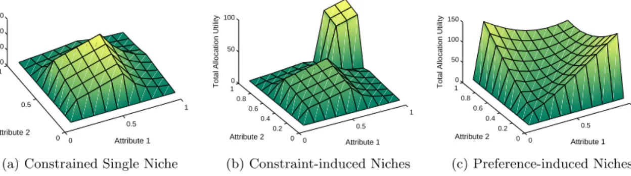
In terms of the trader context, in this paper we present results using three different contexts, examples of which are shown in Figure 1. Importantly, the trader contexts we use for these simulations cover situations where there are less market niches than there are market-exchanges ure 1a), as well as when there are multiple niches (Fig-ures 1b–1c). Each trader context contains a number of mar-ket niches and marmar-ket-exchanges’ ALS strategies must ex-plore the attribute-level space to find these. The landscapes in Figure 1 show, under ideal conditions, the maximum util-ity that could be generated if markets for the resource types described by thexandyaxes existed. Market-exchanges can be expected to generate revenue proportional to the height of the peaks. However, these landscapes are only ideal rep-resentations. In reality the height of these peaks can change throughout simulations as competing market-exchanges, as well as the trader population, learn. Further, the charging scheme used by the market-exchanges can have a significant impact on their ability to locate these niches and the amount of revenue each generates. More details on how these trader contexts are formed can be found in Chapter 5 of [13].
3.2.2
Charging contexts
The profit a market-exchange receives by offering a market for a certain resource type is influenced not only by that resources location in the attribute-level landscape, but also by the charging scheme used to generate that profit. As de-scribed in Section 2.3 it is assumed for these introductory investigations that market-exchange make use of three types of charges. We consider three charging contexts in this pa-per where each of the charges is used in isolation, so that we may see the impact it has on the exchanges ability to locate market niches.
The first charging context considered is the Registration Fee context. Market-exchanges using this context charge each trader that joins their exchange each day a fixed amount; for all simulations within this paper the registration fee ζmk
reg = 0.01. The second charging context considered is the
Transaction Price Feecontext. Market-exchanges using this context only charge traders when they successfully transact in the market. Specifically, each trader is charged a percent-age of the transaction price of the trade; for all simulations
within this paper, the percentage ζmk
tra = 0.01. The third charging context considered is the Bid/Ask Spread Com-mission context. Market-exchanges using this context only charge traders who successfully transact a portion of the
spread—the difference between their shout and the transac-tion price. Because this charging context only taxes traders on profit, they will never make a loss in a market using this charging context. For all simulations within this paper, the percentage chargedζmk
com= 0.01.
4.
AGENT-BASED SIMULATION STUDY
In this section we carry out a significant computational study of the market-based system described so far in this paper, and specifically on the applicability and performance of attribute-level selection strategies with respect to tackling the auto-matic co-niching problemin bilateral simulations of compet-ing market-exchanges. Firstly, we briefly describe the gen-eral setup used throughout. Every simulation last for 5000 trading days, and the mean values from 50 repetitions of each simulation variant are reported. The trading popula-tion used in each simulapopula-tion comprises 300 trader and is composed of an equal number of buyers and sellers; depend-ing on the trader context bedepend-ing used the constraints and preferences of the traders may differ. For each simulation repetition, along with a newrandom seed, all traders’ bud-get constraints were randomly generated according to the normal DistributionN(6,0.7) creating new supply and de-mand schedules each time.
Due to the complex nature of interactions between these economic agents it is unwise to assume that data samples will be normally distributed. To overcome this assumption rigorous statistical analysis is carried out. To test for nor-mality, all data samples are subjected to theLilliefors Test, a goodness of fit test for the Normal distribution. If samples are found to be non-normally distributed then they are com-pared using the non-parametricWilcoxon Signed-rank Test, otherwise apaired sample T-Test is used.
4.1
Experimental Results
The empirical analysis is carried out in two main parts. In the first part we consider competition between two market-exchanges over a single market niche. Many simulation vari-ations are carried out, using different combinvari-ations of charg-ing and trader context, in order to ascertain the ability of various ALS strategies for finding and holding onto a market niche. In the second part of the study we consider competi-tion between two market-exchanges in environments where there are multiple market niches. Again many combinations of environmental contexts are considered, however the em-phasis is on theco-niching ability of the market-exchanges, and what impact contexts have on the allocative efficiency of the entire system.
4.1.1
Competition over single market niches
In this set of simulations we consider theConstrained Single Nichetrader context, as shown in Figure 1a. Specifically, for this trader context we run simulations of all environmen-tal contexts formed from all combinations of the charging contexts and competitor pairings; this results in 90 environ-mental contexts and some 90×50 = 4500 simulations (each simulation variant is repeated 50 times).
Performance of ALS strategies is measured quantitatively by looking at the profit that each market-exchange makes
0 0.5 1 0 0.5 1 0 20 40 60 Attribute 1 Attribute 2
Total Allocation Utility
(a) Constrained Single Niche
0 0.5 1 0 0.2 0.4 0.6 0.8 1 0 50 100 Attribute 1 Attribute 2
Total Allocation Utility
(b) Constraint-induced Niches 0 0.5 1 0 0.2 0.4 0.6 0.8 1 0 50 100 150 Attribute 1 Attribute 2
Total Allocation Utility
(c) Preference-induced Niches
Figure 1:Three differenttrader contexts. (a) TheConstrained Single Nichecontext only has one population of traders interested in the
same niche. Buyers have maximum constraints on both attributes, which creates a market niche at the point for resourceπ=h0.6,0.6i.
(b) TheConstraint-induced Nichestrader context comprises two trader sub-populations and two market niches. One population prefers
to trade resources with high-level attributes—the most desirable types being at the market niche for resourceπ=h1.0,1.0i. The other
population, due to maximum constraints, most desires to trade resourcesπ=h0.6,0.6i. (c) ThePreference-induced Nichestrader context
also comprised two trader sub-populations and two market-niches. Unlike theConstraint-induced trader context the niches within this
context are formed from the preferences traders have over resource attributes. One subpopulation prefers to trade resourcesπ=h1.0,0.2i,
while the other subpopulation prefers to trade resourcesπ=h0.2,1.0i.
-dec -gre EA 1+1 ES Rank-based Softmax
-dec 2.477 3.585 3.157 3.527 1.878 0.70 (0.01) 1.329 1.120 1.096 1.310 0.206 (0.83) 0.302 0.259 0.309 0.303 -gre 1.720 3.449 3.111 3.256 1.529 0.916(0.01) 1.361 1.029 1.125 1.372 0.205 (0.82) 0.255 0.220 0.283 0.273 EA 0.292 0.252 0.449 0.642 0.053 0.232 0.201 0.523 (0.07) 0.421 0.625 0.056 0.049 0.060 (0.02) 0.099 0.101 1+1 ES 1.027 0.831 2.358 1.932(0.2) 0.645 0.461 0.543 0.753 (0.07) 0.764 0.962 0.090 0.098 0.107 (0.04) 0.089 (0.90) 0.128 Rank 0.444 0.435 1.239 1.365 (0.2) 1.326 0.496 0.496 1.006 0.668 (0.36) 1.089 0.151 0.141 0.146 0.094 (0.90) 0.124 Softmax 2.586 (0.02) 2.722 3.634 3.442 0.637 0.260 0.197 0.438 0.287 0.345 0.036 0.025 0.079 (0.07) 0.042 0.084
Table 1: Meansimulation profit for market-exchanges involved in bilateral simulation using various ALS strategies in environments
containing theConstrained Single Nichetrader context. Each profit value belongs to a market-exchange using the ALS strategy on that
row, in competition with an exchange using the ALS strategy in thatcolumn. Each cell has three profit values, representing simulations
where one of the charging contexts was in use: (top)Transaction Price Fee charging context; (middle)Registration Fee context; and
(bottom)Bid/Ask Commission context. Thus, the value in the absolute top-right of the table (1.878) represents-decreasing’s mean
profit in simulations againstSoftmax, when theTransaction Price Fee charging context was in use. Emboldened values indicate the
result is greater than the competitor’s and the samples are statistically distinct. Allp-valuesless than 0.005 are omitted, otherwise they
are shown to the right of profit values.
over the life of simulation, when using each of the ALS strategies to choose the resource types to be traded within its market. Self-play simulations, where both exchanges use the same strategy are not considered, because results in ex-pectation would be identical in these cases.
All results for this set of experiments are shown in Ta-ble 1. In general the reader will note that the emboldened profit values towards the top of the table indicate that the two semi-uniform bandit strategies located there, -greedy
and -decreasing, performed the strongest out of the ALS strategies in almost all of the environmental contexts. How-ever, it is clear that there are some strong performances by other ALS strategies incertain circumstances. For example, when theTransaction Feecharging context was in place (top cell row) theSoftmax ALS strategy (bottom row of table) performed statistically better than-greedyand others. This
suggests thatSoftmax is particularly sensitive to the charg-ing context in use, but that its proportional exploration may be better than-greedy’s under ideal conditions. Finally, it is clear that the evolutionary optimisation approaches do not perform as well as the bandit algorithms. This is a particu-larly interesting result, and closer examination of data traces from individual simulations reveals that in single niche en-vironments, the competing market-exchange is able to ‘flat-ten’ the profit landscape by attracting all of the traders to its exchange. In such a situation the 1+1 ES and EAALS strategies are unable to navigate the attribute-level land-scape because all points return no fitness (due to no traders joining their exchange). While they can attract traders back, often they are unable to due to being in poor parts of the attribute-level landscape, and relying on moving to neigh-bouring points to make progress.
4.1.2
Market co-niching in multi-niche environments
In this set of simulations, rather than looking directly at the profitability of the ALS strategies, we look at the niching be-haviour of the strategies, and the overall allocative efficiency of system. Of particular interest is whether two market-exchanges, in competition with each other, are able to locate and satisfy multiple market niches, leading to efficient and stable allocations. For this set of experiments we consider the two multi-niche trader contexts:Constraint-induced Niches
and Preference-induced Niches, as shown in Figure 1b–1c. Again, all bilateral combinations of ALS strategies were run within the two trader contexts, and each variant repeated for different charging contexts. Further, self-play simulations were considered as in a multi-niche environment how a strat-egy interacts—either competitively or cooperatively—is im-portant.
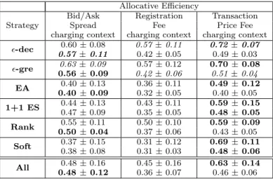
Allocative efficiency results are shown in Table 2 for all simulation variations. The allocative efficiency metric mea-sures directly the amount of utility (social welfare) gener-ated in the system each trading day and compares it to the theoretical maximum, which is calculated using a bespoke optimisation algorithm (see Chapter 4 [13]). In reality it is not possible for the efficiency to be continually close to 1.0, because of the complex nature of the system.
We find from our simulations that in general no charging context leads to the most efficient allocations across all possi-ble environmental contexts. In general we note that while the
Transaction Price Fee charging context is generally better for environments with the Constraint-induced trader con-text, the Bid/Ask Commission charging context is prefer-able when thePreference-induced trader context is present. TheRegistration Fee charging context is never preferable is one wishes to maximiser efficiency. This is most likely be-cause market-exchanges have little incentive to locate niches precisely as all points within the general location of a niche will result in about the same number of traders joining the exchange (and thus similar revenues). Finally, we again note that the presence of either of the two semi-uniform bandit strategies tends to result in the higher allocative efficiencies seen.
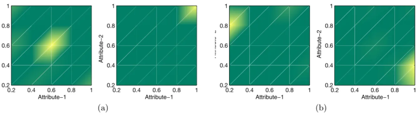
For the final analysis of the multi-niche environments we provide the reader with visualisations that allow one to get an understanding of the typical niching behaviour for various environment contexts. In Figure 2 we provide visualisations of two typical simulations. The first simulation, Figure 2a, is taken from a simulation where the Constraint-induced
trader context was used, and where the Transaction Price Fee charging context was in place. Two market-exchanges (each using theSoftmax ALS strategy) are competing over two market niches, and as one can see from the the visuali-sation, they both settle on separate niches, leading to a very efficient allocative efficiency (∼78%) and a profitable out-come for both. TheTransaction Price Fee charging context allows the ALSs to accurate locate the market niches.
In the second simulation, Figure 2b, we show a situation where thePreference-induced trader context is in place, and the Bid/Ask Commission charging context is used by the exchanges, which are both using-greedy ALS strategy. In this case the market-exchanges get quite close to the niches, but don’t precisely satisfy them (allocative efficiency was
∼64%). Interestingly, this may be due to market-exchanges generating more revenue from less efficient markets with this charging context; thus by staying slightly away from the
Allocative Efficiency Strategy
Bid/Ask Registration Transaction
Spread Fee Price Fee
charging context charging context charging context
-dec 0.570.60±±0.080.11 0.570.42±±0.110.05 0.720.49±±0.070.03 -gre 0.63±0.09 0.57±0.12 0.70±0.08 0.56±0.09 0.42±0.06 0.51±0.04 EA 0.40±0.13 0.36±0.11 0.49±0.12 0.40±0.09 0.32±0.05 0.40±0.05 1+1 ES 0.440.47±±0.130.09 0.350.43±±0.110.05 0.480.59±±0.150.05 Rank 0.55±0.11 0.50±0.10 0.59±0.09 0.50±0.04 0.37±0.06 0.43±0.05 Soft 0.37±0.15 0.31±0.12 0.69±0.11 0.38±0.08 0.31±0.03 0.48±0.06 All 0.48±0.16 0.45±0.16 0.63±0.14 0.48±0.12 0.36±0.07 0.46±0.06 Table 2: For each strategy, each data point provides the
mea-sure of system-wide mean daily allocative efficiency, overall
sim-ulations involving each strategy and its competitors (including against itself). Thus, it captures the impact that the presence of that strategy typically has on resource allocations within the sys-tem. Results are separated into the three different charging con-texts, thus each value is the mean from a sample of data points
with size: 6 competitor variations×50 simulation repetitions. A
value of 1.0 would indicate a 100% efficient allocation for every day of every reported simulation—a very unlikely outcome given the complex and dynamic nature of the system. Results are fur-ther separated according to the trader context in use. The top
value in each cell refers to the Constraint-induced trader
con-text, while the bottom value in each cell refers to the
Preference-inducedtrader context. For each ALS strategy and trader context,
emboldened values indicate highest reported efficiency across the three charging contexts. Emphasised values indicate the highest
reported efficiency for any strategy involved within that single
charging and trader context.
optimal market niche point, a wider spread and a larger commission can be maintained.
5.
CONCLUSIONS
This paper has presented a novel model for allocating multi-attribute resources via competing marketplaces. Traders choose to trade in the markets for resources that most satisfy their preferences and constraints, while marketplaces choose what type of resource should be traded within their markets. This model of resource allocation is novel because it is the first to explicitly consider the allocation of multi-attribute resources via multiple double auction marketplaces. Developing such a model required developing several new behaviour models and algorithms not considered within the literature. This paper provided the first formulation of the automatic co-niching problem, whereby market-exchanges must autonomously search the attribute-level space in search of resource-types that lie onmarket niches.
The main contribution of this paper is to provide the first computational study of several reinforcement learning ap-proaches to tackling the automatic co-niching problem, in the form of ALS strategies. The study was carried out by running over 10,000 bilateral market-based simulations com-prising hundreds of traders with differing preferences and constraints. In general we found that all ALS strategies are sensitive to at least some environmental factors, and thus none can be seen to generalise across all contexts, but in
0.2 0.4 0.6 0.8 1 0.2 0.4 0.6 0.8 1 Market−Exchange 1 Attribute−1 Attribute −2 0.2 0.4 0.6 0.8 1 0.2 0.4 0.6 0.8 1 Market−Exchange 2 Attribute−1 Attribute −2 (a) 0.2 0.4 0.6 0.8 1 0.2 0.4 0.6 0.8 1 Market−Exchange 1 Attribute−1 Attribute −2 0.2 0.4 0.6 0.8 1 0.2 0.4 0.6 0.8 1 Market−Exchange 2 Attribute−1 Attribute −2 (b)
Figure 2:Heat Maps showing typical niching behaviour of several attribute-level strategies. The maps aggregate the decisions of the ALS strategies over many thousands of trading days. Lighter areas indicate that the point in the attribute-level space was chosen more
frequently. (a) Typical performance of two market-exchanges each using aSoftmax ALS in theTransaction Price Fee charging and
Constraint-induced trader contexts. Two niches exist:π=h0.6,0.6iandπ=h1.0,1.0i(see Figure 1b). (b) Typical performance of two
-greedyALS strategies in thePreference-induced trader context along with theBid/Ask Spread Commissioncharging context. The two
niches are located atπ=h0.2,1.0iandπ=h1.0,0.2i(see Figure 1c).
most environmental contexts, at least one of the strategies performs very well.
In particular we have shown that it is possible for market-exchanges to autonomously locate market niches within these types of environments. We have also identified that strate-gies that rely on quantitative reward values, e.g.,Softmax
can be brittle and sensitive to parametric settings in these environments, while strategies that only rely on qualitative comparisons of rewards from actions, e.g.,-greedy and -decreasing are more robust. Further, we note that evolu-tionary approaches to attribute-level selection were not as successful as bandit approaches. While we believe this is down to the manipulating of the fitness landscape by com-petitors, a more detailed investigation into this phenomena, as well as improving the robustness of parametrically sensi-tive strategies will form some of our future work.
6.
REFERENCES
[1] Bichler, M., and Kalagnanam, J.Configurable offers and winner determination in multi-attribute auctions.European Journal of Operational Research 160, 2 (2005), 380–394.
[2] Broberg, J., Venugopal, S., and Buyya, R.
Market-oriented grids and utility computing: The state-of-the-art and future directions.Journal of Grid Computing 6, 3 (2008), 255–276.
[3] Cai, K., Niu, J., and Parsons, S.On the economic effects of competition between double auction markets. In10th Workshop on Agent-Mediated Electronic Commerce (AMEC 2008).(Estoril, Portugal, 2008). [4] Clearwater, S. H.Market-based control: a paradigm
for distributed resource allocation. World Scientific, Singapore, 1996.
[5] Cliff, D., and Bruten, J.Zero is Not Enough: On The Lower Limit of Agent Intelligence For Continuous Double Auction Markets. Tech. Rep. HPL 97-141, HP Laboratories Bristol, 1997.
[6] Gerding, E., McBurney, P., and Yao, X.
Market-based control of computational systems: introduction to the special issue.Autonomous Agents and Multi-Agent Systems. Special Issue on
Market-Based Control of Complex Computational
Systems. 21, 2 (2010), 109–114.
[7] Keeney, R. L., and Raiffa, H.Decisions with Multiple Objectives: Preferences and Value Tradeoffs. John Wiley & Sons, NY, USA, 1976.
[8] Lilien, G. L., Kotler, P., and Moorthy, K. S.
Marketing Models. Prentice-Hall, 1992. [9] Niu, J., Cai, K., Parsons, S., Gerding, E.,
McBurney, P., Moyaux, T., Phelps, S., and Shield, D.JCAT: a platform for the tac market design competition. In7th International joint conference on Autonomous agents and multiagent systems: (AAMAS ’08) (2008), pp. 1649–1650. [10] Robbins, H.Some aspects of the sequential design of
experiments.Bulletin of the American Mathematical Society 58, 5 (1952), 527–535.
[11] Roberts, J. H., and Lilien, G. L.Explanatory and predictive models of consumer behavior. InHandbooks in Operations Research and Management
Science:Volume 5: Marketing, J. Eliashberg and G. L. Lilien, Eds. North-Holland, 1993, pp. 27–82.
[12] Robinson, E., McBurney, P., and Yao, X.How specialised are specialists? generalisation properties of entries from the 2008 and 2009 TAC market design competitions. InAgent-Mediated Electronic Commerce: Designing Trading Strategies and Mechanisms, E. D. et al., Ed., vol. 59 ofLNBIP. Springer, 2010, pp. 178–194.
[13] Robinson, E. R.Resource Allocation via Competing Marketplaces. Ph.D. dissertation available:
http://bit.ly/kumsfc, Department of Computer Science, University of Birmingham, 2011.
[14] Sutton, R., and Barto, A.Reinforcement learning: An introduction. The MIT press, 1998.
[15] Whittle, P.Restless bandits: Activity allocation in a changing world.Journal of applied probability (1988), 287–298.