Neural coding with deep learning

(1)

PDF hosted at the Radboud Repository of the Radboud University

Nijmegen

The following full text is a publisher's version.

For additional information about this publication click this link.

http://hdl.handle.net/2066/191805

Please be advised that this information was generated on 2019-06-01 and may be subject to

change.

(2)

Neural coding

with deep learning

Umut GÜÇLÜ

NEURAL

CODING WITH DEEP

LEARNING

(3)

Neural coding

with

deep learning

(4)

ISBN

978-94-6284-147-5

Cover

Robert Voight

(5)

Neural coding

with

deep learning

Proefschrift

ter verkrijging van de graad van doctor

aan de Radboud Universiteit Nijmegen

op gezag van de rector magnificus

prof. dr. J.H.J.M. van Krieken,

volgens besluit van het college van decanen

in het openbaar te verdedigen op

donderdag 7 juni 2018 om

13:00 uur precies door

Umut Güçlü

geboren op

25 april 1986 te

Ankara (Turkije)

(6)

Promotoren

Prof. dr. ir. P.W.M. Desain

Prof. dr. D.G. Norris

Copromotor

Prof. dr. M.A.J. van Gerven

Manuscriptcommissie

Prof. dr. R.J.A. van Wezel

Prof. dr. P.R. Roelfsema (VU)

Dr. H.S. Scholte (UvA)

(7)

Neural coding

with

deep learning

Doctoral thesis

to obtain the degree of doctor

from Radboud University Nijmegen

on the authority of the Rector Magnificus

prof. dr. J.H.J.M. van Krieken,

according to the decision of the Council of Deans

to be defended in public on

Thursday, June 7, 2018 at

13:00 hours by

Umut Güçlü

Born on

April 25, 1986 in

Ankara (Turkey)

(8)

Supervisors

Prof. dr. ir. P.W.M. Desain

Prof. dr. D.G. Norris

Cosupervisor

Prof. dr. M.A.J. van Gerven

Doctoral Thesis Committee

Prof. dr. R.J.A. van Wezel

Prof. dr. P.R. Roelfsema (VU Amsterdam)

Dr. H.S. Scholte (University of Amsterdam)

(9)

„

The neurochemistry of the brain is astonishingly busy, the circuitry of a machine more wonderful than any devised by humans. But there is no evidence that its functioning is due to

anything more than the 1014_neural

connections that build an elegant architecture of consciousness.

—Carl Edward Sagan

(10)

(11)

1.1 Introduction

A fundamental question in neuroscience is how the human brain makes sense of its environment. How does the brain manage to learn about, represent and recognize statistical invariances in the environment that guide its actions, ultimately ensuring our survival in a world that is in a continuous state of flux? The representation of invariant features of the environment is the subject matter of sensory neuroscience. In recent years, artificial neural networks have become a popular vehicle for probing how brains respond to their surroundings.

Artificial neural networks are computational models that consist of idealized artificial neurons and aim to mimic crucial aspects of information processing in biological neural networks. In engin-eering, they have been shown to be highly effective in complex problem-solving.

Artificial neural networks were initially conceived of as an ap-proach to model mental or behavioral phenomena. This field is also referred to asconnectionism(Hebb, 2002) and was pop-ularized in the 1980’s under the nameparallel distributed

pro-cessing (McClelland & Rumelhart, 1989). Artificial neural

net-works were inspired by their biological counterparts (Fukushima, 1980) but have since become tools that are mostly used by engin-eers. Interestingly, cognitive neuroscientists are now rediscovering the use of artificial neural networks in furthering our understand-ing of neural information processunderstand-ing in the human brain.

In this chapter, we review how artificial neural networks can be used to probe human brain function with a focus on the state-of-the-art results that emerged from this approach. We proceed as follows. First, we describe how one can model the mapping between stimuli and responses in the human brain through the development of encoding models. Next, we focus on how the

(15)

mapping from static naturalistic stimuli to neural responses can be realized using artificial neural networks. Then we move on to describing how brain responses induced by dynamically changing naturalistic environments can be modeled. We end this chapter by outlining the rest of this thesis.

Modeling brain responses

We are interested in modeling how brains respond to their nat-ural environment. That is, the goal is to model how complex and semantically rich naturalistic stimuli influence neural re-sponses (Creutzfeldt & Nothdurft, 1978; Felsen & Dan, 2005). This objective can be achieved through the development of an

en-coding modelwhich seeks to explain (1) how a stimulus modulates

the activity of multiple neuronal populations and (2) how popula-tion activity affects data recorded at the sensor level (Kriegeskorte, 2015; Naselaris, Kay, Nishimoto & Gallant, 2011).

Consider an experiment in whichn(high-dimensional) stimulixt

are presented to a subject at timestiwithi= 1, . . . , N. We use

theN×Kmatrix

X= [xt1, . . . ,xtN]

> _(1.1)

to denote all N stimuli of dimensionK. For instance, X may be the sequence of all (vectorized) images that were shown in a vision experiment.

We are interested in the question how the external environment drives the responses of multiple neuronal populations to the stim-uliX. To this end, we introduce the notion of afeature space:

(16)

φ(xt) = (φ1(xt), . . . , φP(xt))> (1.2)

which captures sensory transformations.

During the experimental run, measurement vectorsyare obtained acrossQsensors, reflecting the responses induced by the presen-ted stimuli. For example, in functional magnetic resonance ima-ging (fMRI),yiis the blood oxygenation level-dependent (BOLD)

response for voxeliwhereas in MEG it reflects the magnetic field generated by the (weighted) activity of multiple pools of neurons. Throughout the experiment, these measurement vectors are col-lected at timesuj withj = 1, . . . , M, yielding theM×Qmatrix

of measurements

Y= [yu1, . . . ,yuM]

> _(1.3)

An encoding model makes explicit how population activity is measured at the sensor level. These measurements may depend on the history of population activity, e.g. due to the hemodynamic lag when collecting fMRI BOLD data.

To accommodate for these lagged responses, let

ψ_t(i)= (φi(xt−∆t), . . . , φi(xt))> (1.4)

denote the history of neural activity in the ith population for a given ∆t. Let ψt = vec(ψ

(1) t , . . . , ψ

(P)

t ). We now define the

(17)

b

yt=r(ψt) (1.5)

withr= (r1, . . . , rQ)>whererj is theforward modelwhich maps

(lagged) feature vectors to thejth sensor. Hence, development of an encoding modelr(ψt)requires making a choice about the used feature representation as well as the used forward models.

As we will see in upcoming sections, artificial neural networks are an ideal basis for encoding models that map external stimuli to observed brain responses. Here, alternative network architectures provide neuroscientists with the freedom to incorporate different modeling assumptions. We refer to encoding models that employ artificial neural networks asANN-based encoding models.

Artificial neural networks

Before outlining how artificial neural networks can be used to model stimulus-response relationships in neuroscience, we provide the reader with some theoretical background.

Artificial neural networks (ANNs) are inspired by biological neural networks in two respects (Haykin, 1994). First, knowledge is acquired by the network through a learning process. Second, in-terneuron connection strengths referred to as (synaptic) weights are used to store the knowledge. Artificial neural networks have been around for over seventy years (McCulloch & Pitts, 1943; Copeland & Proudfoot, 1996) but have fallen in and out of favor several times throughout the course of their history. In the follow-ing, we describe the key elements of which neural networks are composed.

(18)

Anartificial neural network(ANN) is a system of interconnected processing units (artificial neurons) which exchange messages between each other. An artificial neuron transforms a (vector-valued) inputx into a scalar outputy by computingy = f(a). Here, f is the neuron’s activation function and a is known as the input activation, representing the neural firing rate. This activation is usually taken to be an inner product of the form

a=wT_x_{, where}_w_{are adjustable parameters, also referred to as}

synapticweights(an additional bias term can be absorbed in the weights by ensuring that one of the inputs is a constant). Each weightwiquantifies the strength with which theith presynaptic

input is connected to its post-synaptic neuron. The weightsw

can be tuned based on experience to maximize a certain objective function, thereby making ANNs capable of learning.

An ANN is fully characterized by the properties of its artificial neurons, itsarchitecture(how its neurons are connected to one an-other), as well as the employedlearning algorithm. The employed learning algorithm comes in three flavors: supervised learning, where the goal is to predict an output when given an input

vec-tor,unsupervised learning, where the goal is to discover a good

internal representation of the input, andreinforcement learning, where the goal is to learn to select an action to maximize expected utility. For additional details, we refer to a number of excellent reviews (Schmidhuber, 2015; LeCun, Bengio & Hinton, 2015).

Linear neural networks

Consider again our objective of modeling a stimulus-response mapping of the form shown in the previous equation. Let us assume that each measurement can be expressed as an instantan-eous linear combination of input features (i.e.ψ(i)_t =xt). That is,

(19)

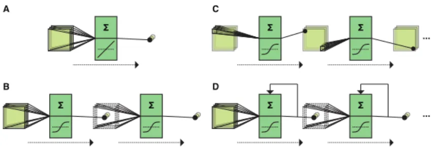
C

B A

D

Figure 1.1: Artificial neural network architectures.A: Linear neural net-work (multiple linear regression).B: Multi-layer perceptron consisting of one hidden layer and non-linear activation func-tions.C: Deep neural network with multiple convolutional hidden layers.D: Recurrent neural network where hidden states feed back onto themselves.

b

yt=(w>1xt, . . . ,w>Qxt)

> _(1.6)

=W>xt (1.7)

withW= [w1, . . . ,wQ]aP×Qmatrix of adjustable parameters.

It is easy to see that the previous equation implements alinear

neural networkwith inputsxt, outputsybt, weightsWand linear

activation functionf(a) =a(see Figure 1.1A).

Training of this encoding model amounts to estimating the para-metersW. In the neural network community, estimation of the parameters is cast as a gradient descent problem. Let

`(w) = 1 M M X t=1 ||_byt−yt||2 (1.8)

denote the squared loss function. Letw=vec(W) = (w1, . . . , wK).

(20)

∇`= ( ∂`

∂w1

, . . . , ∂`

∂wK

)> (1.9)

By using the iteration

w(n+1)←w(n)−(∇`)_w(n) (1.10)

withlearning rate, the weight vector converges to the optimal

weight vector (Widrow & Hoff, 1960).

Linear neural networks (i.e., multiple linear regression) can be used as an encoding model for modeling the stimulus-response transformation. Such an encoding model can be used to pre-dict stimulus-evoked responses directly. For example, they have previously been used for predicting human visual cortex voxel re-sponses (measured with fMRI) to handwritten characters (Schoen-makers, Barth, Heskes & van Gerven, 2013).

Multi-layer perceptrons

Multi-layer perceptrons(MLPs) are feed-forward neural networks

whose artificial neurons are organized in terms of layers (see Figure 1.1B). The classical MLP consists of one layer of input neurons, one layer of hidden neurons, and one layer of output neurons. It computes a non-linear function of the inputs:

(21)

where, in case of the classical MLP, we have

g=f2(W>₂f1(W>₁x)) (1.12)

where the elements offican be non-linear activation functions.

These properties extend the linear neural networks of the previous section. In fact, theuniversal approximation theoremtells us that MLPs consisting of one hidden layer can approximate any non-linear function with an arbitrary degree of precision given enough hidden neurons (Hornik, 1991; Cybenko, 1992).

In an MLP, minimization of a loss function also proceeds via a gradient descent procedure, as for the linear neural network case. However, due to the fact that the network consists of multiple layers, error derivatives need to be propagated backward from the output layer towards the input layer. It is this backpropagation algorithm which makes training of MLPs feasible (Rumelhart, Hinton & Williams, 1986).

Like linear neural networks, MLPs can also be used as an encoding model. For example, they have previously been used for predict-ing cat or monkey striate cortex neuron responses (measured with microelectrodes) to simple (e.g., bars) or compound (e.g., nat-ural images) stimuli (Lehky, Sejnowski & Desimone, 1992; Lau, Stanley & Dan, 2002; Prenger, Wu, David & Gallant, 2004). The encoding models that comprise a fixed nonlinear feature space and a linear forward model can also be seen as MLPs, whose first layer weights are fixed and second layer weights are learned. Some examples thereof are the use of Gabor wavelets (Marˆcelja, 1980) or semantic categories in combination with lasso or ridge regres-sion to predict human visual cortex voxel responses (measured with fMRI) to natural images or movies (Kay, Naselaris, Prenger

(22)

& Gallant, 2008; Naselaris, Prenger, Kay, Oliver & Gallant, 2009; Nishimoto et al., 2011a).

Deep neural networks

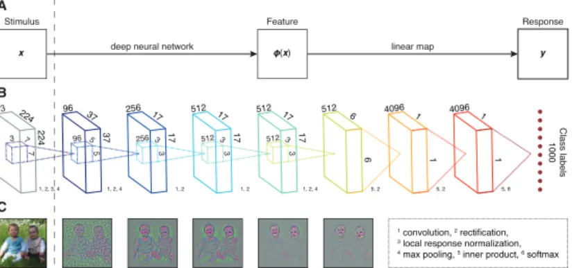
The classical MLP makes use of one hidden layer of artificial neurons. A recent trend is to train deep neural networks consisting of up to a thousand hidden layers (He, Zhang, Ren & Sun, 2015) (see Figure 1.1C).

Consider again the non-linear functiong. This function can also be written in terms of a composition of functions:

g(x) = (φL◦ · · · ◦φ1)(x) (1.13)

whereφlis the transformation given by the artificial neurons that

reside in thel-th layer of the neural network. In case the network contains more than one hidden layer, that is,L >2, we speak of

adeep neural network(DNN). Hence, DNNs are a special kind of

MLP whose artificial neurons are organized in terms of layers.

Deep neural networks entered the stage about thirty five years ago with Fukushima’s (1980) development of theNeocognitron. However, deep learning, i.e. backpropagation in deep neural networks has for a long time remained unfeasible, mainly due to instabilities in the weight updates. It was not until the start of the 21st century that deep learning gained traction. This can mainly be attributed to the curation of very large labeled datasets, the development of fast graphics processing units (GPUs), as well as the use of clever modifications to vanilla MLP training, such asrectified linear activation functions,dropout learningand

(23)

This breakthrough in training of deep neural networks led to a truly Cambrian explosion of research in deep learning, leading to quantum leaps in e.g. object recognition (Krizhevsky, Sutskever & Hinton, 2012), natural language processing (Sutskever, Vinyals & Le, 2014) and reinforcement learning (Mnih et al., 2015; Silver et al., 2016), often matching and sometimes surpassing human-level performance.

One might argue that DNNs are not particularly useful given the universal approximation property of MLPs that consist of one hid-den layer. However, it has been shown that many non-linear func-tions can be learned using much more compact deep architectures, compared to shallow architectures (Bengio, 2009). Moreover, the internal representations that emerge during DNN training have also been shown to be semantically meaningful (Zeiler & Fergus, 2013). That is, it was found that increasingly complex represent-ations are learnt by DNNs that are trained, e.g., to predict the category to which an input image belongs.

Deep neural networks can be used as a feature space for modeling the feature-response transformation. Such a feature space can be combined with any forward model to predict stimulus-evoked responses. Similarly, DNNs can be used as a feature space for rep-resentational similarity analysis (RSA) (Kriegeskorte, 2008). Such a feature space can be compared to stimulus-evoked responses directly.

In one of the first studies on this topic, Yamins et al. (2014) predicted monkey V4 and IT neuron responses (measured with microelectrodes) to natural images with a DNN after training it for object recognition. They showed that intermediate and top layers of the DNN were highly predictive of monkey V4 and IT neuron responses to natural images, respectively. These results have later been successfully reproduced in the monkey visual cortex, and similar results have then been reported in the human visual cor-tex (Agrawal, Stansbury, Malik & Gallant, 2014; Khaligh-Razavi

(24)

& Kriegeskorte, 2014; Cadieu et al., 2014). Khaligh-Razavi and Kriegeskorte (2014) also compared (with RSA) the visual recog-nition performance of 37 different models including DNNs (Kr-izhevsky et al., 2012), Gabor wavelets (Marˆcelja, 1980), GIST (Oliva & Torralba, 2001), HMAX (Poggio & Riesenhuber, 1999) and Vis-Net (Rolls & Milward, 2000) with one another as well as compar-ing the similarity of their representations to human and monkey IT representations (measured with fMRI). They showed that DNNs have not only the best visual recognition performance but also the most similar representations.

In Chapters 3-5, we extended these ideas to different tasks and areas. In Chapter 3, we probed human ventral stream represent-ations (measured with fMRI) with a two-dimensional (spatial) DNN after it has been pretrained for object recognition (in pho-tographs). In Chapter 4, we probed human dorsal stream repres-entations (measured with fMRI) with a three-dimensional (spati-otemporal) convolutional neural networks after finetuning it for action recognition (in movies). In Chapter5, we moved beyond the visual cortex and to the auditory cortex. That is, we probed human superior temporal gyrus representations (measured with fMRI) with one-dimensional (spectral and/or temporal) convolutional neural networks after training them for music recognition (e.g., genre, instrument, mood, etc.). These studies showed the exist-ence of a representational gradient such that increasingly deeper DNN layers better correspond to increasingly downstream areas in the human ventral stream, dorsal stream, and superior tem-poral gyrus as well as showing that this correspondence is driven by task-optimization and not exact architectural assumptions, which has been successfully reproduced since then (Seibert et al., 2016; Eickenberg, Gramfort, Varoquaux & Thirion, 2017). Simil-arly, Cichy, Khosla, Pantazis, Torralba and Oliva (2016), Seeliger et al. (2017) showed that the object recognition-optimized DNN-human ventral stream correspondence holds not only for space but also for time such that increasingly deep DNN layers better predict increasingly late stimulus-evoked human ventral stream

(25)

sensor or source responses (measured with MEG). Also, Kell, Yam-ins, Norman-Haignere and McDermott (2016) showed that the task-optimized DNN-human superior temporal cortex correspond-ence holds not only for music recognition- but also for speech recognition-optimized DNNs.

It is important to note that DNNs can also be used for classify-ing (Haxby, 2001; Kamitani & Tong, 2005), identifyclassify-ing (Kay et al., 2008; Mitchell et al., 2008) or reconstructing (Thirion et al., 2006; Miyawaki et al., 2008) a stimulus from voxel responses (meas-ured with fMRI) in the human brain. They have previously been used for reconstructing perceived handwritten characters (van Gerven, de Lange & Heskes, 2010). In Chapters 3-4, we used them for identifying perceived natural images. They have more recently been used for classifying perceived and imagined nat-ural images (Horikawa & Kamitani, 2017), and reconstructing perceived faces (Güçlütürk et al., 2017).

Word embedding

Deep neural networks can be used to represent increasingly ab-stract stimulus features. Arguably, at the top of this hierarchy one may encounter conceptual representations. Such representations can also be captured more directly by focusing on linguistic input. We will now consider a special kind of MLP for learning word embeddings. Such word embeddings can be used to probe directly where conceptual knowledge is represented in the human brain.

When using linguistic stimuli (e.g. words), a neural network needs to be able to use individual words as input. One way to achieve this is by assuming that, given a vocabulary of N words, the

nth word is encoded as a one-hot vector of lengthN, consisting of all zeros except for a one at thenth index. A problem with this approach is that the number of words in a vocabulary can

(26)

run in the hundreds of thousands, making use of this sparse representation prohibitive in practice.

An alternative approach is to use aword embeddingwhere each word is represented as a low-dimensional dense vector, providing

adistributed representationfor that word. The learning problem

is to map the sparse high-dimensional representation to a dense low-dimensional representation (Bengio, Ducharme, Vincent & Janvin, 2003).

This learning problem can be cast in terms of an MLP. Given a se-quence of wordsw1, w2, . . . , wT that together make up a text, the

skip-gram modelmaximizes the following objective function

(Miko-lov, Chen, Corrado & Dean, 2013b):

J = 1 T T X t=1 c X j=−c logp(wt+j |wt) (1.14)

Hence, the aim is to predict the context (surrounding) words given a target word.

This probability can be modeled using a neural network with one hidden layer (i.e. an MLP). The input-to-hidden weights are given byUand the hidden-to-output weights are given byV. The probability of a context wordw0 given a target word wis then expressed as p(w0|w) = exp(v > w0uw) PW i=1exp(v>wiuw) (1.15)

(27)

whereuwandvware the input and output vectors associated with

word wandW is the number of words in the vocabulary. The corresponding neural network uses a linear activation function for the hidden units and a softmax activation function for the output units. Lete(w)be the one-hot encoding of a word (e.g.

[0,0,0,1,0,0, . . . ,0,0]). Then, the word embedding ofwis given by vec(w)≡e(w)T_U₌_u

w=h.

Interestingly, the distributed representation of a word vec(w)

provides a semantically meaningful representation, even allow-ing for arithmetic expressions such as vec(king)−vec(man) +

vec(woman)≈vec(queen)(Mikolov, Yih & Zweig, 2013c).

The question of how the human brain encodes semantics has been extensively studied by mapping manually- or automatically-derived corpus representations to stimulus-evoked voxel responses (measured with fMRI) (Mitchell et al., 2008; Murphy, Talukdar & Mitchell, 2012; Huth, Nishimoto, Vu & Gallant, 2012; Fyshe, Murphy, Talukdar & Mitchell, 2013). Recent word embeddings such as W2V (Mikolov, Sutskever, Chen, Corrado & Dean, 2013a) and GloVe (Pennington, Socher & Manning, 2014) have been very successful in computational linguistics. They project words to continuous, distributed, low-dimensional vector space, where meanings of words, similarities between words and analogies are preserved.

Like DNNs, word embeddings can also be used as a feature space. Previously, Nishida, Gallant and Nishimoto (2015), Güçlü and van Gerven (2015) used word embeddings to predict downstream human visual cortex voxel responses (measured with fMRI) to semantic contents of natural images and movies. In Chapter 6, we used word embeddings while comparing different forward models. These studies showed that the human brain might be encoding semantics in a continuous, distributed, low-dimensional vector space, where many linguistic regularities are preserved. These results are reminiscent of the direct, predictive relationship

(28)

that was shown to exist between word co-occurrences and human brain activity (Mitchell et al., 2008).

Unsupervised learning

So far, we have focused on models that were trained in a super-vised manner. Another class of neural networks models is formed by those that are trained in an unsupervised manner on input data

D={x1, . . . ,xN}. Examples thereof are Hopfield networks

(Hop-field, 1982), Boltzmann machines (Ackley, Hinton & Sejnowski, 1985) and deep belief networks (Hinton, Osindero & Teh, 2006). Rather than minimizing a loss function that measures the differ-ence between observed and predicted output, these models aim to maximize the log probability of the input data, again using gradient descent procedures. That is, the update steps during gradient descent are given by

∆θ=−∂

P

nlogp(xn)

∂θ (1.16)

whereθis a model parameter.

Like supervised DNNs or word embeddings, unsupervised ANN variants can also be used as a feature space. Previously, van Ger-ven et al. (2010) used deep belief networks (Hinton et al., 2006) for reconstructing handwritten digits from stimulus-evoked voxel responses. Similarly, Güçlü and van Gerven (2013) used independ-ent componindepend-ent analysis (Hyvärinen & Oja, 2000) for predicting voxel responses to handwritten digits and reconstructing them from stimulus-evoked voxel responses. In Chapter 2, we used sparse coding for predicting voxel responses to natural images and identifying them from stimulus-evoked voxel responses. All of these studies were concerned with early visual areas of the human

(29)

brain (whose responses were measured with fMRI) and showed that unsupervised ANN variants could account for low-level neural representations. Arguably, unsupervised learning offers a more biologically plausible explanation of neural representations in comparison to its supervised counterpart. However, unsuper-vised ANN variants have not been as successful in accounting for high-level neural representations (Khaligh-Razavi & Kriegeskorte, 2014).

Recurrent neural networks

The feed-forward neural networks that have been reviewed so far are missing a key ingredient that is crucial to brain function, namely recurrence. Feed-forward neural networks make a new prediction at every time point, ignoring any temporal dependen-cies that might otherwise modulate their responses. However, it is clear that the brain does not function this way. That is, when confronted with a stimulus at a certain time point, the brain does not ignore everything that it has processed up to that time point. Rather, it takes into account the stimulus history and its responses are modulated by temporal dependencies.

In contrast to feed-forward neural networks, recurrent neural

networks(RNNs) are implementations of dynamical systems that

explicitly take temporal dependencies into account (Jordan, 1997; Elman, 1990) (see Figure 1.1D). Consider a RNN where inputs, hidden states and outputs at timetare given byxt,htandyt,

respectively. Effectively, RNNs can be seen as infinitely deep neural networks with the difference that each layer receives its own external input and produces an external output. LetUdenote the input-to-hidden weights,Vthe hidden-to-hidden weights and

Wthe hidden-to-output weights. We usef(·)andg(·)to denote the element-wise application of an activation function to a vector-valued input. In an RNN, updating of the hidden layers is given by

(30)

ht=f(Uxt+Vht−1)and updating of the output units is given

byyt=g(Wht).

A popular learning algorithm for recurrent neural networks is backpropagation through time (BPTT) (Werbos, 1990). It general-izes backpropagation for feed-forward networks to the recurrent case. This is done by unrolling the network so all cycles between units are removed while forcing the weights at each time point to be identical. In RNNs, when minimizing the error using gradient descent, one iterates over time rather than independent training examples, as in standard backpropagation.

It has been found that training of vanilla RNNs can be hard due to vanishing or exploding gradients in the BPPT gradient up-dates (Bengio, Simard & Frasconi, 1994). One way to improve RNN training is by endowing them with a memory, so events in the past can more easily update present network states. One way to realize this is through the use oflong short-term memory

(LSTM) layers (Hochreiter & Schmidhuber, 1997). LSTMs use memory cells surrounded by multiplicative gate units to store read, write and reset information. These gates, instead of sending their activities as inputs to other neurons, set the weights on edges con-necting the rest of the neural net to the memory cell. LSTMs can be trained with backpropagation using somewhat more involved gradients.

Recurrent neural networks can be used as a forward model for modeling the feature-response transformation. Such a forward model can then be combined with any feature space to predict stimulus-evoked responses. Previously, Joukes, Hartmann and Krekelberg (2014) used RNNs to model the dynamics of the neur-ons in monkey MT (measured with microelectrodes) and showed that RNNs can reproduce properties of MT neurons in the mon-key brain such as velocity computation better than nonrecurrent neural networks can. In Chapter 6, we used RNNs to model the dynamics of voxels in the human visual cortex (measured with

(31)

fMRI) and showed than RNNs can reproduce properties of visual cortex voxels in the human brain such as hemodynamic response better than nonrecurrent neural networks can.

ANN-based encoding models

In summary, the way in which the ANN variants have been used in the literature and/or in this thesis can be grouped in the following three overlapping categories:

• Using linear neural networks (multiple linear regression) (Schoen-makers et al., 2013) or multi-layer perceptrons (Lehky et al., 1992; Lau et al., 2002; Prenger et al., 2004) for model-ing the stimulus-response transformation (as an encodmodel-ing model). Such an encoding model can be used to directly predict stimulus-evoked responses.

• Using deep neural networks (Yamins et al., 2014; Agrawal et al., 2014; Eickenberg et al., 2017), word embedding (Nishida et al., 2015; Güçlü & van Gerven, 2015) or unsupervised learning (van Gerven et al., 2010; Güçlü & van Gerven, 2013) for modeling the stimulus-feature transformation (as a feature space). Such a feature space can be combined with any forward model to indirectly predict stimulus-evoked responses. This is also the approach taken in Chapters 2-6.

• Using recurrent neural networks (Joukes et al., 2014) for modeling the feature-response transformation (as a for-ward model). Such a forfor-ward model can be combined with any feature space to indirectly predict stimulus-evoked re-sponses. This is also the approach taken in Chapter 6.

(32)

1.2 Outline

Chapter 2 In Chapter 2, to overcome the challenge of formalizing

what stimulus features should modulate single voxel responses, we introduce a general approach for making directly testable predictions of single voxel responses to statistically adapted rep-resentations of ecologically valid stimuli. These reprep-resentations are learned from unlabeled data without supervision. Our ap-proach is validated using a parsimonious computational model of (i) how early visual cortical representations are adapted to statistical regularities in natural images and (ii) how populations of these representations are pooled by single voxels. This compu-tational model is used to predict single voxel responses to natural images and identify natural images from stimulus-evoked mul-tiple voxel responses. We show that statistically adapted low-level sparse and invariant representations of natural images better span the space of early visual cortical representations and can be more effectively exploited in stimulus identification than hand-designed Gabor wavelets. Our results demonstrate the potential of our approach to better probe unknown cortical representations.

Chapter 3 In Chapter 3, we quantitatively show that there indeed

exists an explicit gradient for feature complexity in the ventral pathway of the human brain. This is achieved by mapping thou-sands of stimulus features of increasing complexity across the cortical sheet using a deep neural network. Our approach also re-veals a fine-grained functional specialization of downstream areas of the ventral stream. Furthermore, it allows decoding of repres-entations from human brain activity at an unsurpassed degree of accuracy, confirming the quality of the developed approach. Stimulus features that successfully explain neural responses indic-ate that population receptive fields are explicitly tuned for object categorization. This provides strong support for the hypothesis that object categorization is a guiding principle in the functional organization of the primate ventral stream.

(33)

Chapter 4 In Chapter 4, we explore whether deep neural net-works also provide accurate predictions of neural responses across the dorsal visual pathway, which is thought to be devoted to motion processing and action recognition. This is achieved by training deep neural networks to recognize actions in videos and subsequently using them to predict neural responses while sub-jects are watching natural movies. Moreover, we explore whether dorsal stream representations are shared between subjects. In order to address this question, we examine if individual subject predictions can be made in a common representational space estimated via hyperalignment. Results show that a deep neural network trained for action recognition can be used to accurately predict how dorsal stream responds to natural movies, revealing a correspondence in representations of deep neural network layers and dorsal stream areas. It is also demonstrated that models operating in a common representational space can generalize to responses of multiple or even unseen individual subjects to novel spatio-temporal stimuli in both encoding and decoding settings, suggesting that a common representational space underlies dorsal stream responses across multiple subjects.

Chapter 5 In Chapter 5, we develop task-optimized deep neural

networks that achieve state-of-the-art performance in different evaluation scenarios for automatic music tagging. These deep neural networks are subsequently used to probe the neural rep-resentations of music. Representational similarity analysis reveal the existence of a representational gradient across the superior temporal gyrus. Anterior superior temporal gyrus is shown to be more sensitive to low-level stimulus features encoded in shallow deep neural network layers whereas posterior STG is shown to be more sensitive to high-level stimulus features encoded in deep deep neural network layers.

Chapter 6 In Chapter 6, we investigate the extent to which

(34)

for nonlinear processing of arbitrary feature sequences to predict feature-evoked response sequences as measured by functional magnetic resonance imaging. We show that the proposed re-current neural network models can significantly outperform es-tablished response models by accurately estimating long-term dependencies that drive hemodynamic responses. The results open a new window into modeling the dynamics of brain activity in response to sensory stimuli.

(35)

(36)

(37)

2

Unsupervised feature

learning improves

prediction of human

brain activity in

response to natural

images

This chapter is based on Güçlü, U. and van Gerven, M. (2014).

Unsupervised feature learning improves prediction of

human brain activity in response to natural images. PLOS

Computational Biology, 10(8):e1003724. https://doi.org/10.1371/ journal.pcbi.1003724

(38)

2.1 Introduction

An important goal of contemporary cognitive neuroscience is to characterize the relationship between stimulus features and hu-man brain activity. This relationship can be studied from two distinct but complementary perspectives of encoding and decod-ing (Dayan & Abbott, 2005). The encoddecod-ing perspective is con-cerned with how certain aspects of the environment are stored in the brain and uses models that predict brain activity in response to certain stimulus features. Conversely, the decoding perspective uses models that predict specific stimulus features from stimulus-evoked brain activity and is concerned with how specific aspects of the environment are retrieved from the brain.

Stimulus-response relationships have been extensively studied in computational neuroscience to understand the information contained in individual or ensemble neuronal responses, based on different coding schemes (Brown, Kass & Mitra, 2004). The invasive nature of the measurement techniques of these stud-ies has restricted human subjects to particular patient popula-tions (Quiroga, Reddy, Kreiman, Koch & Fried, 2005; Pasley et al., 2012). However, with the advent of functional magnetic reson-ance imaging (fMRI), encoding and decoding in fMRI has made it possible to noninvasively characterize the relationship between stimulus features and human brain activity via localized changes in blood-oxygen-level dependent (BOLD) hemodynamic responses to sensory or cognitive stimulation (Naselaris et al., 2011).

Encoding models that predict single voxel responses to certain stimulus features typically comprise two main components. The first component is a (non)linear transformation from a stimulus space to a feature space. The second component is a (non)linear transformation from the feature space to a voxel space. Encoding models can be used to test alternative hypotheses about what a voxel represents since any encoding model embodies a specific

(39)

hypothesis about what stimulus features modulate the response of the voxel (Naselaris et al., 2011). Furthermore, encoding mod-els can be converted to decoding modmod-els that predict specific stimulus features from stimulus-evoked multiple voxel responses. In particular, decoding models can be used to determine the specific class from which the stimulus was drawn (i.e. classifica-tion) (Haxby, 2001; Kamitani & Tong, 2005), identify the correct stimulus from a set of novel stimuli (i.e. identification) (Kay et al., 2008; Mitchell et al., 2008) or create a literal picture of the stim-ulus (i.e. reconstruction) (Thirion et al., 2006; Miyawaki et al., 2008; Schoenmakers et al., 2013).

The conventional approach to encoding and decoding makes use of feature spaces that are typically hand-designed by theorists or experimentalists (Kay et al., 2008; Mitchell et al., 2008; Miyawaki et al., 2008; Naselaris et al., 2009; Nishimoto et al., 2011a; Vu et al., 2011; Kay, Winawer, Rokem, Mezer & Wandell, 2013b). However, this approach is prone to the influence of subjective biases and restricted to a priori hypotheses. As a result, it severely restricts the scope of alternative hypotheses that can be formulated about what a voxel represents. This restriction is evident by a paucity of models that adequately characterize extrastriate visual cortical voxels.

A recent trend in models of visual population codes has been the adoption of natural images for the characterization of voxels that respond to visual stimulation (Kay et al., 2008; Naselaris et al., 2009). The motivation behind this trend is that natural images admit multiple feature spaces such as low-level edges, mid-level edge junctions, high-level object parts and complete objects that can modulate single voxel responses (Naselaris et al., 2011). Im-plicit about this motivation is the assumption that the brain is adapted to the statistical regularities in the environment (Barlow, 2012) such as those in natural images (Olshausen & Field, 1996; Bell & Sejnowski, 1997). At the same time, recent developments in theoretical neuroscience and machine learning have shown

(40)

that normative and predictive models of natural image statistics learn statistically adapted representations of natural images. As a result, they predict statistically adapted visual cortical repres-entations, based on different coding principles. Some of these predictions have been shown to be similar to what is found in the primary visual cortex such as topographically organized simple and complex cell receptive fields (Hyvärinen, 2010).

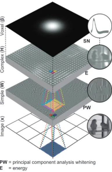
Building on previous studies of visual population codes and nat-ural image statistics, we introduce a general approach for making directly testable predictions of single voxel responses to statist-ically adapted representations of ecologstatist-ically valid stimuli. To validate our approach, we use a parsimonious computational model that comprises two main components (Figure 2.1). The first component is a nonlinear feature model that transforms raw stimuli to stimulus features. In particular, the feature model learns the transformation from unlabeled data without supervi-sion. The second component is a linear voxel model that trans-forms the stimulus features to voxel responses. We use an fMRI data set of voxel responses to natural images that were acquired from the early visual areas (i.e. V1, V2 and V3) of two sub-jects (i.e. S1 and S2) (Lescroart et al., 2011). We show that the encoding and decoding performance of this computational model is significantly better than that of a hand-designed Gabor wavelet pyramid (GWP) model of phase-invariant complex cells. The software that implements our approach is provided at http: //www.ccnlab.net/research/.

2.2 Materials and methods

Data

We used the fMRI data set (Lescroart et al., 2011) that was origin-ally published in (Kay et al., 2008; Naselaris et al., 2009). Briefly,

(41)

Voxel ( β ) Complex ( H ) Simple ( W ) Image ( x ) PW E SN PW E SN

= principal component analysis whitening = energy

= static nonlinearity

Figure 2.1: Encoding model. The encoding model predicts single voxel responses to images by nonlinearly transforming the im-ages to complex cell responses and linearly transforming the complex cell responses to the single voxel responses. For example, the encoding model predicts a voxel response to a 128×128 imagexas follows: Each of the 16 non-overlapping 32×32 patches of the image_bz(i)is first vectorized, prepro-cessed and linearly transformed to 625 simple cell responses, i.e.Wz(i)wherez(i)is a vectorized and preprocessed patch. Energies of the simple cells that are in each of the 625 partially overlapping 5×5 neighborhoods are then locally pooled, i.e. H(Wz(i)₎2_{, and nonlinearly transformed to}

one complex cell response, i.e. log(1 +H(Wz(i))2). Next, 10000 complex cell responses are linearly transformed to the voxel response, i.e. β>φ(x)where φ(x) = ((log(1 +

H(Wz(1))2)>, . . . ,(log(1 +H(Wz(16))2)>)>. The feature transformations are learned from unlabeled data. The voxel transformations are learned from feature-transformed stimulus-response pairs.

the data set contained 1750 and 120 stimulus-response pairs of two subjects (i.e. S1 and S2) in the estimation and validation sets, respectively. The stimulus-response pairs consisted of grayscale natural images of size 128×128 pixels and stimulus-evoked peak

(42)

BOLD hemodynamic responses of 5512 (S1) and 5275 (S2) voxels in the early visual areas (i.e. V1, V2 and V3). The details of the experimental procedures are presented in(Kay et al., 2008).

Problem statement

Encoding

Letx∈_Rd_and_y_∈

Rq be a stimulus-response pair wherexis a vector of pixels in a grayscale natural image, andyis a vector of voxel responses. Parametersdandqdenote the number of pixels that make up the image and voxels, respectively. Givenx, we are interested in the problem of predictingy:

b

y= arg max

y p(y|φ(x)) =B

>_φ₍_x₎ _(2.1)

where_byis the predicted response tox, andpis the encoding dis-tribution ofygivenφ(x). The functionφnonlinearly transforms

xfrom the stimulus space to the feature space, andBlinearly transformsφ(x)from the feature space to the voxel space.

Decoding

Let_Xbe a set of images that containsx. Given_Xandy, we are interested in the problem of identifyingx:

b

x= arg max

x∈Xρy,B

(43)

where x_b is the identified image from y, and ρ is the Pearson product-moment correlation coefficient betweenyandB>φ(x).

Solving the encoding and decoding problems requires the defin-ition and estimation of a feature modelφ followed by a voxel modelB.

Feature model

Model definition

Following Hyvärinen and Hoyer (2001), we summarize the defini-tion of the SC model. We start by defining a single-layer statistical generative model of whitened grayscale natural image patches. Assuming that a patch is generated by a linear superposition of latent variables that are non-Gaussian (in particular, sparse) and mutually independent, we first use independent component ana-lysis to define the model by a linear transformation of independent components of the patch:

Z=As (2.3)

wherez∈_Rn _{is a vector of pixels in the patch,}_A_∈

Rn×m_{is a}

mixing matrix, ands∈ _Rm_{is a vector of the components of}_z

such thatm≤n. The parametersnandmdenote the number of pixels and components, respectively. We then definesby inverting the linear system that is defined byA:

(44)

whereW∈ _Rm×n _{is an unmixing matrix such that}_W₌_A−1_.

We constrainWto be orthonormal andsito have unit variance

such thatsi are uncorrelated and unique, up to a multiplicative

sign. Next, we define the joint probability of sby the product of the marginal probabilities of si since si are assumed to be

independent: p(s) = m Y i=1 p(si) (2.5)

wherep(si)are peaked at zero and have high kurtosis sincesiare

assumed to be sparse.

While one of the assumptions of the model is thatsiare

independ-ent, their estimates are only maximally independent. As a result, residual dependencies remain between the estimates ofsi. We

continue by modeling the nonlinear correlations ofsisincesiare

constrained to be linearly uncorrelated. In particular, we assume that the locally pooled energies of si are sparse. Without loss

of generality, we first arrangesion a square grid graph that has

circular boundary conditions. We then define the locally pooled energies ofsiby the sum of the energies ofsithat are in the same

neighborhood:

c=Hs2 (2.6)

wherec∈_Rm_{is a vector of the locally pooled energies of}_s

i and

H∈_Rm×m_{is a neighborhood matrix such that}_h

i,j= 1ifcipools

the energy ofsjandhi,j= 0otherwise. Next, we redefinelogp(s)

(45)

logp(s)≈

m

X

i=1

G(ci) (2.7)

whereGis a convex function. Concretely, we useG(ci) =−log(1+ ci).

In a neural interpretation, simple and complex cell responses can be defined assand a static nonlinear function ofc, respectively. Concretely, we uselog(1 +c)to define the complex cell responses after we estimate the model.

Model estimation

We use a modified gradient ascent method to estimate the model by maximizing the log-likelihood ofW(equivalently, the sparse-ness ofc) given a set of patches:

c

W= arg max

W L(W|Z) (2.8)

whereL(W|Z) =−P

z(i)logp(H(Wz(i))2)is an approximation of the log-likelihood ofWandZ= (z(1),z(2), . . .)is the set of patches. At each iteration, we first find the gradient ofL(W|Z):

(46)

where◦is the Hadamard (element-wise) product. We then project it onto the tangent space of the constrained space (Edelman, Arias & Smith, 1998):

∇WL(W|Z) =∇WL(W|Z)−W∇WL(W|Z)>W (2.10)

Next, we use backtracking line search to choose a step size by reducing it geometrically with a rate from(0,1)until the Armijo-Goldstein condition holds (Boyd & Vandenberghe, 2004). Finally, we updateWand find its nearest orthogonal matrix:

W←W+µ∇WL(W|Z) (2.11)

W←(WW>)−12_W (2.12)

whereµis the step size.

Voxel model

Model definition

We start by defining a model for each voxel. Assuming that

p(y|φ(x)) ∼ N(B>φ(x),Σ), whereB = (β₁, . . . ,β_q) ∈ Rm×q

and Σ = diag(σ2

1, . . . , σ2q) ∈ Rq×q, we use linear regression to

define the models by a weighted sum ofφ(x):

(47)

whereεi∼ N(0, σi2).

Model estimation

We estimate the model using ridge regression:

b βi= arg min βi 1 N N X j=1 (y_i(j)−β_i>φ(x(j))) +λi||βi|| 2 2 (2.14) whereX= (x(1), . . . ,x(N))>_∈_RN×d_and_Y_{= (}_y(1)_{, . . . ,}_y(N)₎>_∈

RN×q _{is an estimation set, and}_λ

i≥0is a complexity parameter

that controls the amount of regularization. The parameter N

denotes the number of stimulus-response pairs in the estimation set. We obtainβbi as:

b βi = (λiIm+Φ>Φ)−1Φ>Yi (2.15) whereΦ= (φ(x(1)₎_{, . . . , φ}₍_x(N)₎₎>_∈ RN×m_and_Y i= (y(1)i , . . . , y (N) i )>∈ RN×1.

SincemN, we solve the problem in a rotated coordinate sys-tem in which only the firstNcoordinates ofΦare nonzero (Hastie, Tibshirani & Friedman, 2009; Murphy et al., 2012). We first fac-torizeΦusing the singular value decomposition:

(48)

whereUU> =U>U=IN,S=diag(s)∈RN×N andV>V =

IN. The columns ofU, the diagonal entries ofSand the columns

of V are the left-singular vectors, the singular values and the right-singular vectors ofΦ, respectively. We then reobtainβbias:

b

βi=Vdiag(

s s◦s+λi

)U>Yi (2.17)

where division is defined element-wise. The rotation reduces the complexity of the problem fromO(m3)toO(mN2). To choose the optimalλi, we perform hyperparameter optimization using grid

search guided by a generalized cross-validation approximation to leave-one-out cross-validation [60]. We define a grid by first sampling the effective degrees of freedom of the ridge regression fit from[1, N]since its parameter space is bounded from above. The effective degrees of freedom of the ridge regression fit is defined as: df(λi) = N X j=1 s2 j s2 j+λi (2.18)

We then use Newton’s method to solvedf forλi. Once the grid

is defined, we choose the optimal that minimizes the generalized cross-validation error: b λi= arg min λ∈Λ{ N X j=1 [y (j) i −yb (j) i (λ) 1−df(λ)/N] 2_} _(2.19)

(49)

Encoding and decoding

In the case of the SC model, each randomly sampled or non-overlapping patch was transformed to its principal components such that 625 components with the largest variance were retained and whitened prior to model estimation and validation. After the images were feature transformed, they were z-scored. The SC model of 625 simple and 625 complex cells was estimated from 50000 patches of size 32×32 pixels that were randomly sampled from the 1750 images of size 128×128 pixels in the estimation set. The details of the GWP model are presented in (Kay et al., 2008). The SC2 and GWP2 models were estimated from the 1750 feature-transformed stimulus-response pairs in the estimation set.

Voxel responses to an image of size 128×128 pixels were predicted as follows. In the case of the SC model, each 16 non-overlapping patch of size 32×32 pixels of the image were first transformed to the complex cell responses of the SC model (i.e. total of 625 com-plex cell responses per patch and 10000 comcom-plex cell responses per image). The 10000 complex cell responses of the SC model were then transformed to the voxel responses of the SC2 model. In the case of the GWP model, the image was first transformed to the complex cell responses of the GWP model (i.e. total of 10921 complex cell responses per image). The 10921 complex cell re-sponses of the GWP model were then transformed to the voxel responses of the GWP2 model. The encoding performance was defined as the coefficient of determination between the observed and predicted voxel responses to the 120 images in the validation set across the two subjects.

A target image was identified from a set of candidate images as follows. Prior to identification, 500 voxels were selected without using the target image. The selected voxels were those whose responses were predicted best. The target image was identified as the candidate image such that the observed voxel responses to

(50)

the target image were most correlated with the predicted voxel responses to the candidate image (i.e. highest Pearson product-moment correlation coefficient between observed and predicted voxel responses). The decoding performance was defined as the accuracy of identifying the 120 images in the validation set from the set of 9264 candidate images. The set of candidate images contained the 120 images in the validation set and the 9144 images in the Caltech 101 data set (Fei-Fei, Fergus & Perona, 2007).

2.3 Results

Feature models

To learn the feature transformation, we used a two-layer sparse coding (SC) model of 625 simple (i.e. first layer) and 625 complex (i.e. second layer) cells (Hyvärinen & Hoyer, 2001). Concretely, the simple cells were first arranged on a square grid graph that had circular boundary conditions. The weights between the simple and complex cells were then fixed such that each complex cell loc-ally pooled the energies of 25 simple cells in a 5×5 neighborhood. There were a total of 625 partially overlapping neighborhoods that were centered around the 625 simple cells. Next, the weights between the input and the simple cells were estimated from 50000 patches of size 32×32 pixels by maximizing the sparseness of the locally pooled simple cell energies. Each simple cell was fully con-nected to the input (i.e. patch of size 32×32 pixels). The patches were randomly sampled from the 1750 images of size 128×128 pixels in the estimation set. To maximize the sparseness, the energy function (i.e. square nonlinearity) encourages the simple cell responses to be similar within the neighborhoods while the sparsity function (i.e. convex nonlinearity) encourages the loc-ally pooled simple cell energies to be thinly dispersed across the neighborhoods. As a result, the simple cells that are in the same

(51)

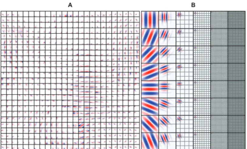
neighborhood have simultaneous activation and similar preferred parameters. Since the neighborhoods overlap, the preferred para-meters of the simple and complex cells change smoothly across the grid graph. Finally, the complex cell responses of the SC model were defined as a static nonlinear function of the locally pooled simple cell energies after model estimation (i.e. total of 625 complex cell responses per patch of size 32×32 pixels and 10000 complex cell responses per image of size 128×128 pixels). The SC model learned topographically organized, spatially local-ized, oriented and bandpass simple and complex cell receptive fields that were similar to those found in the primary visual cortex (Figure 2.2A) (Hubel & Wiesel, 1968; Valois, Albrecht & Thorell, 1982; Jones & Palmer, 1987; Parker & Hawken, 1988).

A B

Figure 2.2: Simple cell receptive fields.A: Simple cell receptive fields of the SC model. Each square is of size 32×32 pixels and shows the inverse weights between the input and a simple cell. The receptive fields were topographically organized, spatially localized, oriented and bandpass, similar to those found in the primary visual cortex.B: Simple cell receptive fields of the GWP model. Each square is of size 128×128 pixels and shows an even-symmetric Gabor wavelet. The grids show the locations of the remaining Gabor wavelets that were used. The receptive fields spanned eight orientations and six spatial frequencies.

(52)

To establish a baseline, we used a GWP model (Daugman, 1985; Jones & Palmer, 1987; Lee, 1996) of 10921 phase-invariant com-plex cells (Kay et al., 2008). Variants of this model were used in a series of seminal encoding and decoding studies (Kay et al., 2008; Naselaris et al., 2009; Nishimoto et al., 2011a; Kay et al., 2013b). Note that the fMRI data set was the same as that in (Kay et al., 2008; Naselaris et al., 2009). Concretely, the GWP model was a hand-designed population of quadrature-phase Gabor wave-lets that spanned a range of locations, orientations and spatial frequencies (Figure 2.2B). Each wavelet was fully connected to the input (i.e. image of size 128×128 pixels). The complex cell responses of the GWP model were defined as a static nonlinear function of the pooled energies of the quadrature-phase wavelets that had the same location, orientation and spatial frequency (i.e. total of 10921 complex cell responses per image of size 128×128 pixels).

Voxel models

To learn the voxel transformation, we used regularized linear regression. The voxel models were estimated from the 1750 feature-transformed stimulus-response pairs in the estimation set by minimizing theL2_{penalized least squares loss function. The}

combination of a voxel model with the complex cells of the SC and GWP models resulted in two encoding models (i.e. SC2 and GWP2 models). The SC2 model linearly pooled the 10000 complex cell responses of the SC model. The GWP2 model linearly pooled the 10921 complex cell responses of the GWP model.

Receptive fields

We first analyzed the receptive fields of the SC model (i.e. simple and complex cell receptive fields). The preferred phase, loca-tion, orientation and spatial frequency of the simple and complex

(53)

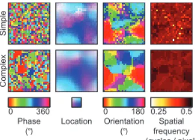
cells were quantified as the corresponding parameters of Gabor wavelets that were fit to their receptive fields. The preferred parameter maps of the simple and complex cells were construc-ted by arranging their preferred parameters on the grid graph (Figure 2.3). Most adjacent simple and complex cells had similar location, orientation and spatial frequency preference, whereas they had different phase preference. In agreement with Hyvärinen and Hoyer (2001), the preferred phase, location and orientation maps reproduced some of the salient features of the columnar organization of the primary visual cortex such as lack of spatial structure (DeAngelis, Ghose, Ohzawa & Freeman, 1999), retino-topy (Hubel & Wiesel, 1977) and pinwheels (Blasdel, 1992), respectively. In contrast to Hyvärinen and Hoyer (2001), the preferred spatial frequency maps failed to reproduce cytochrome oxidase blobs (Tootell, Silverman, Hamilton, Switkes & Valois, 1988). The preferred phase map of the simple cells suggests that

the complex cells are more invariant to phase and location than the simple cells since the complex cells pooled the energies of the simple cells that had different phase preference. To verify the invariance that is suggested by the preferred phase map of the simple cells, the population parameter tuning curves of the simple and complex cells were constructed by fitting Gaussian functions to the median of their responses to Gabor wavelets that had different parameters (Figure 2.4). Like the simple cells, most complex cells were selective to orientation (i.e. standard devi-ation of 21.8° versus 22.9°) and spatial frequency (i.e. standard deviation of 0.52 versus 0.54 in normalized units). Unlike the simple cells, most complex cells were more invariant to phase (i.e. standard deviation of 50.0° versus 158.1°) and location (i.e. standard deviation of 3.70 pixels versus 5.86 pixels). Therefore, they optimally responded to Gabor wavelets that had a specific orientation and spatial frequency, regardless of their phase and exact position.

We then analyzed the receptive fields of the SC2 model (i.e. voxel receptive fields). The eccentricity and size of the

(54)

recept-Location Orientation (°) Phase (°) frequencySpatial (cycles / pixel) 0.25 0.5 0 360 0 180 Simple Complex

Figure 2.3: Preferred parameter maps of the SC model. The phase, location, orientation and spatial frequency preference of the simple and complex cells were quantified as the corres-ponding parameters of Gabor wavelets that were fit to their receptive fields. Each pixel in a parameter map shows the corresponding preferred parameter of a simple or complex cell. The adjacent simple and complex cells had similar location, orientation and spatial frequency preference but different phase preference.

0 16 0 0.5 1 Response 0 0.5 1 Response 0 0.5 1 Response 0 0.5 1 Response Location (D pixels) -16 0 90 Orientation (D °) -90 0 90 Phase (D °) -90 1 10 Spatial frequency (D cycles / pixel) 0.1

Figure 2.4: Population parameter tuning curves of the SC model. The population phase, location, orientation and spatial frequency tunings of the simple (solid lines) and complex cells (dashed lines) were quantified by fitting Gaussian functions to the median of their responses to Gabor wavelets that had dif-ferent parameters. Each curve shows the median of their responses as a function of change in their preferred para-meter. The complex cells were more invariant to phase and location than the simple cells.

ive fields were quantified as the mean and standard deviation of two-dimensional Gaussian functions that were fit to the voxel responses to point stimuli at different locations, respectively. The orientation and spatial frequency tuning of the receptive fields were taken to be the voxel responses to sine-wave gratings that spanned a range of orientations and spatial frequencies. While

(55)

the eccentricity, size and orientation tuning varied across voxels, most voxels were tuned to relatively high spatial frequencies (Fig-ure 2.5Aand Figure 2.5B). The mean predicted voxel responses to sine-wave gratings that had oblique orientations were higher than those that had cardinal orientations and this difference decreased with spatial frequency (Figure 2.5C). While this result is in con-trast to those of the majority of previous single-unit recording and fMRI studies (Mansfield, 1974; Furmanski & Engel, 2000), it is in agreement with those of Swisher et al. (2010). In line withDumoulin and Wandell, 2008; Smith, 2001, the receptive field size systematically increased from V1 to V3 and from low receptive field eccentricity to high receptive field eccentricity (Fig-ure 2.6). The properties of the GWP2 model were similar to those in (Kay et al., 2008). The relationship between the receptive field parameters (i.e. size, eccentricity, area) of the GWP2 model were the same as those of the SC2 model. However, the GWP2 model did not have a large orientation bias.

Encoding

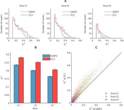
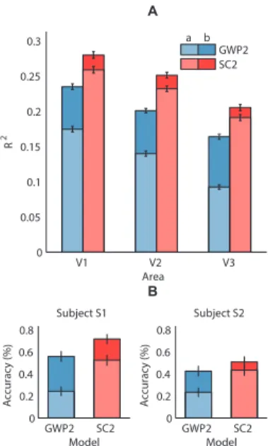
The encoding performance of the SC2 and GWP2 models was defined as the coefficient of determination (R2) between the observed and predicted voxel responses to the 120 images in the validation set across the two subjects. The performance of the SC2 model was found to be significantly higher than that of the GWP2 model (binomial test,p 0.05). Figures 2.7Aand 2.7B

compare the performance of the models across the voxels that survived anR2threshold of 0.1. The meanR2of the SC2 model systematically decreased from 0.28 across 28% of the voxels in V1 to 0.21 across 11% of the voxels in V3. In contrast, the mean

R2_{of the GWP2 model systematically decreased from 0.24 across}

24% of the voxels in V1 to 0.16 across 6% of the voxels in V3. Figure 2.7Ccompares the performance of the models in each voxel. More than 71% of the voxels that did not survive the threshold in each area and more than 92% of the voxels that survived the

(56)

Subject S2, voxel 56220, area V1 x (°) y ( ° ) −10 0 10 −10 −5 0 5 10

Subject S1, voxel 21672, area V3

x (°) y ( ° ) −10 0 10 −10 −5 0 5 10

Orientation (°)

Spatial frequency (cycles /

° ) 0 50 100 150 2 2.5 3

Orientation (°)

° ) 0 50 100 150 2 2.5 3

Orientation (°)

° ) 0 50 100 150 2 2.5 3 Area V1 Orientation (°)

° ) 0 50 100 150 2 2.5 3 A B C 0 0.5 1

Figure 2.5: Receptive fields of the SC2 model. The parameter tuning varied across the voxels and had a bias for high spatial frequencies and oblique orientations. A: Two-dimensional Gaussian functions that were fit to the responses of three representative voxels to point stimuli a