Changing the Face of Database Cloud Services with
Personalized Service Level Agreements
Jennifer Ortiz
†, Victor Teixeira de Almeida
†,§, Magdalena Balazinska
††
Computer Science and Engineering Department, University of Washington Seattle, Washington, USA
§
PETROBRAS S.A., Rio de Janeiro, RJ, Brazil
{jortiz16, valmeida, magda}@cs.washington.edu
ABSTRACT
We develop and evaluate an approach for generatingPersonalized Service Level Agreements(PSLAs) that separate cloud users from the details of compute resources behind a cloud database manage-ment service. PSLAs retain the possibility to trade-off performance for cost and do so in a manner specific to the user’s database.
1.
INTRODUCTION
Over the past several years, cloud service providers have been offering an increasingly large selection of data management ser-vices. Relational Database Service (RDS) and Elastic MapReduce (EMR); Google For example, Amazon Web Services (AWS) [4] in-clude the offers BigQuery [7]; and SQL Server is available through the Windows Azure SQL Database [31]. Accessing a database management system (DBMS) as a cloud service opens the oppor-tunity to re-think the contract between users and the DBMS, es-pecially in the context of data scientists with different skill levels (from data enthusiasts to statisticians) who need to manage and an-alyze their data. Too many services, however, remain too close to the traditional mode of operating a DBMS. In particular, users are expected to select how many instances of the service they wish to purchase and the size of those instances (their CPU and mem-ory resources) [31, 4]. This approach requires users to have the expertise to determine the resource configuration they should use, including advanced notions such as the use of Spot instances [4], which limits how many users cancost-effectivelyleverage a cloud DBMS service to manage and analyze their data.
This problem is not only hard for data scientists, but even for those who are database experts. Although there exist bench-marks [18] that measure the performance on different cloud ser-vices, it is difficult to extrapolate from those benchmarks to the performance for the analysis of a specific database.
More recently, some database services have started to change the mode of interaction with users. Google BigQuery [7], for exam-ple, does not have any notion of service instances. Users execute queries and are charged by the gigabyte of data processed. This interface, however, is not ideal either. It does not offer options to traoff price and performance (only a choice between “on
de-This article is published under a Creative Commons Attribution License (http://creativecommons.org/licenses/by/3.0/), which permits distribution and reproduction in any medium as well allowing derivative works, pro-vided that you attribute the original work to the author(s) and CIDR 2015.
7th Biennial Conference on Innovative Data Systems Research (CIDR ‘15)
January 4-7, 2015, Asilomar, California, USA. Copyright 2015 ACM X-XXXXX-XX-X/XX/XX.
mand” and “reserved” querying). Furthermore, users have no way to predict the performance and, for the case of “on demand” query-ing, the ultimate cost of an analysis.
There has also been research into new SLAs with cloud services. Recent work, however, either requires that users have a pre-defined workload [17, 23] or precise query time constraints [30, 32] with sometimes surprising behaviors such as the rejection of queries un-less they can execute within the SLA threshold [32].
We argue that none of these existing approaches is satisfactory. Cloud services should have a different interface and, fortunately, they have the opportunity to provide it. Instead of showing users the available resources they can lease, or asking users for specific performance requirements for a specific workload, cloud services should show users what is possible with their data and let them pick among those options. The options should come withperformance guaranteesto avoid unexpected behavior. At the same time, they should retain the ability to refine a user’s price-performance options over time.
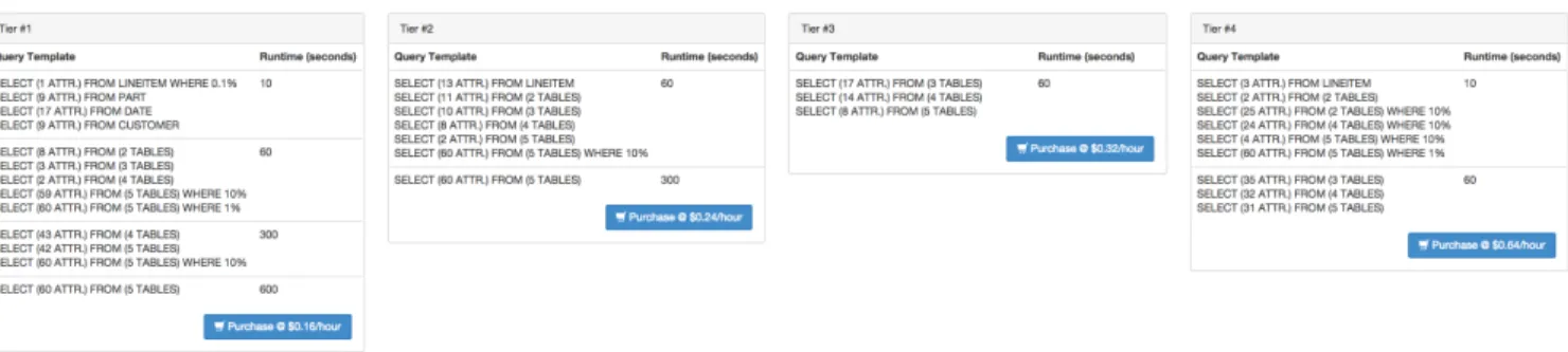
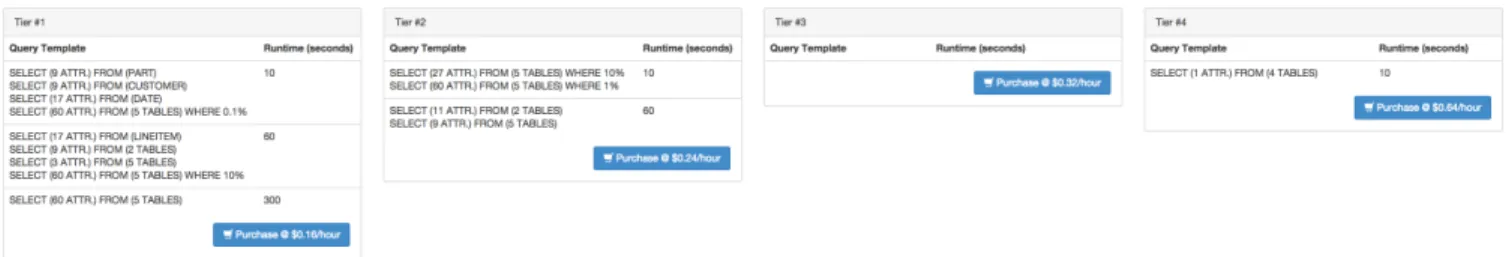
To achieve the above goals, we propose the notion of a Person-alized Service Level Agreement (PSLA). The key idea of the PSLA is for a user to specify the schema of her data and basic statistics (e.g., base table cardinalities) and for the cloud service to show what types of queries the user can run and the performance of these queries with different levels of service, each with a defined cost. The performance is captured with a maximum query runtime while queries are represented with templates. Figure 1 shows an exam-ple PSLA that our service generates (we describe the experimental setup in Section 4). The example shows a PSLA with four tiers generated for the Myria shared-nothing DBMS service [13, 1]. The database to analyze is a 10GB instance of the Star Schema Bench-mark [21]. The PSLA makes cost and performance trade-offs obvi-ous: If a user needs to execute just a few simple selection queries, Tier 1 likely suffices. These queries will run in under 10sec at that tier. Tier 2 significantly improves the runtimes of the most complex join queries compared with Tier 1. Their runtimes go from below 600sec to below 300sec. Tier 3 provides only limited performance improvement compared with Tier 2. Finally, Tier 4 enables queries with small joins to become interactive with runtimes below 10sec. Figure 2 shows a three-tier PSLA for the same dataset but for a single-node SQL Server instance running on Amazon EC2 [5].
In prior work [22], we presented a high-level vision for PSLAs. In this paper, we present thePSLAManager, a new system for the generation and management of PSLAs. More specifically, we make the following contributions:
• In Section 2, we define a model for PSLAs and metrics to as-sess PSLA quality. These metrics include performance error (how accurately the displayed time-thresholds match the ac-tual query times), complexity (a measure of the PSLA size),
Figure 1: Example Personalized Service Level Agreement (PSLA) for a 10GB instance of the Star Schema Benchmark on the shared-nothing Myria DBMS service. These four tiers correspond to 4-node, 6-node, 8-node, and 16-node Myria deployments.
Figure 2: Example Personalized Service Level Agreement (PSLA) for a 10GB instance of the Star Schema Benchmark on a single-node Amazon EC2 instance with SQL Server. The three tiers correspond to a small, medium, and large EC2 instance.
and query capabilities (the types of queries described in the PSLA).
• In Section 3, we develop a method to automatically generate a PSLA for a cloud service and user database. The challenge is to generate PSLAs with low performance error and low complexity at the same time while preserving a given set of query capabilities.
• In Section 4, we show experimentally, using both Ama-zon EC2 [5] and our Myria parallel data management ser-vice [13], that our approach can generate PSLAs with low errors and low complexity.
In Section 5, we discuss future work including the challenges and possible approaches to extending PSLAs to include performance guarantees and physical tuning features.
The PSLAManager generates a PSLA for a given database and cloud service. This system can thus be layered on top of an exist-ing cloud data management service such as Amazon RDS, Amazon Elastic MapReduce, or equivalent. In this paper, we assume such a cloud-specific deployment that gives the PSLAManager access to the cloud service internals including the query optimizer (which we use to collect features of query plans for runtime predictions). However, since the PSLAManager takes as input only the user’s database schema and statistics, it could also be a middleware ser-vice that spans multiple clouds and facilitates the comparison of each service’s price-performance trade-offs through the common PSLA abstraction. The two PSLAs shown in Figures 1 and 2, for example, facilitate the comparison of the Amazon EC2 with SQL
Server service and the Myria service given the user’s database.
2.
PSLA MODEL
We first define a Personalized Service Level Agreement (PSLA) more precisely together with quality metrics for PSLAs.
We start by defining the notion of aquery template. The term “query template” has traditionally been used to refer to parameter-ized queries. Rajaraman et al. [26] used the term query template to designate parameterized queries that differ in their selection pred-icates. Agarwal et al. [2], on the other hand, refer to queries with different projected attributes. We generalize the notion of a query template to select-project-join (SPJ) queries that differ in the pro-jected attributes, relations used in joins (the joined tables are also parameters in our templates), and selection predicates.
Definition 2.1. Query Template: A query template M for a databaseDis a tripleM = (F, S, W)that compactly represents several possible SPJ queries overD: F represents the maximum number of tables in the FROM clause. Srepresents the maximum number of projected attributes in the SELECT clause. W repre-sents the maximum overall query selectivity (as a percent value), based on the predicate in the WHERE clause. Joins are implic-itly represented by PK/FK constraints. No cartesian products are allowed.
For example, the template (4, 12, 10%), represents all queries that joinup tofour tables, project up to 12 attributes, and select up to 10% of the base data in the four tables.
We can now define a Personalized Service Level Agreement: Definition 2.2. Personalized Service Level Agreement: A PSLA for a cloud provider C and user database D is a set of PSLA tiers for the user to choose from, i.e., P SLA(C, D) =
{R1, R2, . . . , Rk}, where each tier,Riis defined as:
Ri= (pi, di,(thi1,{Mi11, Mi12, . . . , Mi1qa}),
(thi2,{Mi21, Mi22, . . . , Mi2qb}),
. . . ,
(thir,{Mir1, Mir2, . . . , Mirqc}) )
Each tier has a fixed hourly price,pi, and no two tiers have the same price. Each tier also has a set of query templatesMi11 throughMirqc clustered intorgroups. Each of these templates
is unique within each tier. Each template group,j, is associated with a time thresholdsthij. Finally,diis the penalty that the cloud agrees to pay the user if a query fails to complete within its corre-sponding time thresholdthij.
Figures 1 and 2 show two example PSLAs for the Star Schema Benchmark [21] dataset. One PSLA is for the Myria shared-nothing cloud service [13] while the other is for the Amazon EC2 service with SQL Server [5] (we describe the experimental setup in Section 4). The figures shows screenshots of the PSLAs as they are shown in our PSLAManager system. To display each template
M = (F, S, W), we convert it into a more easily readable SQL-like format as shown in the figures.
Given a PSLA for a specific cloud service, the user will select a service tierRiand will be charged the corresponding price per time unitpi. The user can then execute queries that follow the templates shown and is guaranteed that all queries complete within the spec-ified time-thresholds (or the cloud provider incurs a penaltydi). Query runtimes across tiers either decrease or stay approximately constant depending on whether the selected configurations (or tiers) improve performance. If some queries take a similar amount of time to process at two tiers of serviceRjandRi, j < i, the queries are shown only for the cheaper tier,Rj: a query that can be ex-pressed through a template from a lower tier,Rj, but has no rep-resentative template in the selected tier,Ri, will execute with the expected runtime shown for the lower tierRj.
There are several challenges related to generating a PSLA: How many tiers should a PSLA have? How many clusters and time-thresholds should there be? How complex should the templates get? To help guide the answers to these questions, we define three metrics to assess the quality of a PSLA:
Definition 2.3. PSLA Complexity Metric: The complexity of a PSLA is measured by the number of query templates that exist in the PSLA for all tiers.
The intuition for the complexity metric is that, ultimately, the size of the PSLA is determined by the number of query templates shown to the user. The smaller the PSLA complexity, the easier it is for the user to understand what is being offered. Hence, we prefer PSLAs that have fewer templates and thus, a lower complexity. Definition 2.4. PSLA Performance Error Metric: The PSLA per-formance error is measured as the root mean squared error (RMSE) between the estimated query runtimes for queries that can be ex-pressed following the PSLA templates in a cluster and the time-thresholds associated with the corresponding cluster. The RMSE is first computed for each cluster. The PSLA error is the average error across all clusters in all tiers.
The RMSE computation associates each query with the template that has the lowest time threshold and that can serve to express the query.
The intuition behind the above error metric is that we want the time thresholds shown in PSLAs to be as close as possible to the ac-tual query runtimes. Minimizing the RMSE means more compact query template clusters, and a smaller difference between query runtime estimates and the time-thresholds presented to the user in the PSLA.
Given a query-template cluster containing queries with expected runtimes {q1, . . . , qk}, and time-thresholdth, the RMSE of the cluster is given by the following equation. Notice that we use rel-ative runtimesbecause queries can differ in runtimes by multiple orders of magnitude. RM SE({q1, . . . , qk}, th) = v u u t1 k k X i=1 qi−th th 2
Because the set of all possible queries that can be expressed fol-lowing a template is large, in our system, we measure the RMSE using only the queries in the workload that our approach generates. Definition 2.5. PSLA Capability Coverage: The class of queries represented by the query templates: e.g., selection queries, selec-tion queries with aggregaselec-tion, full conjunctive queries, conjunctive queries with projection (SPJ queries), conjunctive queries with ag-gregation, union of conjunctive queries, queries with negations.
For this last metric, higher capability coverage is better since it provides users with performance guarantees for more complex queries over their data.
Problem Statement:Given a databaseDand a cloud DBMSC, the problem is how to generate a PSLA comprising a set of PSLA tiersRthat have low complexity, low performance error, and high capability coverage. The challenge is that complexity, performance and capability coverage are at odds with each other. For instance, the higher we extend the capability coverage for the queries, the higher the PSLA complexity becomes and the likelihood of per-formance error increases as well. Additionally, these PSLAs must be generated for a new database each time, or any time the current database is updated. Hence, PSLA generation should be fast.
3.
PSLA GENERATION
We present our approach for generating a PSLA given a database
D and a cloud serviceC. We keep the set of query capabilities fixed and equal to the set of SPJ queries. However, there is no fun-damental limitation that prevents extending the approach to more complex query shapes. Figure 3 shows the overall workflow of the PSLA generation process. We present each step in turn.
We focus on databasesDthat follow a star schema: a fact table
fand a set of dimension tables{d1, . . . , dk}. Queries join the fact table with one or more dimension tables. Star schemas are common in traditional OLAP systems. They are also common in modern analytic applications: A recent paper [2], which analyzed queries at Facebook, found that the most common type of join queries were joins between a single large fact table and smaller dimension tables. It is possible to extend our algorithms to other database schemas, as long as the PK/FK constraints are declared, so that the system can infer the possible joins.
3.1
Tier Definition
The first question that arises when generating a PSLA is what should constitute a service tier? Our approach is to continue to tie service tiers to resource configurations because, ultimately, re-sources are limited and must be shared across users. For example,
Workload Compression into PSLA (repeat for each 9er)
Workload
Genera9on Clustering Query Genera9on Template
Dropping Queries with Similar Times Cloud Service Configurations User Database PSLA Perf. Modeling Tier Selec9on
Figure 3: PSLA generation process.
for Amazon EC2, three natural service tiers correspond to a small, medium, and large instance of that service. For Amazon Elastic MapReduce, possible service tiers are different-size clusters (e.g., cluster of size 2, 3, 4,. . ., 20). We leave it to the cloud provider to set possible resource configurations. Importantly, the cloud can de-fine a large number of possible configurations. The PSLAManager filters-out uninteresting configurations during the PSLA generation process as we describe in Section 3.4. For example, in the case of a shared-nothing cluster, the provider can specify that each cluster size from 1 to 20 is a possible configuration. Our PSLAManager will pick a subset of these configurations to show as service tiers.
The mapping from service tiers to resources is invisible to users. In recent work, it has been shown that cloud providers can often choose different concrete resource configurations to achieve the same application-level performance [16]. The cloud can leverage that flexibility and can also dynamically adjust the resource alloca-tion as we discuss in Secalloca-tion 5. For now, we define each service tier to map onto a specific resource configuration.
3.2
Workload Generation
The first step of PSLA generation is the production of a work-load of queries based on the user’s database. Recall that, in our approach, we do not assume that the user already has a workload. Instead, we only require that the user provides as input a schema and basic statistics on their data. The PSLAManager generates the PSLA from this schema and statistics.
The goal of the PSLA is to show a distribution of query runtimes on the user data. Hence, fundamentally, we want to generate valid queries on the user schema and estimate their runtime for different resource configurations. The key question is, what queries should be included in this process? If we generate too many queries, PSLA generation will become slow and the PSLAs may become complex. If we generate too few queries, they will not sufficiently illustrate performance trade-offs.
From experience working with different cloud DBMS services, we find [22] that, as can be expected, some of the key perfor-mance differences revolve around join processing. Therefore, our approach is to focus on generating queries that illustrate various possible joins based on the user’s data. To avoid generating all possible permutations of tables, we apply the following heuristic: For each pattern of table joins, we generate the query that will pro-cess the largest amount of data. Hence, our algorithm starts from considering each table in isolation. It then considers the fact table joined with the largest dimension table. Next, it generates queries that join the fact table with the two largest dimension tables, and so on until all tables have been joined. The goal is to generate one of the expensive queries among equivalent queries to compute time thresholds that the cloud can more easily guarantee.
Of course, users typically need to look at subsets of the data. Changing the query selectivity can significantly impact the size and thus performance of the joins. To show these trade-offs, we add to each of the above queries selection predicates that retain different orders of magnitude of data such as 0.1%, 1%, 10%, and 100%. To ensure that the predicates change the scales of the join operations, we apply them on the primary key of the fact table.
Finally, since many systems are column-stores, we generate queries that project varying numbers of attributes.
Algorithm 1Query generation algorithm 1: Input:D
2: Q← {},L← {}
3: // Step 1: Generate combinations of tables for the FROM clause
4: foreachti∈Ddo 5: Tq← {t
i} 6: L←L∪Tq
7: // For the fact table add combinations of dimensions tables
8: iftiis the fact table, i.e.ti=fthen
9: Sort{d1, . . . , dk}desc. onsize(di),1≤i≤k 10: foreachj,1≤j≤kdo
11: Dq←take the firstjtables fromD 12: Tq←Tq∪Dq
13: L←L∪Tq
14: // Step 2: Add the projections and selections
15: foreachTq∈Ldo
16: SortA(Tq)desc. onsize(A
j(Tq)),1≤j≤ |A(Tq)| 17: foreachk,1≤k≤ |A(Tq)|do
18: // Project theklargest attributes
19: Aq←take the firstkattributes fromA(Tq) 20: // Add a desired selectivity from a pre-defined set
21: foreacheq∈E T qdo 22: Q←Q∪ {Tq, Aq, eq}
returnQ
Algorithm 1 shows the pseudocode for the query generation step. The input is the databaseD =
{f} ∪ {d1, . . . , dk} , each table
ti ∈D has a set of attributesA(ti). Functionpk(ti)returns the set of primary key attributes forti. The fact tablef has a for-eign key for each dimension table, that references the dimension table’s primary key. The algorithm generates the set of represen-tative queriesQgiven the databaseD. The result setQconsists of triples,(Tq, Aq, eq), whereTqis the set of tables in the FROM clause,Aqis the set of projected attributes in the SELECT clause, andeq
is the desired selectivity value, which translates into a pred-icate on the PK of the fact table in the WHERE clause (or predpred-icate on the PK of a dimension table if there is no fact table in the FROM clause). The algorithm keeps a listLwith all representative sets of tablesTq. Initially every standalone tablet
i ∈Dis inserted as a singleton set intoL(lines 4-6), then the fact table is expanded (line 8), when we generate the joins.
3.3
Query Time Prediction
Given the generated workload, a key building block for our PSLA approach is the ability to estimate query runtimes. Here, we build on extensive prior work [11, 10, 3] and adopt a method based on machine learning: Given a query, we use the cloud ser-vice’s query optimizer to collect query plan features including the estimated query result size and total query plan cost among other features. We build a model offline using a separate star schema dataset. We use that model to predict the runtime of each query in the generated workload given its feature vector and a resource con-figuration. With this approach, to generate a PSLA, users only need to provide the schema of their database and basic statistics such as the cardinality of each input relation.
3.4
Tier Selection
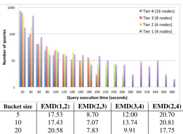
Once our system generates a workload and estimates query run-times for each resource configuration defined by the cloud provider, our approach is to select a small number of these resource config-urations to show as service tiers. Figure 4 illustrates the approach using real query runtime distributions obtained for the 10GB SSB dataset and the Myria service. The figure shows the query runtime distributions (plotted as a histogram with buckets of size 20 sec) for four cluster sizes (4, 6, 8, and 16 nodes). As the figure shows, and as expected, the query runtime distribution shifts to the left with larger Myria clusters. The goal is to narrow down which service
Bucket size EMD(1,2) EMD(2,3) EMD(3,4) EMD(2,4)
5 17.53 8.70 12.00 20.70
10 17.43 7.07 13.74 20.81
20 20.58 7.83 9.91 17.75
Figure 4: Distribution of query times across the four initially con-sidered configurations of Myria. The PSLAManager automatically identifies the tiers with the most different query runtime distribu-tions by computing the Earth Mover’s Distance (EMD) between tiers. EMD(i,j) is the EMD between service tiersiandj.
tiers to show to the user.
Because the goal of the PSLA is to show users different points in the space of price-performance trade-offs, the PSLAManager selects the configurations that differ the most in the distributions of estimated query runtimes for the given workload. To compute these distances, we use the Earth Mover’s Distance [28], since this method effectively compares entire data distributions; in our case, the distribution of query runtimes.
The tier selection algorithm proceeds as follows: Given a sequence of increasingly costly resource configurations:
c1, c2, . . . , ck, we compute the distances EM D(ci, ci+1)∀i ∈
[1, k). We then recursively select the smallest distance in the list and remove the more expensive configurationci+1, and
recom-pute the distance between the new neighborsEM D(ci, ci+2), if
ci+2exists. We terminate once we have a desired numberk0 < k
of tiers. Figure 4 shows the EMD values for different histogram granularities for the Myria example. Assuming a distribution cap-tured with a fine-grained histogram with buckets of size 5sec or 10sec, and assuming the goal is to show only two tiers, the algo-rithm first eliminates the third configuration because EMD(2,3) is the smallest EMD value. It then re-computes EMD(2,4). At this point, EMD(1,2) is smaller than EMD(2,4). As a result, the second configuration is discarded. The final two tiers selected are tier 1 and 4. They correspond to the 4-node and 16-node configurations (we further discuss this figure in Section 4). Observe that the granular-ity with which the query time distributions are captured can affect the choice of service tiers. In this example, if we use buckets of size 20sec, the final two tiers selected are Tiers 1 and 2.
3.5
Workload Compression into Clusters
Our workload-generation approach reduces the set of all possible queries down to a set of representative queries,Q. This set may still easily range in the hundreds of queries as in the case of the SSB schema, for which our approach produces 896 queries.
It would be overwhelming to show the entire list of queries from the generated workload to the user. This would yield PSLAs with low error but high complexity as defined in Section 2. Instead, our approach is to compress the representative workload. The com-pression should reduce the PSLA complexity, which is measured
Figure 5: Clustering techniques illustration. Each X corresponds to a query. (a) Threshold-based clustering (b) Density-based cluster-ing.
by the number of query templates, while keeping the performance error low. These two optimization goals are subject to the constraint that the compression should preserve capability coverage from the original workload: For example, if the original workload includes a query that joins two specific tables, the final query templates should allow the expression of such a query.
Our workload compression approach has three components as shown in Figure 3. The first component is query clustering. We start with the cheapest tier and use a clustering technique to group queries based on their runtimes in that tier. We consider two dif-ferent types of clustering algorithms: threshold-based and density-based. Figure 5 illustrates these two methods.
For threshold-based clustering, we pre-define a set of thresholds and partition queries using these thresholds. The PSLAs shown in Figure 1 and Figure 2 result form this type of clustering. We use two approaches to set the thresholds: (i) we vary the thresh-olds in fixed steps of 10, 100, 300, 500, and 1000 seconds, which we call INTERVAL10, INTERVAL100, INTERVAL300, INTER-VAL500, and INTERVAL1000, respectively; and (ii) we vary the thresholds following different logarithmic scales. One of the scales is based on powers of 10, which we call LOG10. The other one is based on human-oriented time thresholds of 10sec, 1min, 5min, 10min, 30min, and 1hour, which we call LOGHUMAN. These in-tervals are represented by the dashed horizontal lines as seen in Figure 5(a). The benefit of this approach is that the same time-thresholds can serve for all tiers, making them more comparable. However, the drawback is that it imposes cluster boundaries with-out considering the distribution of the query runtimes.
For density-based clustering, we discover clusters of queries within a span of a given amount of seconds. We explore varying the parameter (ε) of the DBSCAN algorithm, in order to discover clusters of queries within a span of 10, 100, 300, 500, and 1000 seconds, which we call DBSCAN10, DBSCAN100, DBSCAN300, DBSCAN500, and DBSCAN1000, respectively. Specifically, we begin with a smallεvalue that produces small clusters throughout a tier. We iterate and slowly increment this value until clusters of the specified size are found. We evaluate and discuss these different clustering algorithms in Section 4.
An example of clusters using the threshold-based and density-based approaches are shown in Figure 5 (a) and (b), respectively. As the figure shows, the choice of the interval[0−10sec]breaks an obvious cluster of queries into two. On the other hand, in the [1−5min]interval, DBSCAN, given the density parameters used, creates two different singleton clusters for two queries inside this
interval, which could arguably be combined into one cluster. For each tier, the generated clusters determine the time-thresholds,thi, that will be shown in the resulting PSLA for the corresponding tier.
3.6
Template Extraction
Once we cluster queries, we compute the smallest set of tem-plates that suffice to express all queries in each cluster. We do so by computing the skyline of queries in each cluster thatdominate
others in terms of query capabilities.
Since the queries that our approach generates vary in the tables they join, the attributes they project, and their overall selectivity, we define the dominance relationship (w) between two queriesqi = (Ti, Ai, ei)andqj= (Tj, Aj, ej)as follows:
qiwqj⇐⇒TiwTj∧AiwAj∧ei⊇ej
which can be read asqidominatesqjiff the set of tables ofqi(Ti) dominates the set of tables ofqj(Tj), the set of attributes ofqi(Ai) dominates the set of attributes ofqj(Aj), and the selectivity ofqi (ei), dominates the selectivity of qj (ej). We say that the set of tablesTidominatesTjiff the number of tables inTiis larger than inTj. Similarly, a set of attributesAidominates another setAjiff the number of attributes inAiis larger than inAj. For selectivities, we simply check whethereiis greater thanej.
We call each query on the skyline aroot query. Given a cluster, for each root queryq, we generate a templateM = (F, S, W), whereFis the number of tables inq’s FROM clause,Sis the num-ber of attribute inq’s SELECT clause, andWis the percent value ofq’ selectivity. For single-table queries, we keep the table name in the template (no table dominance). We do this to help distinguish between the facts table and a dimension table.
Tables 1 and 2 in Section 4 show the reduction in the number of queries shown in PSLAs thanks to the query clustering and tem-plate extraction steps.
3.7
Cross-Tier Compression
Once we generate the PSLA for one tier, we move to the next, more expensive tier. We observe that some queries have similar runtimes across tiers.
As we indicated in Section 2, by choosing one tier, a user gets the level of service of all lower tiers, plus improvements. Hence, if some queries do not improve in performance across tiers, the corre-sponding templates should only be shown in the cheapest tier. Re-call that we measure PSLA complexity by counting the total num-ber of query templates. Hence showing fewer templates improves that quality metric.
Hence, to reduce the complexity of PSLAs, we drop queries from the more expensive tier if their runtimes do not improve compared with the previous, cheaper tier. We call this processcross-tier com-pression. More precisely, queryqjis removed from a tierRj if there exists a queryqiin tierRiwithi < jsuch thatqiwqjand
qj’s runtime inRjfalls within the runtime ofqi’s cluster inRi. We check for dominance instead of finding the exact same query because that query could have previously been removed from the cheaper tier. Tables 1 and 2 in Section 4 show the benefit of this step in terms of reducing the PSLA complexity.
We run the clustering algorithm for the new tier only after the cross-tier compression step.
We also experimented with merging entire clusters between tiers. This approach first computes the query clusters separately for each tier. It then removes clusters from more expensive tiers by merging them with similar clusters in less expensive tiers. A cluster from a more expensive tier is merged only when all of its containing
queries are dominated by queries in the corresponding cluster in the less expensive tier. This approach, however, resulted in a much smaller opportunity for cross-tier compression than the per-query method and we abandoned it.
4.
EVALUATION
We implement the PSLAManager in C# and run it on a 64-bit Windows 7 machine with 8GB of RAM and an Intel i7 3.40GHz CPU. We use the WEKA [12] implementation of the M5Rules [24] technique for query runtime predictions.
We evaluate the PSLAManager approach using two cloud data management services: Amazon EC2 [5] running an instance of SQL Server and our own Myria service [1], which is a shared-nothing parallel data management system running in our private cluster. For Amazon, we use the following EC2 instances as ser-vice tiers: Small (64-bit, 1 ECU, 1.7 GB Memory, Low Network), Medium (64-bit, 2 ECU, 3.75 GB Memory, Moderate Network), and Large (64-bit, 4 ECU, 7.5 GB Memory, Moderate Network). We use the SQL Server Express Edition 2012 provided by each of the machines through an Amazon Machine Image (AMI). For Myria, we use deployments of up to 16 Myria worker processes (a.k.a., nodes) spread across 16 physical machines (Ubuntu 13.04 with 4 disks, 64 GB of RAM and 4 Intel(R) Xeon(R) 2.00 GHz processors). We evaluate the PSLA generation technique across 4 different configurations (4, 6, 8, and 16 nodes) for Myria.
To build the machine learning model to predict query runtimes, we first generate a synthetic dataset using the Parallel Data Gener-ation Framework tool [25]. We use this tool to generate a 10GB dataset that follows a star schema. We call it the PDGF dataset. It includes one fact table and five dimensions tables of different de-grees and cardinalities. The PDGF dataset contains a total of 61 attributes. For our testing dataset, we use a 10GB database gen-erated from the TPC-H Star Schema Benchmark (SSB) [21] with one fact table, four dimension tables and a total of 58 attributes. We choose this dataset size because multiple Hadoop measurement papers report 10GB as a median input dataset analyzed by users today [27].
Since Myria is running in our private cloud, to price the service, we use the prices of the same cluster sizes for the Amazon EMR service [6]. For Amazon, we use prices from single-node Amazon EC2 instances that come with SQL Server installed.
4.1
Concrete PSLAs
We start by looking at the concrete PSLAs that the PSLAMan-ager generates for the SSB dataset and the Amazon and Myria cloud services. Figures 1 and 2 show these PSLAs. The PSLAs use the LOGHUMAN threshold-based clustering method (Section 3.5). We use real query runtimes when generating these PSLAs. We dis-cuss query time prediction errors and their impact on PSLAs in Sections 4.6 and 4.7, where we also show the PSLAs produced when using predicted times (see Figures 9 and 10).
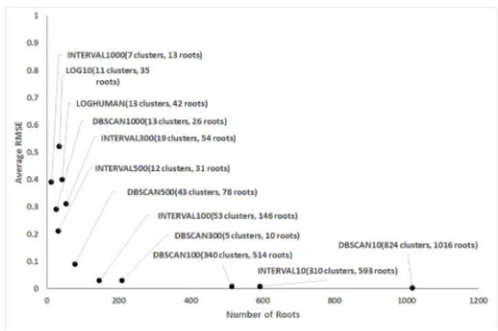
As Figure 1 shows, the PSLA generated for Myria has a low complexity. Each tier has only between 3 and 13 templates grouped into four clusters or less. The PSLA has a total of 32 templates. These few templates represent all SPJ queries for this database (without self joins). The PSLA also has a low average RMSE of 0.20. Most of the error stems from the query distribution in the cheapest tier under threshold 600: All workload queries in that tier and cluster have runtimes below 371sec.
Each service tier corresponds to one of the four Myria cluster configurations, but users need not worry about these resource con-figurations. The price and performance trade-offs are clear: If the user plans to run a few simple selection queries, then Tier 1
suf-fices. These queries will already run in under 10sec at that tier. If the user plans to perform small joins (joining few tables or small subsets of tables), Tier 4 can run such queries at interactive speed, below 10sec. In contrast, if the user will mostly run complex join queries on the entire dataset, then Tier 2 is most cost effective.
Interestingly, the figure also shows that some tiers are more use-ful than others. For example, we can see that Tier 3 improves per-formance only marginally compared with Tier 2. In Section 4.3, we show that the PSLAManager will drop that tier first if requested to generate a 3-tier PSLA.
Figure 2 shows the three-tier PSLA generated for the SSB dataset and the three single-node Amazon instances. This PSLA has more clusters (time thresholds) than the Myria PSLA due to the wider spread in query runtime distributions: 10, 300, 600, 1800, and 3600. Each tier ultimately has between 6 and 17 templates, which is higher than in the Myria PSLA. The total number of templates, however, is interestingly the same. The error for this PSLA is slightly higher with an RMSE of 0.22. Similarly to the Myria PSLA, most of the error comes from the cheapest tier, where more queries happen to fall toward the bottom of the clusters.
Interestingly, the PSLAs not only make the price-performance trade-offs clear for different resource configurations of the same cloud service, they also make cloud services easier to compare. In this example, the PSLAs clearly show that the Myria service is sig-nificantly more cost-effective than the single-node Amazon service for this specific workload and database instance.
Next, we evaluate the different components of the PSLA-generation process individually. We first evaluate the different steps using real query runtimes. We generate the query workload using the algorithm from Section 3.2. For Amazon, we execute all queries from the SSB dataset three times and use the median runtimes to represent the real runtimes. For Myria, we execute all queries for the same dataset only once. In this case, the runtimes have little variance as we run each query on a dedicated cluster and a cold cache. In Section 4.6, we study the query time variance and query time predictions. We examine the impact of using predicted times on the generated PSLAs compared to real runtimes in Section 4.7.
4.2
Workload Generation
Our workload-generation algorithm systematically enumerates specific combinations of SPJ queries and, for each combination, outputs one representative query. With this approach, the work-load remains small: e.g., we generate only 896 queries for the SSB benchmark. However, this approach assumes that the selected query represents the runtime for other similar queries.
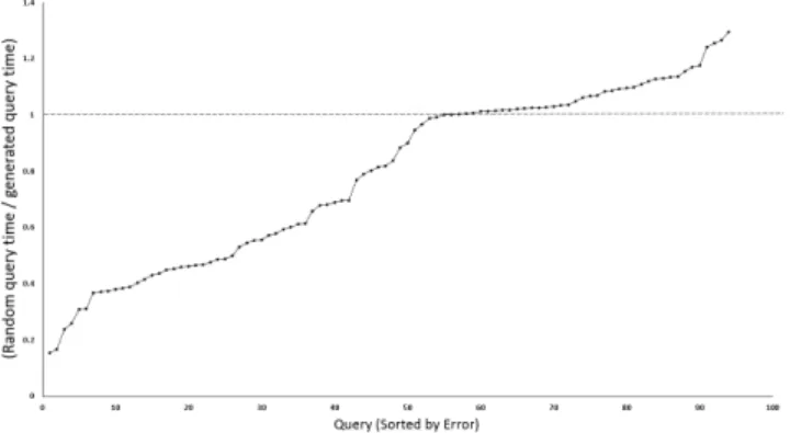
We evaluate the quality of the representative queries that our generator selects by randomly generating 100 queries on the SSB benchmark and associating them with the workload query that is its representative. The representative query should be more expensive to process. We execute the random queries on the Medium EC2 instance and find that he PSLAManager has either a faster runtime or a similar runtime (within 20%) for 90% of the queries. We show these results in Figure 6. This shows that the generated queries are indeed a good representative of the expected upper-bound on the runtime for the user query. The remaining 10% of queries show a limitation of our approach and the need for the cloud to have techniques in place to counteract unexpected query runtimes as we discuss in Section 5.
4.3
Tier Selection
Given a workload of queries with associated query runtimes, the next step of PSLA generation is tier selection. To select tiers, the PSLAManager takes the distribution of query runtimes for all tiers
Figure 6: Runtimes of queries in the generated workloadQ com-pared with 100 random queries on the medium Amazon instance. and computes the earth mover’s distance (EMD) between them. It then eliminates the tiers with the most similar EMD values.
We evaluate this approach for both services. In our experiments, the Myria service has four configurations that correspond to clus-ters of sizes 4, 6, 8, and 16. To capture the query time distributions, we partition the runtimes into buckets of size 5, 10, or 20. We then compute the earth mover’s distance between all consecutive pairs of tiers. Figure 4 shows the runtime distribution with bucket size 20 and the EMD values for all three bucket sizes.
Using EMD identifies that the 6-node and 8-node configurations (Tiers 2 and 3) have the most similar query runtime distributions. If one tier should be removed, our algorithm removes the 8-node configuration (Tier 3). This choice is consistent with the PSLAs shown in Figure 1, where Tier 3 shows only a marginal improve-ment in query runtimes compared with Tier 2.
Once the PSLAManager removes that configuration, the algo-rithm recomputes the EMD between Tier 2 and 4. Here, for bucket sizes 5 or 10, the algorithm removes Tier 2 (6-node configuration) if a second tier should be removed because EMD(2,4)>EMD(1,2). If bucket sizes are coarser-grained at 20 seconds, Tier 4 (the 16-node configuration) gets dropped instead. Using smaller-size buck-ets better approximates the distributions and more accurately se-lects the tiers to remove.
We similarly compute the EMD for the Amazon query run-time distributions using buckets of size 10. We find that EMD(Small,Medium) = 169.10while EMD(Medium,Large) = 23.67. EMD computations with buckets of size 5 yield similar val-ues:168.27and23.75. Our algorithm removes the most expensive tier if we limit the PSLA to only two tiers. This choice is, again, consistent with the small performance gains shown for Tier 3 in Figure 2 compared with Tier 2.
4.4
Workload Clustering and Template
Ex-traction
Once a set ofktiers has been selected, the next step of PSLA generation is workload compression: transforming the distribution of query times into a set of query templates with associated query time thresholds.
In this section, we study the behavior of the 12 different cluster-ing techniques described in Section 3.5 with respect to the PSLA complexity (number of query templates) and performance error (measured as the average RMSE of the relative query times to clus-ter threshold times) metrics. Recall from Section 2 that in order to calculate the error for the PSLA as a whole, we first calculate the RMSE for each individual cluster. Then, we take the average of all these RMSEs across all clusters in all tiers. Again, we use real
Figure 7: PSLA performance error (average RMSE) against com-plexity (# root queries) on Myria considering all four tiers.
query runtimes in this section. Additionally, we disable cross-tier compression. We defer the evaluation of that step to Section 4.5.
Figure 7 and Table 1 show the results for Myria for all four ser-vice tiers. As the figure shows, small fine-grained clusters (INTER-VAL10 and DBSCAN10) give the lowest error on runtime (average RMSE of 0.03 or less), but yield a high complexity based on the number of clusters (92 or more) and templates (233 or more). On the other hand, coarse-grained clusters generate few clusters and templates (only 4 for both INTERVAL1000 and DBSCAN1000) but lead to higher RMSEs (0.93 for INTERVAL1000 and 0.77 for DBSCAN1000). With both methods, interval sizes must thus be tuned to yield a good trade-off. For example, INTERVAL100 yields a small number of clusters and templates (10 clusters and 23 tem-plates) with still achieving a good RMSE value of 0.31. DBSCAN can similarly produce PSLAs with few clusters and templates and a low RMSE, as seen with DBSCAN100. In contrast, LOG10 and LOGHUMAN produce good results similar to the tuned INTER-VAL100 and DBSCAN300 configurations, though with somewhat worse RMSE values, but with no tuning required.
Figure 8 and Table 2 show the results for Amazon. We observe similar trends as for Myria. In general, most of the clustering al-gorithms for the Amazon service have higher complexity but lower RMSE values than the same algorithms for Myria primarily be-cause the query runtimes are more widely spread with the Amazon service. Importantly, the optimal settings for the INTERVAL and DBSCAN methods are different for this service. The best choices are INTERVAL300 or INTERVAL500 and DBSCAN500 or DB-SCAN1000. In contrast, LOG10 and LOGHUMAN still yield a good trade-off between complexity (only 35 and 42 templates re-spectively) and performance error (0.52 and 0.40 rere-spectively).
The key finding is thus that all these clustering techniques have potential to produce clusters with a good performance error and a low complexity. INTERVAL-based and DBSCAN-based tech-niques require tuning. The LOG-based methods yield somewhat worse RMSE metrics but do not require tuning, which makes them somewhat preferable. Additionally, root queries and the associated query templates effectively compress the workload in all but the finest clusters. For example, for the LOG10 clustering methods, the 896 queries are captured with only 35-37 root queries with both services, which correspond to only 4% of the original workload.
4.5
Benefits of Cross-tier Compression
During workload compression, once a tier is compressed into a
Figure 8: PSLA performance error (average RMSE) against com-plexity (# root queries) on Amazon considering all three tiers.
set of clusters and templates, the PSLAManager moves on to the next tier. Before clustering the data at that tier, it drops the queries whose runtimes do not improve,i.e., all queries that fall in the same cluster as in the cheaper tier. In this section, we examine the impact of this cross-tier compression step. Tables 1 and 2 show the result for all 12 clustering methods.
In the case of Myria, we find that cross-tier compression can reduce the number of query templates by up to 75%, as seen for INTERVAL1000. In general, most of the merging occurs from Tier 2 to Tier 1 and from Tier 3 to Tier 1, which confirms the tier se-lection results, where EMD values cause Tier 3 to be dropped first, followed by Tier 2.
In the three-tier Amazon configuration, we find that cross-tier compression can reduce the number of queries by up to 32%. All of the merging occurs between the medium and large tiers only and nothing is merged between the medium and small tiers. This confirms the fact that queries between large and medium tiers have similar runtimes, as computed by the EMD metric in Section 4.3.
As the PSLAManager drops queries whose runtime does not im-prove, the clusters that are created for the higher tiers also have lower RMSE values as shown in Tables 1. and 2
Cross-tier compression is thus an effective tool to reduce PSLA complexity and possibly also PSLA error.
4.6
Query Time Predictions
We now consider the problem of query runtime predictions. We study the implications of errors in query runtime estimates on the generated PSLAs in the next section (Section 4.7).
Accurate query time prediction is a known and difficult problem. This step is not a contribution of this paper. However, we need to evaluate how errors in query time predictions affect the generated PSLA.
Based on prior work [11], we build a machine-learning model (M5Rules) that uses query features from the query optimizer to predict the runtime for each query in our generated workload. We learn the model on the synthetic database generated using the Paral-lel Data Generation Framework tool [25], which we call the PDGF dataset. We then test the learned model on the SSB benchmark database. Both are 10GB in size. We build separate models for Amazon and for Myria.
In the case of Amazon, we learn a model based on features ex-tracted from the SQL Server query optimizer. We use the following features: estimated number of rows in query result, estimated total
Technique Intra-cluster compression only Intra-cluster and cross-tier compression
# of clusters # of query roots RMSE # of clusters # of query roots RMSE
INTERVAL1000 4 4 0.93 1 1 0.90 INTERVAL500 4 4 0.88 1 1 0.82 INTERVAL300 5 7 0.70 3 5 0.33 INTERVAL100 10 23 0.31 10 21 0.10 INTERVAL10 92 233 0.03 90 221 0.01 LOG10 11 37 0.64 9 33 0.46 LOGHUMAN 13 47 0.47 9 32 0.20 DBSCAN10 511 686 0.004 448 605 0.002 DBSCAN100 34 60 0.12 24 50 0.08 DBSCAN300 6 11 0.59 5 10 0.41 DBSCAN500 4 4 0.77 2 2 0.38 DBSCAN1000 4 4 0.77 2 2 0.38
Table 1: Effect of workload compression on Myria. Initial workload comprises 3584 queries (896 queries in 4 tiers).
Technique Intra-cluster compression only Intra-cluster and cross-tier compression
# of clusters # of query roots RMSE # of clusters # of query roots RMSE
INTERVAL1000 7 13 0.39 7 12 0.19 INTERVAL500 12 31 0.21 12 29 0.09 INTERVAL300 19 54 0.31 18 49 0.06 INTERVAL100 53 146 0.03 53 135 0.01 INTERVAL10 310 593 0.008 307 579 0.003 LOG10 11 35 0.52 10 34 0.41 LOGHUMAN 13 42 0.40 10 32 0.22 DBSCAN10 824 1016 0.003 748 941 0.001 DBSCAN100 340 514 0.008 266 429 0.003 DBSCAN300 120 209 0.03 87 142 0.02 DBSCAN500 43 78 0.09 35 64 0.06 DBSCAN1000 13 26 0.29 12 26 0.19
Table 2: Effect of workload compression on Amazon. Initial workload comprises of 2688 queries (896 queries in 3 tiers). IO, estimated total CPU, average row size for query output,
esti-mated total cost. We also add the following features as we found them to improve query time estimates: the number of tables joined in the query, the total size of the input tables, and the selectivity of the predicate that we apply to the fact table.
To build the model, we first use our workload generator to gen-erate 1223 queries for the PDGF database. We then use the SQL Server query optimizer to extract the features for these queries. We finally execute each of these queries on each of the three Amazon configurations (small, medium, and large). We execute each query one time.
In the case of the Amazon cloud, a complicating factor for accu-rate query time prediction is simply the high variance in query run-times in this service. To estimate how much query run-times vary across executions, we run all queries from the SSB benchmark three times on each of the three configurations in Amazon. For each query, we compute the(max(time)max(time)−min(time)) over the three runs. Table 3 shows the average result for all queries. As the table shows, query runtimes can easily vary on average by 15% (small instance) and even 48% (large instance).
This high variance in query times de-emphasizes the need for an accurate query time predictor and emphasizes the need for the cloud service to handle potentially large differences between pre-dicted and actual query times as we discuss further in Section 5.
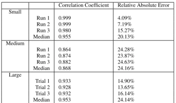
We now evaluate the quality of the query time predictions. Given the large differences in query times across executions, we evaluate the model on each run separately. We also evaluate the predictions on the median runtime across the three executions (separately com-puted for each query). Table 4 shows the results. We plot both the correlation coefficient and the relative absolute error of the model. The correlation coefficient is high for all runs, ranging from 0.864
Configuration Average Runtime Variation
Small 0.149
Medium 0.181
Large 0.481
Table 3: Average variation in query runtimes across three ex-ecutions of all SSB queries for each of the three Amazon in-stances. We compute the runtime variation for each query as
max(time)−min(time)
max(time) across three executions of the query.
to 0.999. The relative absolute error represents how much the pre-dictions improve compared to simply predicting the average. In this case, the lower the percentage, the better. This error ranges from 4% to 24%, with the medium-size instance having the largest prediction errors.
These results show that, for simple queries and without indexes, a simple model can yield good query time predictions. Accurate query time predictions are difficult and, in the cloud, are further complicated by large variations in query times across executions.
We next evaluate query time predictions for the Myria service. Here, the problem is simpler because we measure the runtimes in an isolated setting, where there are no other processes competing for resources on the cluster. Additionally, we measure all query times on a cold cache.
To build the model, we execute each query from the PDGF database once. To test the model, we execute each query from the SSB database once as well. In the case of the Myria service, we partition the fact table across workers and replicate all dimensions tables. As a result, all joins become local joins that get pushed to the PostgreSQL instances, which Myria uses as per-node storage. For the feature vector, we use the same set of features as for Ama-zon plus the estimated query cost from the PostgreSQL optimizer.
Correlation Coefficient Relative Absolute Error Small Run 1 0.999 4.09% Run 2 0.999 7.19% Run 3 0.980 15.27% Median 0.955 20.13% Medium Run 1 0.864 24.28% Run 2 0.874 23.87% Run 3 0.882 24.63% Median 0.868 24.16% Large Trial 1 0.933 14.90% Trial 2 0.928 13.65% Trial 3 0.932 16.14% Median 0.953 24.14%
Table 4: Error on predicted runtimes for each of three runs on Ama-zon and for the median runtime across the runs.
Correlation Relative Absolute Error 4 Workers 0.909 24.05%
6 Workers 0.921 21.79% 8 Workers 0.951 17.24% 16 Workers 0.951 17.24%
Table 5: Error on predicted runtimes for the Myria service. Table 5 shows the results. Interestingly, while the correlation coef-ficients are high, the relative absolute errors are no better than for Amazon. They range between 17% and 24%. These results could likely be significantly improved. For example, our current model does not take into account possible skew in workload across work-ers.
4.7
Effect of Query Time Prediction
Inaccu-racies
Finally, we generate the full PSLAs (all tiers) for both Amazon and Myria using the predicted query times instead of the real run-times. Figures 9 and 10 show the result.
For Myria, the PSLA using predicted times has fewer templates than the PSLA with real runtimes (Figure 1). A closer look at the templates from Figure 9 shows that the query runtimes appear to be underestimated in many cases: Several templates appear with lower time thresholds.
Since query runtimes are underestimated, more merging from the more expensive tiers to the cheaper tiers also occur, resulting in a PSLA with lower complexity. In fact, between these two PSLAs, the number of query templates drops from 32 down to 14.
We observe a similar trend for Amazon with several templates appearing with lower time thresholds and more cross-tier compres-sion in the PSLA based on predicted runtimes. Additionally, for Amazon, the PSLA generally shows more grouping in the query times. Complexity decreases from 32 templates down to 11 be-tween the PSLA that uses real runtimes and the one with predicted runtimes.
Given these results, it is worthwhile to consider the trade-offs be-tween overestimating and underestimating the runtimes for a par-ticular service. If runtimes are slightly overestimated, there are no surprises for the user in terms of queries not meeting their dead-lines. On the other hand, this might hurt the cloud provider since the PSLA will portray runtimes that are slower than what the ser-vice can actually deliver. In contrast, underestimated query times might disappoint the user if queries end up being slower than what the PSLA indicated. We further discuss guaranteeing query times in Section 5.
4.8
PSLA Generation Time
The PSLAManager can generate the concrete PSLAs shown in Figures 9 and 10 in a short amount of time. For Myria, it takes ap-proximately 27sec to generate a PSLA for the SSB dataset. In the Amazon case, it takes an even short amount of time. Only approx-imately 12sec.
Table 6 shows the runtime for each step involved in generating the PSLA for the Myria service. The most expensive step in the PSLA generation is the cross-tier compression step, which takes approximately 19.7sec for the Myria PSLA, or approximately 73% of the total PSLA generation time. Predicting runtimes takes ap-proximately 2sec per tier. In this example, we consider only four tiers. For some services, we could consider many more tiers. For example, all clusters of size 1 through 20, in which case query time prediction could become a significant overhead. We observe, how-ever, that this step is easy to parallelize, which would keep the run-time at 2sec if we simply process all tiers in parallel and lower for an even higher degree of parallelism. For tier selection, it takes less than 2msec to compute each EMD distance using bucket sizes of either 10sec or 5sec. The runtime of this step depends on the total number of buckets, which is small in this scenario. Finally, clus-tering and template extraction is fast when using a threshold-based method such as LOGHUMAN. It only takes 100msec for the most expensive Tier 1. Tier 1 is most expensive because subsequent tiers benefit from cross-tier compression before clustering. Query gen-eration also takes a negligible amount of time compared to the other steps. Only 2msec in total.
We see a similar trend in the Amazon case. Table 7, shows the runtimes for each step in the PSLA process. Query generation takes approximately the same amount of time as in the Myria case, as expected. For predictions, it takes less than 1sec to predict the runtimes for each tier. Amazon is faster since it uses fewer fea-tures to predict the runtimes per query compared with Myria. On the other hand, it takes slightly longer to compute the EMDs for Amazon since the distributions of runtimes per tier are much more widely spread, leading to histograms with larger numbers of buck-ets. Again, the most expensive step is the cross-tier compression. Although it is faster than for the Myria PSLA due to the smaller number of tiers, this step takes approximately 7.5sec or 62% of the PSLA generation time.
5.
DISCUSSION
There are several direct extensions to the initial PSLA genera-tion approach presented in this paper. First, our approach currently assumes no indexes. We posit that physical tuning should happen once the user starts to query the data. The cloud can use existing methods to recommend indexes. It can then re-compute PSLAs but, this time, include the specific queries that the user is running and assume different combination of indexes. This approach, however, requires an extended model for query time prediction and makes it more difficult to compare service tiers with different indexes be-cause each index accelerates different queries.
Second, many variants of the PSLA approach are possible: We could vary the structure of the query templates and the complexity of the queries shown in the PSLAs. We could use different defini-tions for PSLA complexity and error metrics. We could also refine the PSLAs as the user starts to run concrete queries by observing both the queries executed by the user and their performance. Other extensions are also possible.
A third challenge raised by PSLAs relates to query time guar-antees. With our PSLA approach, we argue that cloud services should sell predictable query times in spite of errors in query time estimates and resource sharing across users (a.k.a., tenants), which can cause high variance in query execution times. To guarantee
Figure 9: Example Personalized Service Level Agreement (PSLA) for a 10GB instance of the Star Schema Benchmark and the shared-nothing Myria DBMS service based on predicted runtimes.
Figure 10: Example Personalized Service Level Agreement (PSLA) for a 10GB instance of the Star Schema Benchmark and the single-node Amazon SQL Server instance based on predicted runtimes.
query times, the cloud can use different methods. It can place each tenant in its own set of virtual machines, which correspond to the purchased resources. While this approach isolates tenants well, it limits the flexibility of the cloud in terms of adjusting the resources assigned to a query in case of query time mis-prediction for ex-ample. The cloud can dynamically add VMs when necessary, but doing so during query execution can be expensive as it requires mi-grating state. The approach that seems most promising, and that we are investigating, is to spread user queries evenly across many vir-tual machines and use scheduling to ensure that each user gets on average the amount of resources that he or she purchased, but gets more resources when necessary to meet query time guarantees. The cloud can further leverage algorithms for judicious tenant consoli-dation [16] to minimize interference. The goal is to sell predictable performance to users.
Beyond these fundamental extensions, additional questions re-main: Can the cloud use the PSLAs to help users reason about the cost of different queries? Can it help users to rewrite expensive queries into cheaper, possibly somewhat different, ones? What else should change about the interface between users and the DBMS now that the latter is a cloud service?
6.
RELATED WORK
In prior work [22], we introduced the vision for PSLAs. In this paper, we develop the techniques to generate a PSLA automatically from a given dataset and cloud DBMS.
Admission control frameworks [32, 30, 29] provide techniques to reschedule or even reject queries that cannot meet SLA objec-tives. They use system-wide fixed query performance thresholds. Our work, in contrast, does not reject any queries and PSLAs in-clude different thresholds for different groups of queries and tiers.
Some works present tenant placement optimizations given SLAs [17, 20, 19]. Similarly, Bazaar [16] optimizes cloud re-sources offering a so-calledjob-centric interface, where perfor-mance and cost define the SLOs for user jobs or applications. In our work, instead, we do not fix the SLA objective functions nor
the workload; we show representative query templates with their associated price-performance possibilities (defined by the underly-ing system resources) as a menu for the user to choose from.
The Elastisizer [14] can estimate the performance and cost of a MapReduce workload in different cluster configurations. The ap-proach, however, requires as input the profile from an earlier exe-cution of the workload. PSLAs address the scenarios where neither a prior execution nor even a workload are available.
The idea of representing multiple queries with a single template is not new. The term “query template” is commonly used to refer to parameterized queries differing in their selection predicates [26] or in the projected attributes [2]. We generalize the notion of a query template to include queries that differ in the projected attributes, relations used in joins (the joined tables are also parameters in our templates), and selection predicates.
The work in the literature closest to ours is by Chaudhuri et al. [9, 8], in the context of SQL workload compression. The goal of their work is to compress workloads of queries to improve scalability of tasks such as index selection, without compromising the quality of such tasks’ results. In contrast, our goal is to cluster all possible queries by runtimes and combine queries into templates guarantee-ing coverage in terms of query capabilities. Thus, our optimization goal and workload compression method are different.
Howeet al.[15] looked at the problem of generating sample queries from user databases. Their work is complementary to our workload generation as it infers possible joins between tables, while we assume the presence of a schema with PK-FK constraints.
7.
CONCLUSION
We develop an approach to generate Personalized Service Level Agreements that show users a selection of service tiers with differ-ent price-performance options to analyze their data using a cloud service. We consider the PSLA an important direction for making cloud DMBSs easier to use in a cost-effective manner.
Average Runtime (Milliseconds) Standard Deviation Query Generation 1 Table 0.21 0.40 2 Tables 0.45 0.59 3 Tables 0.98 0.87 4 Tables 1.34 0.58 5 Tables 2.07 0.84 Predictions Tier 1 1313.36 21.01 Tier 1 & 2 2562.98 29.68 Tier 1, 2 & 3 5894.43 69.10 Tier 1, 2, 3 & 4 7501.20 74.72
EMD 38 Buckets (10 sec) 1.5 .002
76 Buckets (5 sec) 0.4 .004
Log-Human Intra-Cluster Compression
Tier 1 102.51 2.68
Tier 2 11.77 0.14
Tier 3 0.006 .0003
Tier 4 1.73 0.02
Log-Human Cross-Tier Compression
Tier 2 to Tier 1 9665.69 69.92 Tier 3 to Tier 1 6733.89 99.00 Tier 4 to Tier 1 3386.46 62.57 Tier 3 to Tier 2 0.87 0.07 Tier 4 to Tier 2 0.91 0.14 Tier 4 to Tier 3 0.46 0.23
Table 6: PSLAManager runtime broken into its main components. The runtimes shown are for the Myria PSLA.
Runtime (Milliseconds) Standard Deviation Query Generation 1 Table 0.23 0.44 2 Tables 0.53 0.53 3 Tables 0.71 0.59 4 Tables 1.37 1.10 5 Tables 1.97 0.94 Predictions Tier 1 859.86 13.720 Tier 1 & 2 1834.76 20.032 Tier 1, 2 & 3 2990.18 34.288
EMD 315 Buckets (10 sec) 68.1 7.3
629 Buckets (5 sec) 527.5 23.2
Log-Human Intra-Cluster Compression
Tier 1 151.60 2.98
Tier 2 61.78 0.83
Tier 3 0.004 0.007
Log-Human Cross-Tier Compression
Tier 2 to Tier 1 3978.60 43.87
Tier 3 to Tier 1 3297.08 70.37
Tier 3 to Tier 2 277.76 4.52
Table 7: PSLAManager runtime broken into its main components. The runtimes shown are for the Amazon PSLA .
8.
ACKNOWLEDGMENTS
This work is supported in part by the National Science Founda-tion through NSF grant IIS-1247469, Petrobras, gifts from EMC, Amazon, and the Intel Science and Technology Center for Big Data. Jennifer Ortiz is also supported by an NSF Graduate Fel-lowship.
9.
REFERENCES
[1] Myria.http://demo.myria.cs.washington.edu.
[2] S. Agarwal et al. BlinkDB: queries with bounded errors and bounded response times on very large data. InEuroSys, pages 29–42, 2013.
[3] M. Akdere, U. Çetintemel, M. Riondato, E. Upfal, and S. B. Zdonik. Learning-based query performance modeling and prediction. InICDE, pages 390–401, 2012.
[4] Amazon AWS.http://aws.amazon.com/. [5] Amazon Elastic Compute Cloud (Amazon EC2).
http://www.amazon.com/gp/browse.html?node=201590011. [6] Amazon Elastic MapReduce (EMR).
http://aws.amazon.com/elasticmapreduce/.
[7] Google BigQuery.https://developers.google.com/bigquery/.
[8] S. Chaudhuri, P. Ganesan, and V. R. Narasayya. Primitives for workload summarization and implications for SQL. InVLDB, pages 730–741, 2003. [9] S. Chaudhuri, A. K. Gupta, and V. R. Narasayya. Compressing SQL workloads.
InSIGMOD, pages 488–499, 2002.
[10] A. Ganapathi, Y. Chen, A. Fox, R. H. Katz, and D. A. Patterson. Statistics-driven workload modeling for the cloud. InICDEW, pages 87–92, 2010.
[11] A. Ganapathi et al. Predicting multiple metrics for queries: Better decisions enabled by machine learning. InICDE, pages 592–603, 2009.
[12] M. Hall, E. Frank, G. Holmes, B. Pfahringer, P. Reutemann, and I. H. Witten. The weka data mining software: An update.SIGKDD Explor. Newsl., 11(1):10–18, Nov. 2009.
[13] D. Halperin, V. T. de Almeida, L. L. Choo, S. Chu, P. Koutris, D. Moritz, J. Ortiz, V. Ruamviboonsuk, J. Wang, A. Whitaker, S. Xu, M. Balazinska, B. Howe, and D. Suciu. Demonstration of the Myria big data management service. InSIGMOD, pages 881–884, 2014.
[14] H. Herodotou, F. Dong, and S. Babu. No one (cluster) size fits all: automatic cluster sizing for data-intensive analytics. InACM Symposium on Cloud Computing in conjunction with SOSP 2011, SOCC ’11, Cascais, Portugal, October 26-28, 2011, page 18, 2011.
[15] B. Howe, G. Cole, N. Khoussainova, and L. Battle. Automatic example queries for ad hoc databases. InSIGMOD, pages 1319–1321, 2011.
tenant-provider gap in cloud services. InSoCC, pages 10:1–10:14, 2012. [17] W. Lang, S. Shankar, J. M. Patel, and A. Kalhan. Towards multi-tenant
performance SLOs. InICDE, pages 702–713, 2012.
[18] A. Li, X. Yang, S. Kandula, and M. Zhang. CloudCmp: comparing public cloud providers. InSIGCOMM, pages 1–14, 2010.
[19] Z. Liu, H. Hacigümüs, H. J. Moon, Y. Chi, and W.-P. Hsiung. PMAX: Tenant placement in multitenant databases for profit maximization. InEDBT, pages 442–453, 2013.
[20] H. A. Mahmoud, H. J. Moon, Y. Chi, H. Hacigümüs, D. Agrawal, and A. El-Abbadi. CloudOptimizer: Multi-tenancy for I/O-bound OLAP workloads. InEDBT, pages 77–88, 2013.
[21] P. E. O’Neil, E. J. O’Neil, X. Chen, and S. Revilak. The star schema benchmark and augmented fact table indexing. InPerformance Evaluation and
Benchmarking (TPCTC), pages 237–252, 2009.
[22] J. Ortiz, V. T. de Almeida, and M. Balazinska. A vision for personalized service level agreements in the cloud. InDanaC, pages 21–25, 2013.
[23] O. Papaemmanouil. Supporting extensible performance slas for cloud databases. InICDEW, pages 123–126, April 2012.
[24] R. J. Quinlan. Learning with continuous classes. InAUS-AI, pages 343–348, Singapore, 1992.
[25] T. Rabl, M. Frank, H. M. Sergieh, and H. Kosch. A data generator for cloud-scale benchmarking. TPCTC’10, pages 41–56, Berlin, Heidelberg. Springer-Verlag.
[26] A. Rajaraman, Y. Sagiv, and J. D. Ullman. Answering queries using templates with binding patterns. InPODS, pages 105–112, 1995.
[27] K. Ren et al. Hadoop’s adolescence: An analysis of hadoop usage in scientific workloads.PVLDB, 6(10):853–864, Aug. 2013.
[28] Y. Rubner et al. The earth mover’s distance as a metric for image retrieval.
International Journal of Computer Vision, 40(2):99–121, 2000.
[29] D. Stamatakis and O. Papaemmanouil. SLA-driven workload management for cloud databases. InICDEW, pages 178–181, 2014.
[30] S. Tozer, T. Brecht, and A. Aboulnaga. Q-Cop: Avoiding bad query mixes to minimize client timeouts under heavy loads. InICDE, pages 397–408, 2010. [31] Windows Azure SQL Database.http:
//www.windowsazure.com/en-us/services/sql-database/. [32] P. Xiong et al. ActiveSLA: a profit-oriented admission control framework for