M
ODEL
C
OMPRESSION VIA
DISTILLATION AND
QUANTIZATION
Antonio Polino ETH Z¨urich [email protected] Razvan Pascanu Google DeepMind [email protected] Dan Alistarh IST Austria [email protected]
ABSTRACT
Deep neural networks (DNNs) continue to make significant advances, solving tasks from image classification to translation or reinforcement learning. One aspect of the field receiving considerable attention is efficiently executing deep models in resource-constrained environments, such as mobile or embedded de-vices. This paper focuses on this problem, and proposes two new compression methods, which jointly leverageweight quantizationanddistillationof larger net-works, called “teachers,” into compressed “student” networks. The first method we propose is calledquantized distillation and leverages distillation during the training process, by incorporating distillation loss, expressed with respect to the teacher network, into the training of a smaller student network whose weights are quantized to a limited set of levels. The second method, differentiable quanti-zation, optimizes thelocation of quantization pointsthrough stochastic gradient descent, to better fit the behavior of the teacher model. We validate both methods through experiments on convolutional and recurrent architectures. We show that quantized shallow students can reach similar accuracy levels to state-of-the-art full-precision teacher models, while providing up to order of magnitude compres-sion, and inference speedup that is almost linear in the depth reduction. In sum, our results enable DNNs for resource-constrained environments to leverage archi-tecture and accuracy advances developed on more powerful devices.
1
INTRODUCTION
Background.Neural networks are extremely effective for solving several real world problems, like image classification (Krizhevsky et al., 2012; He et al., 2016a), translation (Vaswani et al., 2017), voice synthesis (Oord et al., 2016) or reinforcement learning (Mnih et al., 2013; Silver et al., 2016). At the same time, modern neural network architectures are often compute, space and power hungry, typically requiring powerful GPUs to train and evaluate. The debate is still ongoing on whether large models arenecessaryfor good accuracy. It is known that individual network weights can be redundant, and may not carry significant information, e.g. Han et al. (2015). At the same time, large models often have the ability to completely memorize datasets (Zhang et al., 2016), yet they do not, but instead appear to learn generic task solutions. A standing hypothesis for why overcomplete representations are necessary is that they make learning possible by transforming local minima into saddle points (Dauphin et al., 2014) or to discoverrobustsolutions, which do not rely on precise weight values (Hochreiter & Schmidhuber, 1997; Keskar et al., 2016).
If large models are only needed for robustness during training, then significant compression of these models should be achievable, without impacting accuracy. This intuition is strengthened by two related, but slightly different research directions. The first direction is the work ontraining quantized neural networks, e.g. Courbariaux et al. (2015); Rastegari et al. (2016); Hubara et al. (2016); Wu et al. (2016a); Mellempudi et al. (2017); Ott et al. (2016); Zhu et al. (2016), which showed that neural networks can converge to good task solutions even when weights are constrained to having values from a set of integer levels. The second direction aims tocompressalready-trained models, while preserving their accuracy. To this end, various elegant compression techniques have been
proposed, e.g. Han et al. (2015); Iandola et al. (2016); Wen et al. (2016); Gysel et al. (2016); Mishra et al. (2017), which combine quantization, weight sharing, and careful coding of network weights, to reduce the size of state-of-the-art deep models by orders of magnitude, while at the same time speeding up inference.
Both these research directions are extremely active, and have been shown to yield significant com-pression and accuracy improvements, which can be crucial when making such models available on embedded devices or phones. However, the literature on compressing deep networks focuses almost exclusively on finding good compression schemes for a given model, without significantly altering thestructure of the model. On the other hand, recent parallel work (Ba & Caruana, 2013; Hinton et al., 2015) introduces the process ofdistillation, which can be used for transferring the behaviour of a given model to any other structure. This can be used for compression, e.g. to obtain compact representations of ensembles (Hinton et al., 2015). However the size of the student model needs to be large enough for allowing learning to succeed. A model that is too shallow, too narrow, or which misses necessary units, can result in considerable loss of accuracy (Urban et al., 2016).
In this work, we examine whether distillation and quantization can be jointly leveraged for better compression. We start from the intuition that 1) the existence of highly-accurate, full-precision teacher models should be leveraged to improve the performance of quantized models, while 2) quantizing a model can provide better compression than a distillation process attempting the same space gains by purely decreasing the number of layers or layer width. While our approach is very natural, interesting research questions arise when these two ideas are combined.
Contribution.We present two methods which allow the user to compound compression in terms of
depth, by distilling ashallower studentnetwork with similar accuracy to adeeper teachernetwork, with compression in terms ofwidth, by quantizing the weights of the student to a limited set of integer levels, and using less weights per layer. The basic idea is that quantized models can leverage
distillation loss(Hinton et al., 2015), the weighted average between the correct targets (represented by the labels) and soft targets (represented by the teacher’s outputs).
We implement this intuition via two different methods. The first, calledquantized distillation, aims to leverage distillation loss during the training process, by incorporating it into the training of a stu-dent network whose weights are constrained to a limited set of levels. The second method, which we calldifferentiable quantization, takes a different approach, by attempting to converge to theoptimal location of quantization pointsthrough stochastic gradient descent. We validate both methods em-pirically through a range of experiments on convolutional and recurrent network architectures. We show that quantized shallow students can reach similar accuracy levels to full-precision and deeper teacher models on datasets such as CIFAR and ImageNet (for image classification) and OpenNMT and WMT (for machine translation), while providing up to order of magnitude compression, and inference speedup that is linear in the depth.1
Related Work. Our work is a special case ofknowledge distillation(Ba & Caruana, 2013; Hinton et al., 2015), in which we focus on techniques to obtain high-accuracy students that are both quan-tized and shallower. More generally, it can be seen as a special instance oflearning with privileged information, e.g. Vapnik & Izmailov (2015); Xu et al. (2016), in which the student is provided ad-ditional information in the form of outputs from a larger, pre-trained model. The idea of optimizing the locations of quantization points during the learning process, which we use in differentiable quan-tization, has been used previously in Lan et al. (2014); Koren & Sill (2011); Zhang et al. (2017), although in the different context of matrix completion and recommender systems.
Using distillation for size reduction is mentioned in Hinton et al. (2015), for distilling ensembles. To our knowledge, the only other work using distillation in the context of quantization is Wu et al. (2016b), which uses it to improve the accuracy of binary neural networks on ImageNet. We sig-nificantly refine this idea, as we match or even improve the accuracy of the original full-precision model: for example, our 4-bit quantized version of ResNet18 hashigher accuracythan full-precision ResNet18 (matching the accuracy of the ResNet34 teacher): it has higher top-1 accuracy (by>15%) and top-5 accuracy (by>7%) compared to the most accurate model in Wu et al. (2016b).
1
2
PRELIMINARIES
2.1 THEQUANTIZATIONPROCESS
We start by defining ascaling functionsc : Rn →[0,1], which normalizes vectors whose values
come from an arbitrary range, to vectors whose values are in [0,1]. Given such a function, the general structure of the quantization functions is as follows:
Q(v) =sc−1Qˆ(sc(v)), (1) wheresc−1 is the inverse of the scaling function, and Qˆ is the actual quantization function that
only accepts values in[0,1]. We always assumevto be a vector; in practice, of course, the weight vectors can be multi-dimensional, but we can reshape them to one dimensional vectors and restore the original dimensions after the quantization.
Scaling. There are various specifications for the scaling function; in this paper, we will uselinear scaling, e.g. He et al. (2016b), that issc(v) = v−αβ,withα= maxivi−miniviandβ = minivi
which results in the target values being in[0,1], and the quantization function
Q(v) =αQˆ
v−β
α
+β. (2)
Bucketing. One problem with this formulation is that an identical scaling factor is used for the whole vector, whose dimension might be huge. Magnitude imbalance can result in a significant loss of precision, where most of the elements of the scaled vector are pushed to zero. To avoid this, we will usebucketing, e.g. Alistarh et al. (2016), that is, we will apply the scaling function separately to buckets of consecutive values of a certain fixed size. The trade-off here is that we obtain better quantization accuracy for each bucket, but will have to store two floating-point scaling factors for each bucket. We characterize the compression comparison in Section 5. The functionQˆcan also be defined in several ways. We will consider both uniform and non-uniform placement of quantization points.
Uniform Quantization. We fix a parameters ≥ 1, describing the number of quantization levels employed. Intuitively, uniform quantization considerss+ 1equally spaced points between0and1
(including these endpoints). The deterministic version will assign each (scaled) vector coordinatevi
to the closest quantization point, while in the stochastic version we perform rounding probabilisti-cally, such that the resulting value is an unbiased estimator ofvi, of minimal variance.
Formally, the uniform quantization function withs+ 1levels is defined as
ˆ Q(v, s)i= bvisc s + ξi s, (3)
whereξiis the rounding function. For the deterministic version, we defineki =svi− bviscand set
ξi=
1, ifki> 12
0, otherwise, (4)
while for the stochastic version we will setξi ∼ Bernoulli(ki). Note thatki is the normalized
distance between the original pointviand the closest quantization point that is smaller thanviand
that the vector components are quantized independently.
Non-Uniform Quantization.Non-uniform quantization takes as input a set ofsquantization points
{p1, . . . , ps}and quantizes each elementvi to the closest of these points. For simplicity, we only
define thedeterministicversion of this function.
2.2 STOCHASTICQUANTIZATION ISEQUIVALENT TOADDINGGAUSSIANNOISE
In this section we list some interesting mathematical properties of the uniform quantization function. Clearly, stochastic uniform quantization is an unbiased estimator of its input, i.e. E[Q(v)] = v.
What interests us is applying this function to neural networks; as the scalar product is the most common operation performed by neural networks, we would like to study the properties ofQ(v)Tx, wherevis the weight vector of a certain layer in the network andxare the inputs. We are able to show that
Q(v)Tx=vTx+ε (5)
whereεis a random variable that is asymptotically normally distributed, i.e. σ1 nε
D
−→ N(0,1).
Convergence occurs with the dimensionn. For a formal statement and proof, see Section B.1 in the Appendix.
This means that quantizing the weights is equivalent to adding to the output of each layer (before the activation function) a zero-mean error term that is asymptotically normally distributed. The variance of this error term depends on s. This connects quantization to work advocating adding noise to intermediary activations of neural networks as a regularizer (Gulcehre et al., 2016) and to Arora et al. (2018), which investigates the connection between adding noise to a network weights and the network generalization properties. We plan to investigate this connection in more detail in future work.
3
QUANTIZED
DISTILLATION
The context is the following: given a task, we consider a trained state-of-the-art deep model solving it–theteacher, and a compressedstudentmodel. The student is compressed in the sense that 1) it isshallowerthan the teacher; and 2) it isquantized, in the sense that its weights are expressed at limited bit width. The strategy, as for standard distillation (Ba & Caruana, 2013; Hinton et al., 2015) is for the student to leverage the converged teacher model to reach similar accuracy. We note that distillation has been used previously to obtain compact high-accuracy encodings of ensembles (Hin-ton et al., 2015); however, we believe this is the first time it is used for model compression via quantization.
Given this setup, there are two questions we need to address. The first is how to transfer knowledge from the teacher to the student. For this, the student will use thedistillation loss, as defined by Hinton et al. (2015), as the weighted average between two objective functions: cross entropy with soft targets, controlled by the temperature parameterT, and the cross entropy with the correct labels. We refer the reader to Hinton et al. (2015) for the precise definition of distillation loss.
The second question is how to employ distillation loss in the context of aquantizedneural network. An intuitive approach is to rely on projected gradient descent, where a gradient step is taken as in full-precision training, and then the new parameters areprojectedto the set of valid solutions. Critically, we accumulate the error at each projection step into the gradient for the next step. One can think of this process as ifcollecting evidence for whether each weight needs to move to the next quantization point or not. Crucially, the error accumulation prevents the algorithm from get-ting stuck in the current solution if gradients are small, which would occur in a naive projected gradient approach. This is similar to the approach taken by BinaryConnect technique, with some differences. Li et al. (2017) also examines these dynamics in detail. Compared to BinnaryConnect, we use distillation rather than learning from scratch, hence learning more efficiently. We also do not restrict ourselves to binary representation, but rather usevariable bit-widthquantization functions andbucketing, as defined in Section 2.
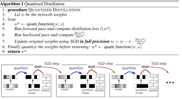
An alternative view of this process, illustrated in Figure 1, is that we perform the SGD step on the
full-precisionmodel, but computing the gradient on thequantized model, expressed with respect to thedistillation loss. See Algorithm 1 for details.
4
DIFFERENTIABLE
QUANTIZATION
4.1 GENERALDESCRIPTION
We introduce differentiable quantization as a general method of improving the accuracy of a quan-tized neural network, by exploiting non-uniform quantization point placement. In particular, we are going to use the non-uniform quantization function defined in Section 2.1. Experimentally, we have
Algorithm 1Quantized Distillation
1: procedureQUANTIZEDDISTILLATION
2: Letwbe the network weights 3: loop
4: wq ←quant function(w, s)
5: Run forward pass and compute distillation lossl(wq)
6: Run backward pass and compute∂l∂w(wqq)
7: Update original weights using SGDin full precisionw=w−ν·∂l∂w(wqq) 8: Finally quantize the weights before returning:wq ←quant function(w, s)
9: returnwq
quantize quantize quantize
SGD step
distil distil SGD step distil SGD step
model quantized model teacher model quantized model teacher model quantized model teacher
Figure 1: Depiction of the steps of quantized distillation. Note the accumulation over multiple steps of gradients in the unquantized model leads to a switch in quantization (e.g. top layer left most square).
found little difference between stochastic and deterministic quantization in this case, and therefore will focus on the simpler deterministic quantization function here.
Letp= (p1, . . . , ps)be the vector of quantization points, and letQ(v, p)be our quantization
func-tion, as defined previously. Ideally, we would like to find a set of quantization points pwhich minimizes the accuracy loss when quantizing the model usingQ(v, p). The key observation is that to find this setp, we can just use stochastic gradient descent, because we are able to compute the gradient ofQwith respect top.
A major problem in quantizing neural networks is the fact that the decision of which pi should
replace a given weight is discrete, hence the gradient is zero: ∂Q(v, p)
∂v = 0, almost everywhere.
This implies that we cannot backpropagate the gradients through the quantization function. To solve this problem, typically a variant of the straight-through estimator is used, see e.g. Bengio et al. (2013); Hubara et al. (2016). On the other hand, the model as a function of the chosen pi
iscontinuousandcan be differentiated; the gradient ofQ(v, p)i with respect topj is well defined
almost everywhere, and it is simply
∂Q(v, p)i
∂pj
=
αi, ifvihas been quantized topj
0, otherwise, (6)
whereαi isi-th element of the scaling factor, assuming we are using a bucketing scheme. If no
bucketing is used, thenαi =αfor everyi. Otherwise it changes depending on which bucket the
weightvibelongs to.
Therefore, we can use the same loss function we used when training the original model, and with Equation (6) and the usual backpropagation algorithm we are able to compute its gradient with respect to the quantization pointsp. Then we can minimize the loss function with respect topwith the standard SGD algorithm. See Algorithm 2 for details.
Note on Efficiency.Optimizing the pointspcan be slower than training the original network, since we have to perform the normal forward and backward pass, and in addition we need to quantize the weights of the model and perform the backward pass to get to the gradients w.r.t.p. However, in our experience differential quantization requires an order of magnitude less iterations to converge to a good solution, and can be implemented efficiently.
Algorithm 2Differentiable Quantization
1: procedureDIFFERENTIABLEQUANTIZATION
2: Letwbe the networks weights andpthe initial quantization points 3: loop
4: wq ←quant function(w, p)
5: Run forward pass and compute lossl(wq)
6: Run backward pass and compute∂l∂w(wqq) 7: Use equation 6 to compute∂l(∂pwq)
8: Update quantization points using SGD or similar:p=p−ν·∂l(∂pwq)
9: returnp
Weight Sharing. Upon close inspection, this method can be related to weight sharing Han et al. (2015). Weight sharing uses ak-mean clustering algorithm to find good clusters for the weights, adopting the centroids as quantization points for a cluster. The network is trained modifying the values of the centroids, aggregating the gradient in a similar fashion. The difference is in the initial assignment of points to centroids, but also, more importantly, in the fact that the assignment of weights to centroids never changes. By contrast, at every iteration we re-assign weights to the closest quantization point, and use a different initialization.
4.2 DISCUSSION ANDADDITIONALHEURISTICS
While the loss is continuous w.r.t. p, there are indirect effects when changing the way each weight gets quantized. This can have drastic effect on the learning process. As an extreme example, we could have degeneracies, where all weights get represented by the same quantization point, making learning impossible. Or diversity ofpigets reduced, resulting in very few weights being represented
at a really high precision while the rest are forced to be represented in a much lower resolution. To avoid such issues, we rely on the following set of heuristics. Future work will look at adding a reinforcement learning loss for how thepiare assigned to weights.
Choose good starting points. One way to initialize the starting quantization points is to make them uniformly spaced, which would correspond to use as a starting point the uniform quantization function. The differentiable quantization algorithm needs to be able to use a quantization point in order to update it; therefore, to make sure every quantization point is used we initialize the points to be the quantiles of the weight values. This ensures that every quantization point is associated with the same number of values and we are able to update it.
Redistribute bits where it matters. Not all layers in the network need the same accuracy. A measure of how important each weight is to the final prediction is the norm of the gradient of each weight vector. So in an initial phase we run the forward and backward pass a certain number of times to estimate the gradient of the weight vectors in each layer, we compute the average gradient across multiple minibatches and compute the norm; we then allocate the number of points associated with each weight according to a simple linear proportion. In short we estimate
E ∂l ∂v 2 (7) wherelis the loss function,vis the vector of weights in a particular layer and ∂v∂l
i= ∂l
∂vi and we use this value to determine which layers are most sensitive to quantization.
When using this process, we will use more than the indicated number of bits in some layers, and less in others. We can reduce the impact of this effect with the use of Huffman encoding, see Section 5; in any case, note that while the total number of points stays constant, allocating more points to a layer will increase bit complexity overall if the layer has a larger proportion of the weights. Use the distillation loss. In the algorithm delineated above, the loss refers to the loss we used to train the original model with. Another possible specification is to treat the unquantized model as the teacher model, the quantized model as the student, and to use as loss the distillation loss between the outputs of the unquantized and quantized model. In this case, then, we are optimizing our quantized model not to perform best with respect to the original loss, but to mimic the results of the unquantized model, which should be easier to learn for the model and provide better results.
Hyperparameter optimization. The algorithm above is an optimization problem very similar to the original one. As usual, to obtain the best results one should experiment with hyperparameters optimization, and different variants of gradient descent.
5
COMPRESSION
We now analyze the space savings when usingbbits and bucket size ofk. Letf be the size of full precision weights (32 bit) and letN be the size of the “vector” we are quantizing. Full precision requiresf Nbits, while the quantized vector requiresbN+2f Nk . (We usebbits per weight, plus the scaling factorsαandβfor every bucket). The size gain is thereforeg(b, k;f) = kbkf+2f.
For differentiable quantization, we also have to store the values of the quantization points. Since this number does not depend onN, the amount of space required is negligible and we ignore it for simplicity. As an example, at256bucket size, using 2 bits per component yields14.2×space savings w.r.t. full precision, while 4 bits yields7.52×space savings. At512bucket size, the 2 bit savings are15.05×, while 4 bits yields7.75×compression.
Huffman encoding.To save additional space, we can use Huffman encoding to represent the quan-tized values. In fact, each quanquan-tized value can be thought as the pointer to a full precision value; in the case of non uniform quantization ispk, in the case of uniform quantization isk/s. We can then
compute the frequency for every index across all the weights of the model and compute the optimal Huffman encoding. The mean bit length of the optimal encoding is the amount of bits we actually use to encode the values. This explains the presence of fractional bits in some of our size gain tables from the Appendix.
We emphasize that we only use these compression numbers as a ballpark figure, since additional implementation costs might mean that these savings are not always easy to translate to practice (Han et al., 2015).
6
EXPERIMENTAL
RESULTS
6.1 SMALL DATASETS
Methods. We will begin with a set of experiments on smaller datasets, which allow us to more carefully cover the parameter space. We compare the performance of the methods described in the following way: we consider as baseline theteachermodel, thedistilledmodel and asmallermodel: the distilled and smaller models have the same architecture, but the distilled model is trained using distillation loss on the teacher, while the smaller model is trained directly on targets. Further, we compare the performance of Quantized Distillation and Differentiable Quantization. In addition, we will also use PM (“post-mortem”) quantization, which uniformly quantizes the weights after training without any additional operation, with and without bucketing. All the results are obtained with a bucket size of 256, which we found to empirically provide a good compression-accuracy trade-off. We refer the reader to Appendix A for details of the datasets and models.
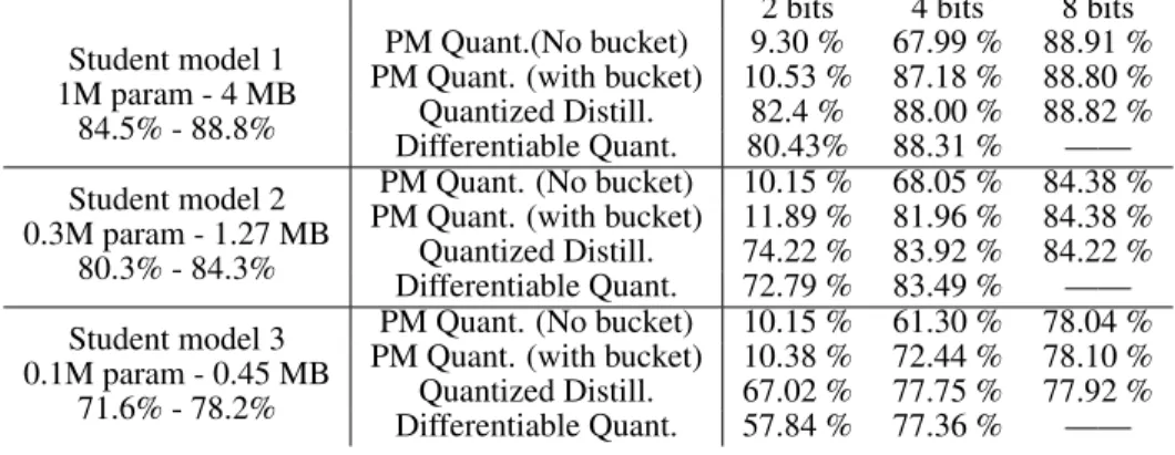
CIFAR-10 Experiments. For image classification on CIFAR-10, we tested the impact of different training techniques on the accuracy of the distilled model, while varying the parameters of a CNN ar-chitecture, such as quantization levels and model size. Table 1 contains the results for full-precision training, PM quantization with and without bucketing, as well as our methods. The percentages on the left below the student models definition are the accuracy of the normal and the distilled model respectively (trained with full precision). More details are reported in table 11 in the appendix. We also tried an additional model where the student is deeper than the teacher, where we obtained that the student quantized to 4 bits is able to achieve significantly better accuracy than the teacher, with a compression factor of more than7×.
We performed additional experiments for differentiable quantization using a wide residual network (Zagoruyko & Komodakis, 2016) that gets to higher accuracies; see table 3.
Overall, quantized distillation appears to be the method with best accuracy across the whole range of bit widths and architectures. It outperforms PM significantly for 2bit and 4bit quantization, achieves accuracy within0.2% of the teacherat 8 bits on the larger student model, and relatively minor accuracy loss at 4bit quantization. Differentiable quantization is a close second on all experiments,
Table 1: CIFAR10 accuracy. Teacher model: 5.3M param, 21 MB, accuracy 89.71 %.Details about the resulting size of the models are reported in table 11 in the appendix.
2 bits 4 bits 8 bits Student model 1
1M param - 4 MB 84.5% - 88.8%
PM Quant.(No bucket) 9.30 % 67.99 % 88.91 % PM Quant. (with bucket) 10.53 % 87.18 % 88.80 % Quantized Distill. 82.4 % 88.00 % 88.82 % Differentiable Quant. 80.43% 88.31 % —— Student model 2
0.3M param - 1.27 MB 80.3% - 84.3%
PM Quant. (No bucket) 10.15 % 68.05 % 84.38 % PM Quant. (with bucket) 11.89 % 81.96 % 84.38 % Quantized Distill. 74.22 % 83.92 % 84.22 % Differentiable Quant. 72.79 % 83.49 % —— Student model 3
0.1M param - 0.45 MB 71.6% - 78.2%
PM Quant. (No bucket) 10.15 % 61.30 % 78.04 % PM Quant. (with bucket) 10.38 % 72.44 % 78.10 % Quantized Distill. 67.02 % 77.75 % 77.92 % Differentiable Quant. 57.84 % 77.36 % ——
Table 2: CIFAR10 accuracy. Teacher model: 5.3M param, 21 MB, accuracy 89.71%. Details about the resulting size of the models are reported in table 14 in the appendix.
2 bits 4 bits Deeper student 5.8M param - 23.2 MB 93.22% - 92.6% PM Quant.(No bucket) 12.60 % 91.11 % PM (with bucketing) 45.82 % 92.30 % Quantized Distilled 89.33 % 92.17 %
Table 3: CIFAR10 accuracy (Wide Residual Network). Teacher model: 145M param, 580 MB, accuracy 95.7 %. Details about the resulting size of the models are reported in table 17 in the appendix.
Student model 2 bits 4 bits
82.7M param - 330 MB 95.3% - 94.19%
PM Quant. (with bucket) 15.35 % 81.1 % Quantized Distill. 94.23 % 94.73 %
but it has much faster convergence. Further, we highlight the good accuracy of the much simpler PM quantization method with bucketing at higher bit width (4 and 8 bits).
CIFAR-100 Experiments. Next, we perform image classification with the full 100 classes. Here, we focus on 2bit and 4bit quantization, and on a single student architecture. The baseline architecture is a wide residual network with 28 layers, and 36.5M parameters, which is state-of-the-art for its depth on this dataset. The student has depth and width reduced by20%, and half the parameters. It is chosen so that reaches the same accuracy as the teacher model when distilled at full precision. Accuracy results are given in Table 4. More details are reported in Table 20, in the appendix.
Table 4: CIFAR100 accuracy and model size. Teacher: 36.5M param, 146 MB, acc. 77.21 %.
2 bits 4 bits
Student model 17.2M param - 68.8 MB
77.08% - 77.24%
PM Quant. (No bucket) 1.38 % - 3.18 MB 1.29 % - 5.77 MB PM Quant. (with bucket) 1.00 % - 3.9 MB 73.5 % - 8.2 MB
Quantized Distill. 27.84 % - 4.3 MB 76.31 % - 8.2 MB Differentiable Quant. 49.32 % - 7.9 MB 77.07 % - 12.4 MB The results confirm the trend from the previous dataset, with distilled and differential quantization preserving accuracy within less than1%at 4bit precision. However, we note that accuracy loss is catastrophic at 2bit precision, probably because of reduced model capacity. We note that differen-tiable quantization is able to best recover accuracy for this harder task.
OpenNMT Experiments. The OpenNMT integration test dataset (Ope) consists of 200K train sentences and 10K test sentences for a German-English translation task. To train and test models we
use the OpenNMT PyTorch codebase (Klein et al., 2017). We modified the code, in particular by adding the quantization algorithms and the distillation loss. As measure of fit we will use perplexity and the BLEU score, the latter computed using the multi-bleu.perl code from the moses project (mos).
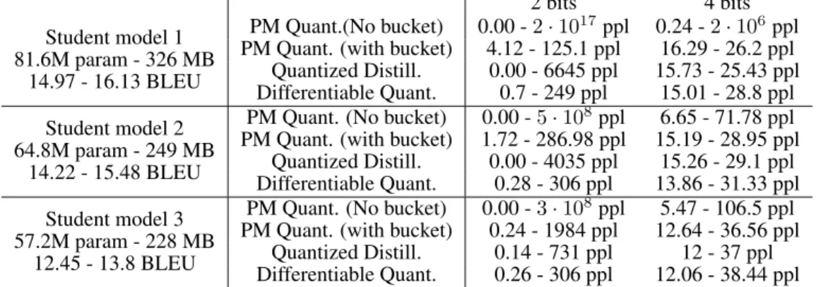
Our target models consist of an embedding layer, an encoder consisting ofnlayers of LSTM, a de-coder consisting ofnlayers of LSTM, and a linear layer. The decoder also uses the global attention mechanism described in Luong et al. (2015). For the teacher network we setn = 2, for a total of 4 LSTM layers with LSTM size500. For the student networks we choosen = 1, for a total of 2 LSTM layers. We vary the LSTM size of the student networks and for each one, we compute the distilled model and the quantized versions for varying bit width. Results are summarized in Table 5. The BLEU scores below the student model refer to the BLEU scores of the normal and distilled model respectively (trained with full precision). Details about the resulting size of the models are reported in table 23 in the appendix.
Table 5: OpenNMT dataset BLEU score and perplexity (ppl). Teacher model: 84.8M param, 340 MB, 26.1 ppl, 15.88 BLEU. Details about the resulting size of the models are reported in table 23 in the appendix. 2 bits 4 bits Student model 1 81.6M param - 326 MB 14.97 - 16.13 BLEU PM Quant.(No bucket) 0.00 -2·1017ppl 0.24 -2·106ppl PM Quant. (with bucket) 4.12 - 125.1 ppl 16.29 - 26.2 ppl
Quantized Distill. 0.00 - 6645 ppl 15.73 - 25.43 ppl Differentiable Quant. 0.7 - 249 ppl 15.01 - 28.8 ppl Student model 2
64.8M param - 249 MB 14.22 - 15.48 BLEU
PM Quant. (No bucket) 0.00 -5·108ppl 6.65 - 71.78 ppl
PM Quant. (with bucket) 1.72 - 286.98 ppl 15.19 - 28.95 ppl Quantized Distill. 0.00 - 4035 ppl 15.26 - 29.1 ppl Differentiable Quant. 0.28 - 306 ppl 13.86 - 31.33 ppl Student model 3
57.2M param - 228 MB 12.45 - 13.8 BLEU
PM Quant. (No bucket) 0.00 -3·108ppl 5.47 - 106.5 ppl
PM Quant. (with bucket) 0.24 - 1984 ppl 12.64 - 36.56 ppl Quantized Distill. 0.14 - 731 ppl 12 - 37 ppl Differentiable Quant. 0.26 - 306 ppl 12.06 - 38.44 ppl A reasonable intuition would be that recurrent neural networks should be harder to quantize than convolutional neural networks, as quantization errors do notaverage outwhen executing repeatedly through the same cell, but accumulate. Results contradict this intuition. In particular, medium and large-sized students are able to essentially recover the same scores as the teacher model on this dataset. Perhaps surprisingly, bucketing PM and quantized distillation perform equally well for 4bit quantization. As expected, cell size is an important indicator for accuracy, although halving both cell size and the number of layers can be done without significant loss.
6.2 LARGER DATASETS
WMT13 Experiments. We run a similar LSTM architecture as above for the WMT13 dataset (Koehn, 2005) (1.7M sentences train, 190K sentences test) and we provide additional ex-periments for quantized distillation technique, see Table 6. We note that, on this large dataset, PM quantization does not perform well, even with bucketing. On the other hand, quantized distillation with 4bits of precision hashigherBLEU score than the teacher, and similar perplexity.
Table 6: WMT13 dataset BLEU score and perplexity (ppl). Teacher model: 84.8M param, 340 MB, 5.8 ppl, 34.7 BLEU. Details about model size are reported in Table 26.
4 bits Student Model
81.6M param - 326 MB 30.22 - 30.21 BLEU
PM Quant. (No bucket) 21.38 BLEU - 12.61 ppl PM Quant. (with bucket) 27.73 BLEU - 7.4 ppl
Quantized Distill. 35.32 BLEU - 6.48 ppl
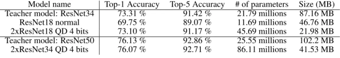
The ImageNet Dataset.We also experiment with ImageNet using the ResNet architecture (He et al., 2016a). In the first experiment, we use a ResNet34 teacher, and a student ResNet18 student model. Experiments quantizing the standard version of this student resulted in an accuracy loss of around
4%, and hence we experiment with a wider model, which doubles the number of filters for each convolutional layer. We call this 2xResNet18. This is in line with previous work on wide ResNet architectures (Zagoruyko & Komodakis, 2016), wide students for distillation (Ba & Caruana, 2013), and wider quantized networks (Mishra et al., 2017). We also note that, in line with previous work on this dataset (Zhu et al., 2016; Mishra et al., 2017), we do not quantize the first and last layers of the models, as this can hurt accuracy.
After 62 epochs of training, the quantized distilled 2xResNet18 with 4 bits reaches avalidation
accuracy of 73.31%. Surprisingly, this is higher than theunquantized ResNet18 model (69.75%), and has virtually the same accuracy as the ResNet34 teacher. In terms of size, this model is more than2×smaller than ResNet18 (but has higher accuracy), and is4×smaller than ResNet34, and about1.5×faster on inference, as it has fewer layers. This is state-of-the-art for 4bit models with 18 layers; to our knowledge, no such model has been able to surpass the accuracy of ResNet18. We re-iterated this experiment using a 4-bit quantized 2xResNet34 student transferring from a ResNet50 full-precision teacher. We obtain a 4-bit quantized student of almost the same accuracy, which is50%shallower and has a2.5×smaller size.
Table 7: Imagenet accuracy and model size. Bucket size = 256.
Model name Top-1 Accuracy Top-5 Accuracy # of parameters Size (MB) Teacher model: ResNet34 73.31 % 91.42 % 21.79 millions 87.16 MB
ResNet18 normal 69.75 % 89.07 % 11.69 millions 46.76 MB
2xResNet18 QD 4 bits 73.10 % 91.17 % 45.69 millions 21.98 MB Teacher model: ResNet50 76.13 % 92.86 % 25.55 millions 102.2 MB 2xResNet34 QD 4 bits 76.07 % 92.71 % 86.11 millions 41.53 MB
6.3 ADDITIONALEXPERIMENTS
Distillation Loss versus Normal Loss.One key question we are interested in is whether distillation loss is a consistently better metric when quantizing, compared to standard loss. We tested this for CIFAR-10, comparing the performance of quantized training with respect to each loss. At 2bit pre-cision, the student converges to67.22%accuracy with normal loss, and to82.40%with distillation loss. At 4bit precision, the student converges to86.01%accuracy with normal loss, and to88.00%
with distillation loss. On OpenNMT, we observe a similar gap: the 4bit quantized student converges to32.67perplexity and15.03BLEU when trained with normal loss, and to25.43perplexity (better than the teacher) and15.73BLEU when trained with distillation loss. This strongly suggests that
distillation loss is superiorwhen quantizing. For details, see Section A.4.1 in the Appendix. Impact of Heuristics on Differentiable Quantization.We also performed an in-depth study of how the various heuristics impact accuracy. We found that, for differentiable quantization, redistributing bits according to the gradient norm of the layers is absolutely essential for good accuracy; quantiles and distillation loss also seem to provide an improvement, albeit smaller. Due to space constraints, we defer the results and their discussion to Section A.4.2 of the Appendix.
Inference Speed.In general, shallower students lead to an almost-linear decrease in inference cost, w.r.t. the depth reduction. For instance, in the CIFAR-10 experiments with the wide ResNet models, the teacher forward pass takes67.4seconds, while the student takes 43.7 seconds; roughly a 1.5x speedup, for 1.75x reduction in depth. On the ImageNet test set using 4 GPUs (data-parallel), a forward pass takes 263 seconds for ResNet34, 169 seconds for ResNet18, and 169 seconds for our 2xResNet18. (So, while having more parameters than ResNet18, it has the same speed because it has the same number of layers, and is not wide enough to saturate the GPU. We note that we did not exploit 4bit weights, due to the lack of hardware support.) Inference on our model is 1.5 times faster, while being 1.8 times shallower, so here the speedup is again almost linear.
7
DISCUSSION
We have examined the impact of combining distillation and quantization when compressing deep neural networks. Our main finding is that, when quantizing, one can (and should) leverage large, accurate models via distillation loss, if such models are available. We have given two methods to do just that, namely quantized distillation, and differentiable quantization. The former acts directly
on the training process of the student model, while the latter provides a way of optimizing the quantization of the student so as to best fit the teacher model.
Our experimental results suggest that these methods can compress existing models by up to an order of magnitude in terms of size, on small image classification and NMT tasks, while preserving accuracy. At the same time, we note that distillation also provides an automatic improvement in
inference speed, since it generates shallower models. One of our more surprising findings is that naive uniform quantizationwith bucketingappears to perform well in a wide range of scenarios. Our analysis in Section 2.2 suggests that this may be because bucketing provides a way to parametrize the Gaussian-like noise induced by quantization. Given its simplicity, it could be used consistently as a baseline method.
In our experimental results, we performed manual architecture search for the depth and bit width of the student model, which is time-consuming and error-prone. In future work, we plan to examine the potential of reinforcement learning or evolution strategies to discover the structure of the student for best performance given a set of space and latency constraints. The second, and more immediate direction, is to examine the practical speedup potential of these methods, and use them together and in conjunction with existing compression methods such as weight sharing Han et al. (2015) and with existing low-precision computation frameworks, such as NVIDIA TensorRT, or FPGA platforms.
ACKNOWLEDGEMENTS
We would like to thank Ce Zhang (ETH Z´urich), Hantian Zhang (ETH Z´urich) and Martin Jaggi (EPFL) for their support with experiments and valuable feedback.
REFERENCES
Opennmt integration testing. https://github.com/OpenNMT/OpenNMT-py. Accessed: 2017-10-25.
Moses baseline. http://www.statmt.org/moses/?n=moses.baseline. Accessed: 2017-10-25.
Dan Alistarh, Jerry Li, Ryota Tomioka, and Milan Vojnovic. Qsgd: Randomized quantization for communication-optimal stochastic gradient descent. arXiv preprint arXiv:1610.02132, 2016. S. Arora, R. Ge, B. Neyshabur, and Y. Zhang. Stronger generalization bounds for deep nets via a
compression approach.ArXiv e-prints, February 2018.
Lei Jimmy Ba and Rich Caruana. Do deep nets really need to be deep? CoRR, abs/1312.6184, 2013. URLhttp://arxiv.org/abs/1312.6184.
Yoshua Bengio, Nicholas L´eonard, and Aaron C. Courville. Estimating or propagating gradients through stochastic neurons for conditional computation. CoRR, abs/1308.3432, 2013. URL http://arxiv.org/abs/1308.3432.
Matthieu Courbariaux, Yoshua Bengio, and Jean-Pierre David. Binaryconnect: Training deep neural networks with binary weights during propagations. CoRR, abs/1511.00363, 2015. URLhttp: //arxiv.org/abs/1511.00363.
Yann Dauphin, Razvan Pascanu, C¸ aglar G¨ulc¸ehre, Kyunghyun Cho, Surya Ganguli, and Yoshua Bengio. Identifying and attacking the saddle point problem in high-dimensional non-convex op-timization. CoRR, abs/1406.2572, 2014. URLhttp://arxiv.org/abs/1406.2572. Caglar Gulcehre, Marcin Moczulski, Misha Denil, and Yoshua Bengio. Noisy activation functions.
InInternational Conference on Machine Learning, pp. 3059–3068, 2016.
Philipp Gysel, Mohammad Motamedi, and Soheil Ghiasi. Hardware-oriented approximation of convolutional neural networks. arXiv preprint arXiv:1604.03168, 2016.
Song Han, Huizi Mao, and William J. Dally. Deep compression: Compressing deep neural network with pruning, trained quantization and huffman coding. CoRR, abs/1510.00149, 2015. URL http://arxiv.org/abs/1510.00149.
Kaiming He, Xiangyu Zhang, Shaoqing Ren, and Jian Sun. Deep residual learning for image recog-nition. InProceedings of the IEEE conference on computer vision and pattern recognition, pp. 770–778, 2016a.
Qinyao He, He Wen, Shuchang Zhou, Yuxin Wu, Cong Yao, Xinyu Zhou, and Yuheng Zou. Effective quantization methods for recurrent neural networks.CoRR, abs/1611.10176, 2016b. URLhttp: //arxiv.org/abs/1611.10176.
G. Hinton, O. Vinyals, and J. Dean. Distilling the Knowledge in a Neural Network. ArXiv e-prints, March 2015.
Sepp Hochreiter and J¨urgen Schmidhuber. Flat minima. Neural Computation, 9(1):1–42, 1997. Itay Hubara, Matthieu Courbariaux, Daniel Soudry, Ran El-Yaniv, and Yoshua Bengio. Quantized
neural networks: Training neural networks with low precision weights and activations. CoRR, abs/1609.07061, 2016. URLhttp://arxiv.org/abs/1609.07061.
Forrest N Iandola, Song Han, Matthew W Moskewicz, Khalid Ashraf, William J Dally, and Kurt Keutzer. Squeezenet: Alexnet-level accuracy with 50x fewer parameters and¡ 0.5 mb model size.
arXiv preprint arXiv:1602.07360, 2016.
Nitish Shirish Keskar, Dheevatsa Mudigere, Jorge Nocedal, Mikhail Smelyanskiy, and Ping Tak Pe-ter Tang. On large-batch training for deep learning: Generalization gap and sharp minima. arXiv preprint arXiv:1609.04836, 2016.
G. Klein, Y. Kim, Y. Deng, J. Senellart, and A. M. Rush. OpenNMT: Open-Source Toolkit for Neural Machine Translation.ArXiv e-prints, 2017.
Philipp Koehn. Europarl: A Parallel Corpus for Statistical Machine Translation. In Conference Proceedings: the tenth Machine Translation Summit, pp. 79–86, Phuket, Thailand, 2005. AAMT, AAMT. URLhttp://www.statmt.org/europarl/.
Yehuda Koren and Joe Sill. Ordrec: an ordinal model for predicting personalized item rating dis-tributions. InProceedings of the fifth ACM conference on Recommender systems, pp. 117–124. ACM, 2011.
Alex Krizhevsky, Ilya Sutskever, and Geoffrey E Hinton. Imagenet classification with deep convo-lutional neural networks. InAdvances in neural information processing systems, pp. 1097–1105, 2012.
Andrew S Lan, Christoph Studer, and Richard G Baraniuk. Matrix recovery from quantized and corrupted measurements. In Acoustics, Speech and Signal Processing (ICASSP), 2014 IEEE International Conference on, pp. 4973–4977. IEEE, 2014.
Hao Li, Soham De, Zheng Xu, Christoph Studer, Hanan Samet, and Tom Goldstein. Training quantized nets: A deeper understanding.CoRR, abs/1706.02379, 2017. URLhttp://arxiv. org/abs/1706.02379.
Minh-Thang Luong, Hieu Pham, and Christopher D. Manning. Effective approaches to attention-based neural machine translation. CoRR, abs/1508.04025, 2015. URLhttp://arxiv.org/ abs/1508.04025.
Naveen Mellempudi, Abhisek Kundu, Dheevatsa Mudigere, Dipankar Das, Bharat Kaul, and Pradeep Dubey. Ternary neural networks with fine-grained quantization. arXiv preprint arXiv:1705.01462, 2017.
Asit K. Mishra, Eriko Nurvitadhi, Jeffrey J. Cook, and Debbie Marr. WRPN: wide reduced-precision networks. CoRR, abs/1709.01134, 2017. URLhttp://arxiv.org/abs/1709.01134. Volodymyr Mnih, Koray Kavukcuoglu, David Silver, Alex Graves, Ioannis Antonoglou, Daan
Wier-stra, and Martin Riedmiller. Playing atari with deep reinforcement learning. arXiv preprint arXiv:1312.5602, 2013.
Aaron van den Oord, Sander Dieleman, Heiga Zen, Karen Simonyan, Oriol Vinyals, Alex Graves, Nal Kalchbrenner, Andrew Senior, and Koray Kavukcuoglu. Wavenet: A generative model for raw audio.arXiv preprint arXiv:1609.03499, 2016.
Joachim Ott, Zhouhan Lin, Ying Zhang, Shih-Chii Liu, and Yoshua Bengio. Recurrent neural net-works with limited numerical precision.arXiv preprint arXiv:1608.06902, 2016.
Mohammad Rastegari, Vicente Ordonez, Joseph Redmon, and Ali Farhadi. Xnor-net: Imagenet classification using binary convolutional neural networks. CoRR, abs/1603.05279, 2016. URL http://arxiv.org/abs/1603.05279.
David Silver, Aja Huang, Chris J Maddison, Arthur Guez, Laurent Sifre, George Van Den Driessche, Julian Schrittwieser, Ioannis Antonoglou, Veda Panneershelvam, Marc Lanctot, et al. Mastering the game of go with deep neural networks and tree search.Nature, 529(7587):484–489, 2016. G. Urban, K. J. Geras, S. Ebrahimi Kahou, O. Aslan, S. Wang, R. Caruana, A. Mohamed, M.
Phili-pose, and M. Richardson. Do Deep Convolutional Nets Really Need to be Deep and Convolu-tional? ArXiv e-prints, March 2016.
Vladimir Vapnik and Rauf Izmailov. Learning using privileged information: similarity control and knowledge transfer. Journal of machine learning research, 16(20232049):55, 2015.
Ashish Vaswani, Noam Shazeer, Niki Parmar, Jakob Uszkoreit, Llion Jones, Aidan N Gomez, Lukasz Kaiser, and Illia Polosukhin. Attention is all you need.arXiv preprint arXiv:1706.03762, 2017.
Wei Wen, Chunpeng Wu, Yandan Wang, Yiran Chen, and Hai Li. Learning structured sparsity in deep neural networks. InAdvances in Neural Information Processing Systems, pp. 2074–2082, 2016.
Jiaxiang Wu, Cong Leng, Yuhang Wang, Qinghao Hu, and Jian Cheng. Quantized convolutional neural networks for mobile devices. InProceedings of the IEEE Conference on Computer Vision and Pattern Recognition, pp. 4820–4828, 2016a.
Xundong Wu, Yong Wu, and Yong Zhao. High performance binarized neural networks trained on the imagenet classification task. CoRR, abs/1604.03058, 2016b. URLhttp://arxiv.org/ abs/1604.03058.
Xinxing Xu, Joey Tianyi Zhou, IvorW Tsang, Zheng Qin, Rick Siow Mong Goh, and Yong Liu. Simple and efficient learning using privileged information. arXiv preprint arXiv:1604.01518, 2016.
S. Zagoruyko and N. Komodakis. Wide Residual Networks. ArXiv e-prints, May 2016.
Chiyuan Zhang, Samy Bengio, Moritz Hardt, Benjamin Recht, and Oriol Vinyals. Understanding deep learning requires rethinking generalization.arXiv preprint arXiv:1611.03530, 2016. Hantian Zhang, Jerry Li, Kaan Kara, Dan Alistarh, Ji Liu, and Ce Zhang. Zipml: Training linear
models with end-to-end low precision, and a little bit of deep learning. InInternational Confer-ence on Machine Learning, pp. 4035–4043, 2017.
Chenzhuo Zhu, Song Han, Huizi Mao, and William J. Dally. Trained ternary quantization. CoRR, abs/1612.01064, 2016. URLhttp://arxiv.org/abs/1612.01064.
A
FULL EXPERIMENTAL RESULTS
A.1 CIFAR10The model used to train CIFAR10 is the one described in Urban et al. (2016) with some minor mod-ifications. We use standard data augmentation techniques, including random cropping and random flipping. The learning rate schedule follows the one detailed in the paper. The structure of the mod-els we experiment with consists of some convolutional layers, mixed with dropout layers and max pooling layers, followed by one or more linear layers.
The model used are defined in Table 8. Thecindicates a convolutional layer, mp a max pooling layer, dp a dropout layer, fc a linear (fully connected) layer. The exponent indicates how many consecutive layers of the same type are there, while the number in front of the letter determines the size of the layer. In the case of convolutional layers is the number of filters. All convolutional layers of the teacher are 3x3, while the convolutional layers in the smaller models are 5x5.
Table 8: CIFAR10: model specifications
Teacher model 76c2-mp-dp-126c2-mp-dp-148c4-mp-dp-1200fc-dp-1200fc
Smaller model 1 75c-mp-dp-50c2-mp-dp-25c-mp-dp-500fc-dp Smaller model 2 50c-mp-dp-25c2-mp-dp-10c-mp-dp-400fc-dp Smaller model 3 25c-mp-dp-10c2-mp-dp-5c-mp-dp-300fc-dp
Following the authors of the paper, we don’t use dropout layers when training the models using distillation loss. Distillation loss is computed with a temperature ofT = 5.
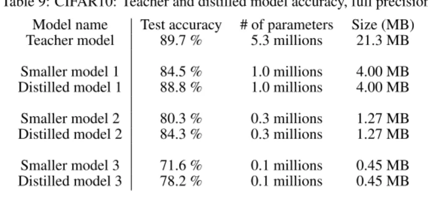
Table 9 reports the accuracy of the models trained (in full precision) and their size. Table 10 reports the accuracy achieved with each method, and table 11 reports the optimal mean bit length using Huffman encoding and resulting model size.
Table 9: CIFAR10: Teacher and distilled model accuracy, full precision Model name Test accuracy # of parameters Size (MB) Teacher model 89.7 % 5.3 millions 21.3 MB Smaller model 1 84.5 % 1.0 millions 4.00 MB Distilled model 1 88.8 % 1.0 millions 4.00 MB Smaller model 2 80.3 % 0.3 millions 1.27 MB Distilled model 2 84.3 % 0.3 millions 1.27 MB Smaller model 3 71.6 % 0.1 millions 0.45 MB Distilled model 3 78.2 % 0.1 millions 0.45 MB
Table 10: CIFAR10: Test accuracy for quantized models. Results computed with bucket size = 256 2 bits 4 bits 8 bits
PM Quant. 1 (No bucket) 9.30 % 67.99 % 88.91 % PM Quant. 1 (with bucket) 10.53 % 87.18 % 88.80 % Quantized Distill. 1 82.4 % 88.00 % 88.82 % Differentiable Quant. 1 80.43% 88.31 % — PM Quant. 2 (No bucket) 10.15 % 68.05 % 84.38 % PM Quant. 2 (with bucket) 11.89 % 81.96 % 84.38 % Quantized Distill. 2 74.22 % 83.92 % 84.22 % Differentiable Quant. 2 72.79 % 83.49 % — PM Quant. 3 (No bucket) 10.15 % 61.30 % 78.04 % PM Quant. 3 (with bucket) 10.38 % 72.44 % 78.10 % Quantized Distill. 3 67.02 % 77.75 % 77.92 % Differentiable Quant. 3 57.84 % 77.36 % —
We also performed an experiment with a deeper student model. The architecture is76c3
-mp-dp-126c3-mp-dp-148c5-mp-dp-1000fc-dp-1000fc-dp-1000fc (following the same notation as in table
8). We use the same teacher as in the previous experiments. Results are in table 13. A.1.1 CIFAR10 - WIDERESNET ARCHITECTURE
For our second set of experiments on CIFAR10 with the WideResNet architecture, see table 15. Note that we increase the number of filters but reduce the depth of the model. The implementation of WideResNet used can be found on GitHub2. Results of quantized methods are in table 16 while the size of the resulting models is detailed in table 17.
Table 11: CIFAR10: Optimal length Huffman encoding and resulting model size. Bucket size = 256
2 bits 4 bits 8 bits
PM Quant. 1 (No bucket) 1.34 bits - 0.17 MB 2.43 bits - 0.3 MB 6.48 bits - 0.81 MB PM Quant. 1 (with bucket) 1.58 bits - 0.22 MB 3.52 - 0.47 MB 7.58 bits - 0.98 MB Quantized Distill. 1 1.7 bits - 0.24 MB 3.64 bits - 0.48 MB 7.70 bits - 1 MB Differentiable Quant. 1 3.18 bits - 0.43 MB 5.34 bits - 0.7 MB —— PM Quant. 2 (No bucket) 1.43 bits - 0.05 MB 2.6 bits - 0.1 MB 6.65 bits - 0.26 MB PM Quant. 2 (with bucket) 1.6 bits - 0.07 MB 3.58 bits - 0.15 MB 7.64 bits - 0.31 MB Quantized Distill. 2 1.7 bits - 0.08 MB 3.55 bits - 0.15 MB 7.64 bits - 0.31 MB Differentiable Quant. 2 3.16 bits - 0.13 MB 5.34 bits - 0.22 MB —— PM Quant. 3 (No bucket) 1.46 bits - 0.02 MB 2.62 bits - 0.03 MB 6.66 bits - 0.09 MB PM Quant. 3 (with bucket) 1.58 bits - 0.026 MB 3.51 bits - 0.053 MB 7.56 bits - 0.1 MB
Quantized Distill. 3 1.64 bits - 0.027 MB 3.53 bits - 0.053 MB 7.59 bits - 0.11 MB Differentiable Quant. 3 3.12 bits - 0.04 MB 5.41 bits - 0.08 MB ——
Table 12: CIFAR10: Teacher and distilled model accuracy, full precision Model name Test accuracy # of parameters Size (MB)
Teacher model 89.7 % 5.3 millions 21.3 MB
Deeper normal model 1 93.22 % 5.8 millions 23.40 MB Deeper distilled model 1 92.60 % 5.8 millions 23.40 MB
Table 13: CIFAR10: Test accuracy for quantized deeper student model. Results computed with bucket size = 256
2 bits 4 bits PM Quant. (No bucket) 12.60 % 91.11 % PM Quant. (with bucket) 45.82 % 92.30 % Quantized Distill. 89.33 % 92.17 %
Table 14: CIFAR10: Optimal length Huffman encoding and resulting model size for deeper student model. Bucket size = 256
2 bits 4 bits
PM Quant. (No bucket) 1.50 bits - 1.13 MB 3.21 bits - 2.38 MB PM Quant. (with bucket) 1.82 bits - 1.55 MB 3.92 bits - 3.07 MB Quantized Distill. 1.84 bits - 1.56 MB 3.92 bits - 3.08 MB
Table 15: CIFAR10: Teacher and distilled model accuracy, full precision, wide resnet Model name Structure Test accuracy # of parameters Size (MB) Teacher model depth = 28, wide factor = 20 95.74 % 145 millions 580 MB Smaller model depth = 22, wide factor = 16 95.19 % 82.7 millions 330 MB Distilled model depth = 22, wide factor = 16 94.19 % 82.7 millions 330 MB
A.2 CIFAR100
For our CIFAR100 experiments, we use the same implementation of wide residual networks as in our CIFAR10 experiments. The wide factor is a multiplicative factor controlling the amount of filters in each layer; for more details please refer to the original paper Zagoruyko & Komodakis (2016). We train for 200 epochs with an initial learning rate of 0.1.
Table 16: CIFAR10: Test accuracy for quantized models. Results computed with bucket size = 256 2 bits 4 bits
PM Quant. (with bucket) 15.35 % 81.09 % Quantized Distill. 94.23 % 94.73 %
Table 17: CIFAR10: Optimal length Huffman encoding and resulting model size. Bucket size = 256
2 bits 4 bits
PM Quant. (with bucket) 1.44 bits - 17.56 MB 2.62 bits - 29.75 MB Quantized Distill. 1.54 bits - 17.81 MB 3.48 bits - 38.65 MB
For the CIFAR100 experiments we focused on one student model. Distillation loss is computed with a temperature ofT = 5.
Table 18: CIFAR100: Teacher and distilled model accuracy, full precision
Model name Structure Test accuracy # of parameters Size (MB) Teacher model depth = 28, wide factor = 10 77.21 % 36.5 millions 146 MB Smaller model depth = 22, wide factor = 8 77.08 % 17.2 millions 68.8 MB Distilled model depth = 22, wide factor = 8 77.24 % 17.2 millions 68.8 MB
Table 19: CIFAR100: Test accuracy for quantized models. Results computed with bucket size = 256 2 bits 4 bits
PM Quant. (No bucket) 1.38% 1.29% PM Quant. (with bucket) 1.00 % 73.47%
Quantized Distill. 27.84% 76.31% Differentiable Quant. 49.32% 77.07%
Table 20: CIFAR100: Optimal length Huffman encoding and resulting model size. Bucket size = 256
2 bits 4 bits
PM Quant. (No bucket) 1.47 bits - 3.18 MB 2.68 bits - 5.77 MB PM Quant. (with bucket) 1.56 bits - 3.90 MB 3.55 bits - 8.18 MB Quantized Distill. 1.73 bits - 4.27 MB 3.54 bits - 8.16 MB Differentiable Quant. 3.23 bits - 7.84 MB 5.53 bits - 12.44 MB
A.3 OPENTNMTINTEGRATION TEST DATASET
As mentioned in the main text, we use the openNMT-py codebase. We slightly modify it to add distillation loss and the quantization methods proposed. We mostly use standard options to train the model; in particular, the learning rate starts at 1 and is halved every epoch starting from the first epoch where perplexity doesn’t drop on the test set. We train every model for 15 epochs. Distillation loss is computed with a temperature ofT = 1.
A.4 WMT13DATASET
For the WMT13 datasets, we run a similar architecture. We ran all models for 15 epochs; the smaller model overfit with 15 epochs, so we ran it for 5 epochs instead.
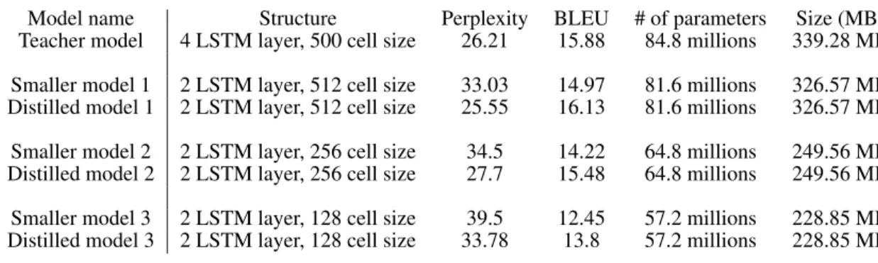
Table 21: openNMT integ: Teacher and distilled models perplexity and BLEU, full precision
Model name Structure Perplexity BLEU # of parameters Size (MB)
Teacher model 4 LSTM layer, 500 cell size 26.21 15.88 84.8 millions 339.28 MB Smaller model 1 2 LSTM layer, 512 cell size 33.03 14.97 81.6 millions 326.57 MB Distilled model 1 2 LSTM layer, 512 cell size 25.55 16.13 81.6 millions 326.57 MB Smaller model 2 2 LSTM layer, 256 cell size 34.5 14.22 64.8 millions 249.56 MB Distilled model 2 2 LSTM layer, 256 cell size 27.7 15.48 64.8 millions 249.56 MB Smaller model 3 2 LSTM layer, 128 cell size 39.5 12.45 57.2 millions 228.85 MB Distilled model 3 2 LSTM layer, 128 cell size 33.78 13.8 57.2 millions 228.85 MB
Table 22: openNMT integ: Test accuracy for quantized models. Results computed with bucket size = 256
2 bits 4 bits
PM Quant. 1 (No bucket) 2·1017ppl - 0.00 BLEU 2.7·106ppl - 0.24 BLEU
PM Quant. 1 (with bucket) 125.1 ppl - 4.12 BLEU 26.21 ppl - 16.29 BLEU Quantized Distill. 1 6645 ppl - 0.00 BLEU 25.43 ppl - 15.73 BLEU Differentiable Quant. 1 249 ppl - 0.7 BLEU 28.8 ppl - 15.01 BLEU PM Quant. 2 (No bucket) 5·108ppl - 0.00 BLEU 71.78 ppl - 6.65 BLEU PM Quant. 2 (with bucket) 286.98 ppl - 1.72 BLEU 28.95 ppl - 15.19 BLEU
Quantized Distill. 2 4035 ppl - 0.00 BLEU 29.1 ppl - 15.26 BLEU Differentiable Quant. 2 306 ppl - 0.28 BLEU 31.33 ppl - 13.86 BLEU PM Quant. 3 (No bucket) 3·108ppl - 0.00 BLEU 106.5 ppl - 5.47 BLEU
PM Quant. 3 (with bucket) 1984 ppl - 0.24 BLEU 36.56 ppl - 12.64 BLEU Quantized Distill. 3 731 ppl - 0.14 BLEU 37 ppl - 12 BLEU Differentiable Quant. 3 306 ppl - 0.26 BLEU 38.4 ppl - 12.06 BLEU
Table 23: openNMT integ: Optimal length Huffman encoding and resulting model size. Bucket size = 256
2 bits 4 bits
PM Quant. 1 (No bucket) 1.36 bits - 13.93 MB 1.77 bits - 18.10 MB PM Quant. 1 (with bucket) 1.65 bits - 19.47 MB 3.69 bits - 40.26 MB Quantized Distill. 1 1.75 bits - 20.4 MB 3.66 bits - 39.97 MB Differentiable Quant. 1 1.72 bits - 20.1 MB 4.38 bits - 47.32 MB PM Quant. 2 (No bucket) 1.34 bits - 10.89 MB 1.86 bits - 15.09 MB PM Quant. 2 (with bucket) 1.65 bits - 15.4 MB 3.68 bits - 31.91 MB Quantized Distill. 2 1.85 bits - 17.05 MB 3.68 bits - 31.91 MB Differentiable Quant. 2 1.93 bits - 17.67 MB 4.17 bits - 35.83 MB PM Quant. 3 (No bucket) 1.47 bits - 10.54 MB 2.13 bits - 15.24 MB PM Quant. 3 (with bucket) 1.65 bits - 13.6 MB 3.68 bits - 28.14 MB Quantized Distill. 3 1.86 bits - 15.13 MB 3.68 bits - 28.18 MB Differentiable Quant. 3 1.99 bits - 16.04 MB 4.25 bits - 31.18 MB
A.4.1 DISTILLATION VERSUSSTANDARDLOSS FORQUANTIZATION
In this section we highlight the positive effects of using distillation loss during quantization. We take models with the same architecture and we train them with the same number of bits; one of the models is trained with normal loss, the other with the distillation loss with equal weighting between soft cross entropy and normal cross entropy (that is, it is the quantized distilled model).
Table 24: WMT13: Teacher and distilled models perplexity and BLEU, full precision
Model name Structure Perplexity BLEU # of parameters Size (MB)
Teacher model 4 LSTM layer, 500 cell size 5.83 34.77 84.8 millions 339.28 MB Smaller model 1 2 LSTM layer, 500 size 7.98 30.22 80.8 millions 323.25 MB Distilled model 1 2 LSTM layer, 550 cell size 7.18 30.21 84.3 millions 337.21 MB
Table 25: WMT13: Test accuracy for quantized models. Results computed with bucket size = 256 4 bits
PM Quant. (No bucket) 12.17 ppl - 22.79 BLEU PM Quant. (with bucket) 7.34 ppl - 26.18 BLEU
Quantized Distill. 6.48 ppl - 35.32 BLEU
Table 26: WMT13: Optimal length Huffman encoding and resulting model size. Bucket size = 256 4 bits
PM Quant. 1 (No bucket) 1.98 bits - 20.92 MB PM Quant. 1 (with bucket) 3.63 bits - 41.02 MB Quantized Distill. 1 3.65 bits - 41.16 MB
Table 27 shows the results on the CIFAR10 dataset; the models we train have the same structure as the Smaller model 1, see Section A.1.
Table 28 shows the results on the openNMT integration test dataset; the models trained have the same structure of Smaller model 1, see Section A.3. Notice that distillation loss can significantly improve the accuracy of the quantized models.
Table 27: CIFAR10: Distillation loss vs normal loss when quantizing 2 bits 4 bits
Normal loss 67.22 % 86.01 % Distillation loss 82.40% 88.00%
Table 28: openNMT integ: Distillation loss vs normal loss when quantizing 4 bits
Normal loss 32.67 ppl 15.03 BLEU Distillation loss 25.43 ppl 15.73 BLEU
These results suggest that quantization works better when combined with distillation, and that we should try to take advantage of this whenever we are quantizing a neural network.
A.4.2 DIFFERENT HEURISTICS FOR DIFFERENTIABLE QUANTIZATION
To test the different heuristics presented in Section 4.2, we train with differentiable quantization the Smaller model 1 architecture specified in Section A.1 on the cifar10 dataset. The same model is trained with different heuristics to provide a sense of how important they are; the experiments is performed with 2 and 4 bits.
Results suggests that when using 4 bits, the method is robust and works regardless. When using 2 bits, redistributing bits according to the gradient norm of the layers is absolutely essential for this method to work ; quantiles starting point also seem to provide an small improvement, while using distillation loss in this case does not seem to be crucial.
Table 29: Results with automatically redistributed bits Quantiles Uniform 2 bits Distillation loss 82.94 % 78.76 % Normal loss 83.67 % 76.60 % 4 bits Distillation loss 88.93 % 88.50 % Normal loss 88.80 % 88.74 %
Table 30: Results without automatically redistributed bits Quantiles Uniform 2 bits Distillation loss 19.69 % 22.81 % Normal loss 25.28 % 22.11 % 4 bits Distillation lossNormal loss 88.39 %88.43 % 88.67 %88.44 %
B
QUANTIZATION IS
EQUIVALENT TO
ASYMPTOTICALLY
NORMALLY
DISTRIBUTED
NOISE
In this section we will prove some results about the uniform quantization function, including the fact that is asymptotically normally distributed, see subsection B.1 below. Clearly, we refer to the stochastic version, see Section 2.1.
Unbiasedness
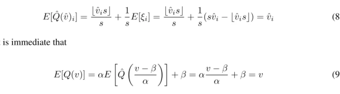
We first start proving the unbiasedness ofQˆ;
E[ ˆQ(ˆv)i] = bvˆisc s + 1 sE[ξi] = bˆvisc s + 1 s(svˆi− bvˆisc) = ˆvi (8)
Then it is immediate that
E[Q(v)] =αE ˆ Q v−β α +β=αv−β α +β=v (9)
Bounds on second and third moment
We will write out bounds onQˆ; the analogous bounds onQare then straightforward. For conve-nience, let us callˆli=bvˆisc
E[ ˆQ(ˆv)2i] = ˆl2 i s2 + 1 s2E[ξ 2 i] + 2 ˆ li s2E[ξi] = (10) = ˆl2 i s2 + 1 s2(svˆi−ˆli) + 2 ˆ li s2(sˆvi−ˆli) = (11) = 1 s2 h ˆ vis(1 + 2ˆli)−ˆli(ˆli+ 1) i (12) And given thatˆli ≤vˆis≤ˆli+ 1, we readily find
ˆ l2 i s2 ≤E[ ˆQ(ˆv) 2 i]≤ (ˆli+ 1)2 s2 (13)
E[ ˆQ(ˆv)3i] = ˆ li3 s3+ 1 s3E[ξ 3 i] + 3 ˆli s3E[ξ 2 i] + 3 ˆ l2i s3E[ξi] = (14) = ˆ l3 i s3+ 1 s3(sˆvi−ˆli) + 3 ˆ li s3(svˆi−ˆli) + 3 ˆ l2 i s3(sˆvi−ˆli) = (15) = 1 s3 h ˆ vis(3ˆl2i + 3ˆli+ 1)−ˆli(2ˆl2i + 3ˆli+ 1) i (16) And as before, the bounds are
ˆ l3 i s3 ≤E[ ˆQ(ˆv) 3 i]≤ (ˆli+ 1)3 s3 (17) B.1 ASYMPTOTIC NORMALITY
Most of neural networks operations are scalar product computation. Therefore, the scalar product of the quantized weights and the inputs is an important quantity:
Q(v)Tx=
n
X
i=1
Q(vi)xi
We already know from section B that the quantization function is unbiased; hence we know that
n X i=1 Q(vi)xi= n X i=1 vixi+εn (18)
withεn is a zero-mean random variable. We will show thatεn tends in distribution to a normal
random variable. To prove asymptotic normality, we will use a generalized version of the central limit theorem due to Lyapunov:
Theorem B.1(Lyapunov Central Limit Theorem). Let{X1, X2, . . .}be a sequence of independent random variables, each with finite expected valueµiand varianceσi2. Defines
2 n= Pn i=1σ 2 i. If, for
someδ >0, the Lyapunov condition
lim n→∞ 1 s2+n δ n X i=1 E |Xi−µi|2+δ= 0 (19) is satisfied, then 1 sn n X i=1 (Xi−µi) D −→ N(0,1) (20) We can now state the theorem:
Theorem B.2. Letv, xbe two vectors withnelements. LetQbe the uniform quantization func-tion withslevels defined in 2.1 and defines2
n =
Pn
i=1V ar[Q(vi)xi]. If the elements ofv, xare
uniformly bounded byM 3andlim
n→∞sn=∞, then n X i=1 Q(vi)xi= n X i=1 vixi+εn (21) withE[εn] = 0and lim n→∞ 1 sn εn D −→ N(0,1) (22) 3
Proof. Using the same notation as theorem B.1, letXi=Q(vi)xi,µi=E[Xi] =vixi. We already
mentioned in 2.1 that these are independent random variables. We will show that the Lyapunov condition holds withδ= 1.
We know that E|Xi−µi|3 = E(Xi−µi)2|Xi−µi| ≤M 2 s E (Xi−µi)2 (23) In fact, |Xi−µi|=|xi||Q(vi)−vi|=|xi| αiQˆ vi−βi αi +βi−vi ≤ (24) ≤ |xi| αi v i−βi αi +1 s +βi−vi ≤ (25) ≤ |xi| M s ≤ M2 s (26)
since during quantization we have bins of size 1s, so that is the largest error we can make. Also, by hypothesisM ≥αi, xifor everyi.
Hence 0≤ 1 s3 n n X i=1 E |Xi−µi|3 ≤ 1 s3 n M2 s n X i=1 E (Xi−µi)2) =M 2 s · 1 sn (27) and sincelimn→∞sn=∞, we have that the Lyapunov condition is satisfied. Hence
1 sn n X i=1 (Xi−µi) = 1 sn n X i=1 (Q(vi)xi−vixi) = 1 sn εn D −→ N(0,1) (28)
Note about the hypothesisThe two hypothesis that were used to prove the theorem are reasonable and should be satisfied by any practical dataset. Typically we know or we can estimate the range of the values of inputs and weights, so the assumption that they don’t get arbitrarily large withn
is satisfied. The assumption on the variance is also reasonable; in fact,s2
n =
Pn
i=1V ar[Q(vi)xi]
consists of a sum ofnvalues. While it is possible for all these values to be0(if allviare in the
form k/s, for example, then s2
n = 0) it is unlikely that a real world dataset would present this
characteristic. In fact, it suffices that there existγ >0and0< δ≤1such that at leastδ-percent of
σ2i ≥γ. This impliess2n≥δγn→ ∞.
Asymptitc normality when quantizing inputsTheorem B.2 can be easily extended to the case when alsoxiare quantized. The proof is almost identical; we simply have to setXi=Q(vi)Q(xi),
use the independence ofQ(xi)and the fact thatQ(vi)and|Q(vi)Q(xi)−xivi| ≤M2. For
com-pleteness, we report the statement of the theorem :
Theorem B.3. Letv, xbe two vectors withnelements. LetQbe the uniform quantization function withslevels defined in 2.1 and defines2
n =
Pn
i=1V ar[Q(vi)Q(xi)]. If the elements ofv, xare uniformly bounded byM andlimn→∞sn=∞, then
n X i=1 Q(vi)Q(xi) = n X i=1 vixi+εn (29) withE[εn] = 0and lim n→∞ 1 sn εn D −→ N(0,1) (30)