Multi-camera Stereo-matching
Christoph Bender
1, Klaus Denker
1, Markus Friedrich
1, Kai Hirt
1,
and Georg Umlauf
11 HTWG Konstanz, Computer Graphics Lab Brauneggerstr. 55, D–78462 Konstanz, Germany
chbender|kdenker|kahirt|mafriedr|[email protected]
Abstract
Most laser scanners in engineering are extended versions of tactile measuring machines. These high precision devices are typically very expensive and hardware modifications are not possible without impairing the precision of the device.
For these reasons we built our own laser-scanner system. It is based on a multi-camera reconstruction system developed for fast 3D face reconstructions. Based on this camera system, we developed a laser-scanner using GPU accelerated stereo-matching techniques and a hand-held line-laser probe. The resulting reconstruction is solely based on the known camera positions and parameters. Thus, it is not necessary to track the position and movement of the line-laser probe. This yields an inexpensive laser-scanner system where every hardware component can be modified individually for experiments and future extensions of the system.
1998 ACM Subject Classification I.3 Computer Graphics, I.3.1 Hardware Architecture, Input
Devices, I.4 Image Processing and Computer Vision, I.4.8 Scene Analysis, Stereo
Keywords and phrases Laser scanner, 3D point clouds, stereo-matching, multi-camera Digital Object Identifier 10.4230/OASIcs.VLUDS.2011.123
1
Introduction
There are two main principles used for laser measurements [11]: time-of-flight and triangu-lation scanners. Time-of-flight (TOF) scanners measure the time a laser pulse needs from the emitter to the scene and back to the camera. Because they allow a large measuring distance, they are used for airborne 3D scanning in geo-sciences as in [16] and for range sensing in robotics as in [10]. Thus, for hand-held scanning at low distances this technique is not applicable.
Triangulation scanners measure the displacements of a laser line as seen from one or more cameras placed in a known distance to the laser emitter. They usually provide a much better precision than TOF scanners, but can only be used at short distances. In engineering, they are used for reverse engineering and quality measurements [15]. This type of scanners are used for example for hand-held triangulation scanners for real-time meshing as given in [3]. This algorithm simplifies the use of triangulation scanners mounted on measurement arms, which are usually very expensive.
Therefore, we describe in this paper how to build a low cost laser scanner based on the multi-camera 3D-reconstruction system we presented in [4] and a hand-held line-laser probe. This enables us to experiment and modify every individual step and component of the method at low costs and without impairing the complete system.
To this end, we first discuss related work and necessary prerequisites in Sections 2 and 3 before we describe the individual steps of our method: calibration (Section 4), line extraction (Section 5) and depth estimation (Section 6). We close with some results of our method and
give a brief outlook to our further plans in Sections 7 and 8.
2
Related Work
Since TOF scanners require high-precision time measurements [11] these devices are usually expensive. Thus, for low cost scanning devices triangulation scanners are the most appropriate technology. A low cost laser scanner is described in [17]. Here, a web-cam and a line-laser probe is used. Because neither the laser position nor the intrinsic camera parameters are known, a known background pattern is used for camera calibration. The 3D coordinates of the laser line are approximated based on the plane of the line-laser probe’s light fan.
While laser scanning techniques reconstruct only a single laser point or line at a time, e.g. [15], it might be faster and cheaper to use no lasers at all and reconstruct larger regions at a time. Structured light methods project a set of light pattern onto the scene. Similar to triangulation laser scanners they reconstruct the 3D information from the displacement of these light patterns for known camera positions [13, 7, 19]. Because of the light projection, these methods require a dark environment minimizing interfering light sources.
It is also possible to generate depth information without a light source. Stereo matching approaches like [8, 12, 14, 18, 4] use two or more cameras with known positions. They detect similar image regions in multiple images and use the camera positions to triangulate the depth information. However, stereo-matching is a low precision reconstruction method. It is prone to systematical errors from light conditions, reflections, and repetitions in the images.
Our laser scanning system uses traditional triangulation scanner techniques as in [11] as well as low cost scanner techniques, see e.g. [17]. We have no information about the position of the line-laser probe. So, the 3D reconstruction is based solely on the displacements of the laser line in images taken by the cameras in our multi-camera-system. No target markers or background patterns are required, because the camera positions are known a priori. Thus, this approach is similar to the stereo-matching method we used in [4].
3
Prerequisites
A triangulation laser scanner usually consists of at least one camera and a line-laser probe. We use the multi-camera system with four color cameras, see Figure 1 (left), we built in a previous project [4, 9]. This camera system was designed for stereo-matching and 3D face reconstruction and recognition. The cameras are mounted in a planar upside down Y-constellation, see Figure 1 (middle). Thus, each pair of cameras has a different disparity direction to avoid potential problems with features aligned with a single disparity direction. The four cameras are synchronized such that the cameras take the images at the same time. To extend this camera system to a laser scanner, two line-laser probes are used, see Figure 1 (right). Each of these probes consists of a laser emitter and a cylindrical lens. The lens spreads the laser beam to a fan such that a laser line is projected. An additional lens is used to focus the fan to a certain distance. This results in a sharper projection of the laser line. The two probes differ by the color of the laser and the light intensity: The red probe emits a 15mW laser line, the green probe emits a 5mW laser line. Using multiple laser colors allows to adapt to different material properties of scanned objects. The different light intensities are partially compensated by the sensor of the color cameras, which has twice as
Figure 1 A system of four Point Grey Flea®2 FireWire 800 cameras (left) arranged in an upside down Y-constellation (middle). Red and green line-laser probe (right).
much green as red pixels.
Unlike usual triangulation laser scanners, in our system the position of the line-laser probe is unknown. The operator holds one of the line-laser probes in his hand and points it towards the scanned object. For each camera, the visible 2D laser line is extracted, see Section 5. A specialized stereo-matching algorithm is used to reconstruct the 3D coordinates of all points on this line, see Section 6.
4
Calibration
Since we use a hand-held laser probe, there is no calibration of the laser probes required. So, for the calibration of the scanning system the following parameters are required:
1.1 Camera parameters:
a. Aperture angleαof the cameras.
b. Image heighthand width win pixels of the cameras given by their resolution.
1.2 Relative positions of the cameras.
The aperture angle is computed from the physical width of the area on a planar wall that is visible in the camera image at a one meter distance of the camera to the wall.
The cameras are mounted on a Y-shaped frame of angle plates, see Figure 1 (left) and (middle). Thus, there is one central camera, which will be used as reference for the other three so-called outer cameras. In an ideal camera system the cameras are perfectly co-planar, have parallel view directions, and the central camera has the same distance ˆtto all three
outer cameras in physical space. The outer cameras are mounted in (normalized) direction ˆ
ti ∈R2, i= 1,2,3,from the central camera, where the angles of ˆti to the horizontal image direction are 90◦, 210◦, 330◦. In image space the cameras have the relative positionst
i=t·ˆti, wheretis the distance measured in pixels of the image centers of the cameras. This can be
computed ast= ˆt/s, wheres= 2 tan(α/2)·z/wis the size of one pixel in physical space, if
the cameras are placed at a known distancez from a planar wall. This yields the theoretical
relative camera positionsti in image space.
Because of imprecisions in the construction of the Y-frame, the ti have to be corrected. There is a translational error, because in practice the outer cameras do not have the same distance to the central camera. Due to the construction of the Y-frame, we assume that the relative rotational errors of the cameras around the view direction and the horizontal image
direction are negligible and the relative rotational errors around the vertical image direction are relatively small. Therefore, we assume that the latter can be estimated sufficiently accurate by an additional translational error.
To estimate the translational errors, the true distances in image space of a calibration object captured by all four cameras at the same time are computed. We use as calibration object a simple red laser-point projected onto a planar wall at distancez to the cameras.
This laser-point gives a pointpi,i= 1,2,3,4,in each camera’s image. In an ideal camera
system,pi,i= 1,2,3,should appear in the image of thei-th outer camera at positionp4+ti, ifp4is the point in the central camera. Thus, the translational error is
ci =p4+ti−pi, fori= 1,2,3.
To measurepi for each image, the center of the laser-point is detected as the maximum color value after applying a Gaussian blur filter to the image.
5
Line Extraction
For triangulation scanners based on stereo-matching of camera images, the depth of a 3D point can only be computed if it is visible by at least two cameras, see Section 6. Then, stereo-matching is the process of finding corresponding points in the camera images of two different cameras at different perspectives. To accelerate this process we only use points that are on laser lines. So, these laser lines have to be extracted from the images.
For precise depth estimations, the extracted lines must be one pixel wide and the points on the extracted lines need to be at sub-pixel accuracy. Furthermore, the extraction process must be robust to noise and must execute in real time. To satisfy these requirements, we adopt techniques from [2] and [5] in Steps2.2. and2.3. of our line extraction algorithm
below.
Our line extraction algorithm is applied to every image and consists of five steps described below. It takes as input an image, which is given byI:{−w/2, . . . , w/2}×{−h/2, . . . , h/2} → R3, (x, y)7→(r, g, b), where (x, y) are pixel coordinates. The three coordinate functionsIr,
Ig, andIb ofI represent the three color channels of the image.
Line Extraction Algorithm
2.1 Binarize the source image’s red channelIr(analogously for the green channel)
BI(x, y) = (
1, ifIr(x, y)> tI 0, otherwise.
The threshold tI is set manually. We usetI = 0.165.
This step removes most of the information from the image that is not necessary for the line extraction. InBI the laser lines are several pixels wide.
2.2 Convolve the binary imageBI with the phase coded discOPCD
Q(x, y) = 1 πr2 r X u=−r r X v=−r BI(x+u, y+v)·OPCD(u, v)∈C, (1)
whereOPCDis defined in (2) and the radiusrof the disc is chosen to be larger than the maximum width of the laser line. Details are discussed in Section 5.1.
This step yields an image with maximal values at the line centers. This line of maxima is exactly one pixel wide.
2.3 A sub-pixel accurate non-maximum suppression NMS is applied to |Q(x, y)| along direction Arg(Q(x, y))/2 to mask the line of maxima from the rest of the image
N(x, y) = NMS |Q(x, y)|,1 2Arg(Q(x, y)) ∈R,
where Arg(z) is the principal value of the phase of a complex number z. Details are
given in Section 5.2. 2.4 BinarizeN(x, y) BN(x, y) = ( 1, if N(x, y)> tN 0, otherwise.
The thresholdtN is set manually. We usetN = 0.15.
This step yields a binary image with sequences of line center points, that are one pixel wide, and have well defined start and end points.
2.5 Subsume the center points inBN to line segments. Line segments that are shorter than 50 points are ignored. Details are given in Section 5.3.
This line extraction algorithm is implemented in C++ and OpenGL Shading Language GLSL. The GPU is used for
binarization of the images (Steps2.1. and2.4.),
convolution with the phase coded disc (Step 2.2.), and
non-maxima suppression (Step2.3.).
Only the line tracing in Step2.5. is computed on the CPU.
5.1
Phase Coded Disc
In Step2.2. we use a convolution with a phase coded disc as in [2], which is defined as
OPCD(u, v) =
(
exp(2iArg(u+iv)) , if√u2+v2≤r,
0 , if√u2+v2> r, (2) where exp(2iArg(u+iv)) is the exponential representation of a complex number whose phase
is twice the phase ofu+iv∼(u, v). Note that Arg(u+iv) is computed by atan2(v, u), the
four-quadrant arctangent function.
Due to the doubling of the phase in (2), the phase angles rotate twice through [0,2π] as
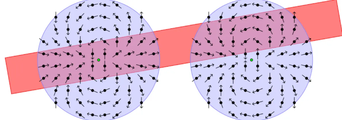
(u, v) rotates once around the origin on the phase coded discOPCD, see Figure 2. This has
the effect that points, whose phase differs by 90◦, have opposite phases (180◦difference) on
OPCD. Thus, they attenuate in the convolution (1). On the other hand, points with the same
or opposite phases have the same phase onOPCD. Thus, they amplify in the convolution (1).
For the convolution of OPCDwith the binarized image BI this has the effect, that the magnitude|Q(x, y)|is relatively large, if at (x, y) the laser line contains the center ofOPCD,
see Figure 2 (left). Otherwise, |Q(x, y)|is relatively small, see Figure 2 (right). So, after convolving BI with OPCD, the maxima of |Q| are located on the center of the laser line. However, lines with 90◦corners cannot be detected with this approach.
Figure 2 Phase coded discs with red laser line and small arrows visualizing the complex phase angles.
5.2
Non-maxima Suppression
To find sub-pixel accurate maxima in the convolution images, we adapted the approach of [5] in two ways. First, the magnitude ofQis used instead of the gradient’s magnitude. Second,
the normalL⊥ to the laser line direction Lis used instead of the gradient direction. The
direction of the laser lineL(x, y) is determined by half the phase angle ofQ(x, y) L(x, y) = 1
2Arg(Q(x, y)).
Thus,L⊥(x, y) is perpendicular toLat (x, y).
Non-maxima Suppression
3.1 Denote byBthe intersection of the line throughAin directionL⊥with the line segment
through the pixelsAi andAi+1 for a i∈ {1, . . . ,4}, see Figure 3. Analogously, C is the intersection in the opposite direction ofA. Thus, the values of|Q|atB andC are
linearly interpolated between the values atAiand Ai+1 respectivelyAi+4 andAi+5.
3.2 If there is no maximum atAcompared toB andC,Ais ignored in the result.
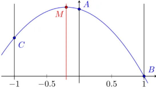
3.3 If there is a maximum atA, the sub-pixel accurate position is computed as the position
along lineL⊥ of the maximum of the quadratic interpolant of the values atA, B, and C, see Figure 4.
Thus, we store per pixel the decimal places of the sub-pixel coordinates of the maximal value and the maximal value of|Q|.
5.3
Line Tracing
The extracted line center points in BN have to be assigned to line segments. Thus, the output of Step2.5. is a list of line segments (sk)k for each image. Each line segmentsk is a list of line center points (pk,l)nj=0.k
Line Tracing
4.1 Identify start pointspi,0inBN by matching with the 3×3 pixel patterns in Figure 5 and generate a new segmentsk containing the start pointsk = (pk,0)l. Start points, which are already part of a line segment, are ignored.
L⊥ M A B C A8 A9=A1 A2 A3 A4 A5 A6 A7
Figure 3 Sub-pixel accurate position of the maximumM on line segmentCB [5].
−1 −0.5 0.5 1 M
A
B C
Figure 4 The quadratic interpolation of the values atA,B,C. AtM is the maximum of the interpolant.
4.2 For a segment sk = (pk,0, . . . , pk,l) check the 8-neighborhood of point pk,l in BN for pixels with value 1. If direct and diagonal neighbors are found, the former are preferred. If a new point pk,l+1 is found, it is appended to the corresponding line segment sk = (pk,0, . . . , pk,l+1). Visited points are tagged to avoid multiple visits in Steps4.1and4.2.
4.3 Repeat step4.2until a point is identified as end-point matching the 3×3 pixel patterns in Figure 5.
4.4 An extracted line segmentsk is ignored, if it contains less than 50 points.
6
Depth Estimation
Similar to the stereo-matching method in [4], the spatial depth of the point data is recon-structed from the disparities between images. This requires a calibrated camera system
Figure 5 Start point patterns of 3×3 pixels: The white pixels have value 0 inBN, the other
e1
e2 e3
X d1 d2 d3
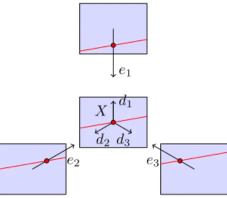
Figure 6 Schematic illustration of the four camera images with projections of epipolar linesei
of a pointX (red point) in the central camera’s image on a laser line (red line), see [4].
whose lenses are corrected. For the lens correction we use the method [6, 4] to correct all camera images to a central projection in a pre-processing step. Then, the calibration as described in Section 4 is applied.
For our camera system at every instant of time a quadruple of images is generated containing one imageIi,i= 1,2,3,4 of each camera. Accordingly, the above line extraction
algorithm yields a quadruple of e.g.Bi
N where the super-script indicates thei-th outer camera for i = 1,2,3 or the central camera fori = 4. From the line extraction step (Section 5)
we have three representations of the laser line per camera image: the line segmentssi k, the binary imageBi
N(x, y), and the sub-pixel accurate laser line center point inN
i(x, y). For each pointp4
k,lof the line segments4k of the central camera image, a depth is estimated using the images of the outer cameras:
5.1 Corresponding points in two camera images from two different cameras are identified
along epipolar lines, see Section 6.1.
5.2 For each pair of corresponding points the depth is estimated by an inverse projection,
see Section 6.2.
6.1
Epipolar Lines
After the calibration we assume that all four cameras of the camera system are co-planar and have parallel view directions. Therefore, a point ˆX at infinite depth in physical space
will have the same image coordinatesXi,i= 1,2,3,4, in all four camera imagesIi. A point ˆ
Y not at infinity with image coordinatesY4=X4 has image coordinatesYi6=Y4,i= 1,2,3, in the outer cameras. As ˆY moves closer,Yi,i= 1,2,3, moves along the negative camera
direction−di. Thus, ˆY traces out a ray in physical space pointing away from the central
camera. This line is called theepipolar lineofX4. The central projection of an epipolar line
in the outer camera images is a straight line, too. Figure 6 shows the projectionsei(X) of an
epipolar line ofX for the camera system, schematically.
For every point p4
k,l the epipolar line is computed and projected to the outer camera images. The resulting epipolar line projectionsei(p4k,l),i= 1,2,3, are rendered to imageIi using the Bresenham algorithm [1]. If during this rendering a pixel is set that is also set in
Bi
N(x, y) an intersection of the epipolar lineei with a line segment in Ii is detected. The pixel distance betweenp4k,l and the sub-pixel accurate laser line position fromNi(x, y) at
the intersection is the so-calleddisparity di(p4k,l). So, there are up to three disparities di,
To improve the quality of the reconstruction, we use subsequently the average d(p4k,l) of
the two disparities that are closest to each other. If there are less than two disparities or the two closest disparities differ too much, the computations forp4
k,l are aborted.
6.2
Inverse Projection
With the average disparity d, the depth cz in physical space ofp4k,l is estimated by
cz= wˆt 2 tan α 2 d,
whereαis the aperture angle of the camera,wthe image width in pixels, and ˆtthe camera
distance in physical space. The depthcztogether with the pixel coordinates p4k,l allow an inverse projection ofp4
k,lto 3d coordinates [cx, cy, cz]T in physical space as cx cy = 2 cz·p 4 k,l w tan α 2 =p4k,lˆt d.
7
Results
To demonstrate the effectiveness of our laser scanner system, we scanned a test scene of three wooden bricks shown in Figure 7(a). The exposure of the cameras was reduced to achieve a better contrast between the laser line and the surroundings, see Figure 7(b). During a period of five minutes, we captured ca. 210,000 points at a rate of two image-quadruples per second.
(a) (b)
Figure 7 Test scene consisting of four wooden bricks (a) and the four images of the test scene scanned with a red laser line captured by the camera system (b).
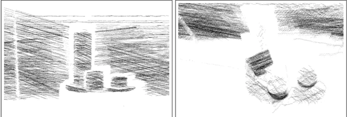
Figure 8 shows a front and a top view of the computed point cloud. The overall quality of the data allows to recognize the shapes of the different wooden bricks, especially the one in the foreground. The reconstruction has a higher quality and is more robust than the pure stereo-matching method in [4]. However, an elaborate comparison with other triangulation methods is doomed by the high costs for other hand-held triangulation devices.
Figure 8 Point cloud from two different perspectives (left: front view, right: top view) of the test scene in Figure 7 scanned with a red laser line.
The scan lines in the point clouds show some small periodic noise in view direction of the cameras. We think this might be caused by three effects:
Aliasing at the line extraction Step2.2.: The binarizationBI(x, y) in Step 2.1. creates an aliased image of the laser line. In particular, if the aliasing occurs on both sides of the line simultaneously, this may cause small steps in the detected line centers.
Intersection ofeiwith the line segments inIi in Section 6.1: The laser line position from
Ni(x, y) is at sub-pixel accuracy while the projected epipolar lineei is not. Although this approximation does not affect the disparitydi very much, a more precise intersection of the line segment withei could improve the results.
Calibration in Section 4: The laser point is not detected at sub-pixel accuracy.
Another effect that we observe in the scan data is that some of the scanned laser lines appear more than once in the data at slightly different depths. This is caused by blurry camera images, e.g. by motion blur. Additional filtering after the detection of the line centers (Section 5, Step2.2.) could be used to avoid these artefacts.
8
Conclusion and Outlook
We demonstrated in this paper how to build a laser scanner device at low costs using an existing camera system. The presented reconstruction algorithm runs on the GPU and is fast enough to compute 3D point data during the scan. Despite the remaining problems (see Section 7) the reconstruction yields better quality and is more robust than the pure
stereo-matching method in [4].
Our laser scanner is limited to scanning from a single camera position. This only allows to capture one side of an object. For complete scans of objects it is necessary to either move the camera system or rotate the object e.g. on a turn table. Combining such scans from different directions usually requires aniterative closest point algorithm.
It is possible to improve the quality of the scanned results in a post-processing step. All points on a laser line lie in the plane of the laser line fan. Thus, fitting this plane to each scan line and projecting the points onto this plane along the view direction of the cameras will probably solve most problems described in Section 7 and will be implemented soon.
References
1 J.E. Bresenham. Algorithm for computer control of a digital plotter.IBM Systems Journal,
4(1):25–30, 1965.
2 S. P. Clode, E. E. Zelniker, P. J. Kootsookos, and I. V. L. Clarkson. A phase-coded disk
approach to thick curvilinear line detection. In Proceedings of the 12th European Signal Processing Conference, pages 1147–1150, 2004.
3 K. Denker, B. Lehner, and G. Umlauf. Real-time triangulation of point streams. Engineer-ing with Computers, 27(1):67–80, 2011.
4 K. Denker and G. Umlauf. Accurate real-time multi-camera stereo-matching on the gpu
for 3d reconstruction. Journal of WSCG, 19(1-3):9–16, 2011.
5 F. Devernay. A non-maxima suppression method for edge detection with sub-pixel accuracy.
Technical Report RR-2724, INRIA, 1995.
6 F. Devernay and O. Faugeras. Straight lines have to be straight: automatic calibration and
removal of distortion from scenes of structured enviroments. Mach. Vision Appl., 13(1):14–
24, 2001.
7 G. Frankowski, M. Chen, and T. Huth. Real-time 3d shape measurement with digital stripe
projection by texas instruments micro mirror devices DMD™. Three-Dimensional Image Capture and Applications III, 3958(1):90–105, 2000.
8 Y. Furukawa and J. Ponce. Accurate, dense, and robust multi-view stereopsis. In CVPR,
pages 1–8, 2007.
9 J. Hensler, K. Denker, M. Franz, and G. Umlauf. Hybrid face recognition based on real-time
multi-camera stereo-matching. In G. Bebis et al., editors, Advances in Visual Computing,
volume 6939 ofLecture Notes in Computer Science, pages 158–167, 2011.
10 R. A. Jarvis. A laser time-of-flight range scanner for robotic vision. IEEE Trans. Pattern Anal. Mach. Intell., 5(5):505–512, 1983.
11 R. A. Jarvis. A perspective on range finding techniques for computer vision. IEEE Trans-actions on Pattern Analysis and Machine Intelligence, 5(2):122–139, 1983.
12 A. Klaus, M. Sormann, and K. Karner. Segment-based stereo matching using belief
propa-gation and a self-adapting dissimilarity measure. InProc. of the 18th Int. Conf. on Pattern Recognition, pages 15–18, 2006.
13 J. L. Posdamer and M. D. Altschuler. Surface measurement by space-encoded projected
beam systems. Computer Graphics and Image Processing, 18(1):1 – 17, 1982.
14 D. Scharstein and R. Szeliski. A taxonomy and evaluation of dense two-frame stereo
corre-spondence algorithms. Int. J. Comput. Vision, 47(1-3):7–42, 2002.
15 C. Teutsch. Model-based Analysis and Evaluation of Point Sets from Optical 3D Laser Scanners. Shaker Verlag, 2007.
16 A. Wehr and U. Lohr. Airborne laser scanning - an introduction and overview. ISPRS Journal of Photogrammetry & Remote Sensing, 54(2-3):68–82, 1999.
17 S. Winkelbach, S. Molkenstruck, and F. M. Wahl. Low-cost laser range scanner and fast
surface registration approach. InDAGM-Symposium, pages 718–728, 2006.
18 R. Yang and M. Pollefeys. A versatile stereo implementation on commodity graphics
hard-ware. Real-Time Imaging, 11(1):7–18, 2005.
19 S. Zhang and S.-T. Yau. High-resolution, real-time 3d absolute coordinate measurement