Bayesian Model Averaging. An Application to Forecast Inflation in Colombia

Bogotá Colombia Bogotá Colombia Bogotá Colombia Bogotá Colombia Bogotá Colombia Bogotá Colombia Bogotá Colombia Bogotá Colombia Bogotá

-Application to Forecast Inflation in Colombia

Por:

Eliana González

Núm. 604

2010

INFLATION IN COLOMBIA?

ELIANA GONZ ´ALEZ†

([email protected]) BANCO DE LA REP ´UBLICA

ABSTRACT. An application of Bayesian Model Averaging, BMA, is implemented to

con-struct combined forecasts for the colombian inflation for the short and medium run. A model selection algorithm is applied over a set of linear models with a large dataset of po-tential predictors using marginal as well as predictive likelihood. The forecasts obtained when using predictive likelihood outperformed the ones obtained when using marginal likelihood. BMA forecasts reduce forecasting error compared to the individual forecasts, equal weighted average, dynamic factors model and random walk forecasts for most hori-zons. Additionally, the BMA outperformed for some horizons the frequentist Information theoretic model average, ITMA, when the weights of both methodologies are build based on the predictive ability of the models.

Key words and phrases. Bayesian model averaging, forecast combination, Inflation, Infor-mation theoretical model averaging.

JEL clasification. C11, C15, C52, C53.

Date: March 2010.

?

The opinions expressed here are those of the authors and do not necessarily represent neither those of the Banco de la Rep ´ublica nor of its Board of Directors. As usual, all errors and omissions in this work are our responsibility.

†

1. INTRODUCTION

For monetary policy it is important to count with reliable forecasts for inflation in order to make appropriate decisions. This has lead to a permanent effort of econometrists in trying to find ways of reducing forecasting errors, developing and implementing differ-ent methodologies of forecasting and forecast combination. On the other hand, available information that might help to explain the dynamics of inflation and help to generate bet-ter forecasts has been widening and all this information has to be summarized in some way and be incorporated in a forecasting model. Given that the true model driving in-flation is unknown, the issue then is how within a large set of potential predictors can we find a good model or some candidate variables that explain the dynamics of inflation and help to predict it in the future?. In this regard, dealing with a large dataset, a com-monly use methodology that summarizes the information contained in all the available variables and thus reduces the dimensionality of the problem is factor models (Stock and Watson [2002], Boivin and Ng [2005], Forni et al. [2000], Forni et al. [2005], among others). With this methodology the number of possible predictors is reduced to a few ones and a model with those common factors as explanatory variables is estimated to produce fore-casts. There exist another approaches to reduce dimensionality which basically consist on selecting variables according to some criteria and shrinkage methods (See Hastie et al. [2009] for a description of some of these methods).

Another important issue that arises in forecasting is that a model that fit well the histor-ical data, not necessarily generate the most accurate forecasts for the future. One partic-ular model can be good at predicting some horizons, or can do well predicting in some situations, for instance being able to predict some future movement as a reaction to some shock and there might be another model(s) able to predict well in some other situations. Thus, in practice we cannot trust in just the forecast generated by one single ”good” model, instead we can obtain several forecasts from different specifications and method-ologies which need to be summarized in a single output. It has been found that a com-bined forecast reduces forecast error compared to a particular forecasting model (Bates and Granger [1969], Newbold and Granger [1974]). This is in part because the combined forecast may cancel out the possible biases of the individual forecasts, and it also may re-duce to some extent the misspecification of each particular model. This issue has lead to the development and widespread use of forecast combination thecniques. The standard one is the simple or equal weigthing average, but most of the methodologies of forecast combination consist on constructing weights to average individual forecasts according to some criteria based on the fit of the model (See Clemen [1989] for a review of the litera-ture on forecast combination), or more recently proposed, based on the predictive ability of each model (Eklund and Karlsson [2005], Kapetanios et al. [2006]).

Bayesian model averaging, BMA, is a procedure that allows to select models consistently from a model space, without having to analyse every particular model in order to de-termine which ones better fit the data or help to predict more accurately a variable of interest. This can be done by drawing a sample of models from the distribution of the model space and rank them according to the posterior probability, which depends on the

likelihood of the model and a prior belief on each particular model. Thus, the weight assigned to each forecast to be combined is given by the posterior probability of each model. The pioners in using this approach to forecast combination are Raftery et al. [1997] and many applications have been developed to forecast inflation, such as the works of Wright [2003], Jacobson and Karlsson [2002], Koop and Potter [2003], Eklund and Karls-son [2005], Kapetanios et al. [2006] and Kapetanios et al. [2008] among others, showing good performance of BMA compared to other combined forecasts.

In this paper an application of BMA to forecast Colombian inflation is performed, consid-ering a large dataset of variables related to real economic activity, monetary, credit and exchange rate variables and prices. Both, marginal and predictive likelihood are used in order to construct the posterior probabilities to select first the best predictors and then the models to be combined. The predictive likelihood has the advantage over the marginal likelihood that it considers the performance of the model out of sample and thus deals with the issue that not necessarily a good in-sample model is a good predictor of the future. Additionaly, an empirical comparison of the performance of the BMA forecasts to other combined forecasts such as the simple average, an average based on an infor-mation criteria, known as Inforinfor-mation theoretical model averaging,ITMA forecast, and the random walk forecast is done. The results support the findings of other authors, that combined forecasts performs better than the individual forecasts. The combined fore-casts whose weights are build based on the predictive ability of each individual model significantly reduces the forecasting error compared to those combined forecasts whose weights are build based on the in-sample fit of each model. All the combined forecasts performed better than the random walk. Comparing BMA and ITMA, both based on the predictive ability of the models, the results favor BMA for some horizons, however for other horizons ITMA performs better.

The remainder of the paper is structured as follows. Section 2 describes the Bayesian model averaging methodology and particularly when is used for forecast combination. In section 3 the implementation of this methodology to forecast inflation in Colombia is described. Section 4 shows the results of the BMA empirical exercise for Colombian infla-tion as well as the evaluainfla-tion of the obtained forecasts comparing to forecasts generated by different approaches. Section 5 concludes.

2. BAYESIANMODELAVERAGING

Bayesian Model Averaging was first thought as a model selection process, implemented by Hoeting et al. [1999], based on model uncertainty, since in practice the data generating process is unknown. It esentially works as follows: Given a set ofMmodelsM1, . . . ,MM, for which the researcher has a prior belief about the probability of Mi being the true model,P(Mi)fori= 1, . . . , M, using Bayes theorem and the observed data,Y, the pos-terior probability that each model is the true one is given by:

P(Mi/Y) = m(Y/Mi)P(Mi) M P i=1 m(Y/Mi)P(Mi) (2.1)

wherem(Y/Mi)is the marginal likelihood of modelidefined as

m(Y/Mi) = Z

L(Y/Θi,Mi)P(Θi/Mi)dΘi (2.2) whereLis the likelihood and P(Θi/Mi)istheposteriordensityof theparametervectorof modeli. For any quantity of interest,∆, which may be a parameter, or a function of some param-eters, its posterior distribution can be obtained as the weighted average of the posterior distributions under each model in the set of available models. The weights correspond to the posterior model probabilities.

P(∆/Y) =

M X

i=1

P(∆/Y,Mi)P(Mi/Y) (2.3)

Following the same spirit, for a functiong(∆), its posterior distribution is given by: E(g(∆)/Y) =

M X

i=1

E(g(∆)/Y,Mi)P(Mi/Y) (2.4)

In particular, for the conditional forecast,Y˜t+h=E(Yt+h/Yt), the optimal forecast combi-nation is obtained as the weighted average of the forecast generated by each model.

E(Yt+h/Yt) = M X

i=1

E(Yt+h/Yt,Mi)P(Mi/Y) (2.5)

When considering the case of variable selection, the posterior probability that variablej is included in the true model is given by

p(Xj/Y) =

M X

i=1

I(Xj ∈Mi)P(Mi/Y) (2.6)

whereI(Xj ∈ Mi)is an indicator variable, taking value of one when variable Xj is in modelMiand zero otherwise.

In order to implement this in practice, the researcher only has to define the prior prob-ability of each model,P(Mi), and the prior distribution of the parameter vector in each model,P(Θi/Mi). On the other hand, the models not necessarily have to be linear One important issue when implementing this methodology for variable or model selec-tion, as well as, for forecast combination is the number of available models considered.

When the set of models is very large, sometimes the calculation of the posterior prob-ability for each particular model is something impractical. Madigan and Raftery [1994] suggested using some algorithm to reduce the model space in such a way that only those models with non negligible posterior probability are considered.

In practice, accounting for model uncertainty, the idea is to find a set ofM ”good” mod-els from a large set of possible predictors. Thus, if we have, sayK predictors, the model space contains2K possible models. We can restrict the model space considering only those models containing up to k predictors, k < K, so that the model space reduces to( k P j=0 K j

)possible models, considering also the model with an intercept only. As the number of possible models is still huge, the calculation of the posterior probability for each particular model is burdensome. Jacobson and Karlsson [2002] suggested employ-ing MCMC algorithms to visit a signficative sample of the full model space and calculate for those visited models the posterior probability. Since the MCMC takes draws from re-gions where posterior probabilities are high, then we will be able to choose models with a non-negligible posterior probability.

In particular, the reversible jump algorithm, RJMCMC proposed by Green [1995], seems to be a convenient method to deal with this issue. The algorithm works as follows: From an initial state of the chain,(θM,M), whereM indicates teh model andθM the pa-rameters of dimensiondim(θ_M)

• Propose a jump from modelMto modelM∗ with probabilityj(M/M∗) • Generate a vectorufrom a proposal densityq(u/M,M∗)

• Set(θ_M∗, u∗) = g_M,M∗(θ_M, u), where gis a specified invertible function andu, u∗

satisfydim(u) +dim(θM) =dim(u∗) +dim(θM∗)

• Accept the move with probability α= min 1,L(Y/ΘM∗,M ∗_)P(Θ M∗/M∗)P(M∗)j(M/M∗)q(u∗/Θ_M∗,M∗,M) L(Y/Θ_M,M)P(Θ_M/M)P(M)j(M∗/M)q(u/Θ_M,M,M∗) × ∂gM,M∗(θ_M, u) ∂(θM, u) (2.7) and setM =M∗if the move is accepted.

Following the works of Jacobson and Karlsson [2002] and Eklund and Karlsson [2005], the algorithm simplifies enormously by only considering the following local moves: add or drop a variable and swap one variable at a time.

(1) For the add or drop jump, one selects a variable from the whole dataset at random and check if it is already in the current model. Drop it if it is in the model or add it if it is not in the model. The probability of this move isj(M/M∗) = j(M∗/M) =

1

K, withKthe number of available variables.

(2) For the swap jump, one selects a variable in the model at random and swap it for a randomly selected variable outside the model. The probability of this move is

j(M/M∗) =j(M∗/M) = _k(K1_−k), withkthe number of variables in the model.

If in addition all parameters of the proposed model are generated from a proposal distri-bution, then

• (θM∗, u∗) = (u, θ_M)withdim(θ_M) =dim(u∗)anddim(θ_M∗) =dim(u)

• the Jacobian

∂g_M,M∗(θM, u) ∂(θM, u)

= 1 (2.8)

Additionally, if considering the posterior distribution ofθM,P(θM/Y, M)as the proposal distribution for the parameters space, then

The acceptance probability of the move fromM toM∗simplifies further to

α= min 1,L(Y/Θi,M ∗_)P(Θi/M∗_)P(M∗₎ L(Y/Θi,M)P(Θi/M)P(M) (2.9) or α = min 1,m(Y/M ∗_)P( M∗) m(Y/M)P(M) (2.10) 2.1. The priors.

2.1.1. The prior model distribution. In the literature, different kind of prior for the probabil-ity that each model is the true one have been set. The most commonly used is assuming that all available models have the same odd of being the true model, that isP(Mi) = _M1 fori= 1, . . . , M, which is known as a non-informative prior. Another, useful informative prior on the models is given by (Eklund and Karlsson [2005]):

P(Mi)∝δki(1−δ)k−ki (2.11)

wherek is the maximum number of variables allowed in a model,ki is the number of variables included in modeliandδ is set such that the expected model size is equal to some prior. In particular, whenδ = 0.5the prior model probability is the same for each model.

2.1.2. The prior distribution for the parameters. Considering linear regression models of the formY =Zγ+, whereγ = (α, β0)0,Z = (1, X)contains the explanatory variables and ∼N(0, σ2I)

An alternative for prior distribution of the variance of the error term is the Jeffrey0s non-informative prior

p(σ2)∝ 1

σ2

(2.12) The prior distribution for the vector parameterγ/σ2 is the g-prior distribution, (Zellner [1986]) p(γ/σ2,M)∼Nk+1(0, cσ2(Z 0 Z)−1) (2.13) with c= K2 _{ifT ≤K}2 T ifT > K2 (2.14)

as suggested by Fernandez et al. [2001]

These set of priors lead to the posterior on the parameters

p(γ/Y)∼tk+1(γ1, S1, M1, υ1) (2.15) whereγ1 = _c+1c ˆγandˆγis the OLS estimate,

S1= c c+ 1(Y −Zγˆ) 0 (Y −Zˆγ) + 1 c+ 1Y 0 Y (2.16) M1 = c+ 1 c Z 0_Z (2.17) This leads to the marginal likelihood, which is also a multivariate t-distribution

m(Y/M)∝(c+ 1)−(k+1)/2S₁(−T /2) (2.18)

2.2. The predictive likelihood. A way to avoid the in-sample overfitting problem, which may appear when using marginal likelihood, is to consider the predictive ability of the models instead of the in-sample fit to construct the weights of the models to be average. In order to achieve this, the full sample (y₁,· · ·,y_T) is split into two parts: Y∗ andY˜ with T1 andT2 observations, respectively, where the first part of the sample is used to obtain the posterior distribution on the parameters and the second part is used to eval-uate the model performance. The size of the training and out-sample parts are chosen in such a way that with the minimal training subset,Y∗, a proper posterior distribution, P(Θi/Y∗,Mi), is obtained and Y˜ is the complement set of observations. As the out-sample size increases, the predictive likelihood will be more stable and should perform better, Berger and Pericchi [1996].

YT×1= Y_T∗_1×1 ˜ YT2×1 (2.19) Thus, the posterior predictive likelihoodP( ˜Y /Y∗,Mi)conditional onY∗and the model Miis given by

P( ˜Y /Y∗,Mi) = Z

L( ˜Y /Θi, Y∗,Mi)P(Θi/Y∗,Mi)dΘi (2.20) whereLis the likelihood andP(Θi/Y∗,Mi)is the posterior distribution on the param-eters of model i. The predictive density gives the distribution of future observations

(y_T1+1,· · · ,y_T) conditional on the observed sampleY∗. A large value ofP( ˜Y /Y∗,Mi) indicates a good predictive model.

Under the set of priors above, the predictive density ofY˜ = (y_T1+1,· · · ,y_T)is P( ˜Y /Z, Z˜ ∗, Y∗, γ∗, σ2)∼NT2( ˜Zγ

∗

, σ2IT2) (2.21)

whereZ˜is the out-sample matrix of explanatory variables andγ∗are the parameter vec-tor estimated with the training sample. Then, the predictive posterior density ofY˜ is a multivariate student distribution.

˜ Y /Z, Z˜ ∗, Y∗∼tT2( ˜Zγ1, S ∗_,(I T2 + ˜Z(M ∗₎−1_Z˜0₎−1_{, T} 1) (2.22)

with density function P( ˜Y /Z, Z˜ ∗, Y∗)∝ S ∗T1/2_|M∗_|1/2 M ∗_{+ ˜Z}0_Z˜ 1/2 ×[S ∗ + ( ˜Y −Zγ˜ 1)0(IT2 + ˜Z(M ∗ )−1Z˜)−1( ˜Y −Zγ˜ 1)]−T /2 (2.23) whereS∗,γ1 andM∗ are defined the same asS1,γ1 andM1for the marginal likelihood but calculated over the training sample only.

Having the predictive likelihood, the posterior probability or the weight asigned to each model is obtained by replacing the marginal likelihood with the predictive likelihood,

P(Mi/Y , Y˜ ∗) = P( ˜Y /Y∗,Mi)P(Mi) M P i=1 P( ˜Y /Y∗,Mi)P(Mi) (2.24) 3. EMPIRICALAPPLICATION

3.1. Data. The dataset used for the empirical application consists on 73 monthly macroe-conomic Colombian time series from 1999:11 to 2009:12. This sample was chosen given

the availability of all series and to avoid a structural change observed in several macroe-conomic variables during 1998 as shown in Melo and Nu ˜nez [2004] among others. The data are grouped into three categories: Real Activity (26 series), Prices (23 series), Credit, Money and Exchange Rate (24 series)1.

The series are seasonally adjusted using Tramo-Seats methodology proposed by Caporello and Maravall [2004], then the variables are transformed as annual growth rates or twelve-month log differences, except the ones that are measured as balances or are already mea-sured as growth rates. Inflation is meamea-sured as the twelve-month growth rate and it is also included in the set of predictors. Thus, the sample used to implement the methodol-ogy of BMA is from 1999:11 to 2007:12 leaving the last two years to generate recursively out-sample forecasts and evaluate the forecasting performance.

3.2. Implementation. As the purpose of the empirical exercise is to get forecasts for in-flation for one to twelve months ahead, the following procedure is performed for each horizon, since the models considered are univariate linear models of the form Yt+h = α+

k P j=1

Zj,t−iγj +t+h, where the dependant variable is observed int+hrather than t in order to construct direct forecasts that do not require forecasting the predictors. The explanatory variables are observed at timetor with some lagt−iand the model may include up tokpredictors.

Two exercises of BMA are performed. In the first one, the marginal likelihood is used to calculate the posterior probabilities of variables and models using the sample from 1999:11 to 2007:12. In the second exercise, the predictive likelihood is used. In order to calculate the posterior probabilities of the variables and models for the later exercise, the sample is split asY∗ =

n

y_{N ov/1999},· · ·,y_Dec/2004o as the training sample andY˜ =

n

y_{J an/2005},· · · ,y_Dec/2007oas the hold-out sample.

The procedure consists of two stages. In the first stage a pre-selection of variables is done in order to reduce the dimensionality of the problem, so that only variables with significant predictive power are included in the data set. Given the dimension of the model space, 273 possible models, it is initially restricted to those models with up to five explanatory variables entering with timet, i.e. no lags are considered. So, Yt+h = α+

5

P j=0

Zj,tγj+t+h. Thus, the number of possible models is reduced to about 5 P j=0 73 j ≈ 16 million. δ in (2.11) is set as0.065, so that the prior expected model size is 5 variables. The size and the variables included into the initial model are chosen at random to start the chain. The Markov chain is run 7 million steps and the algorithm calculates the pos-terior probability of each variable being included into a model. The first 2 million draws are leaving out as burn in sample, so that, they are not considered for the calculations

of posterior probabilities. The 20 variables with the highest posterior probability are se-lected to construct the data set for the second stage of the process. If total CPI inflation is not selected, it is forced to enter in the new dataset.

In the second stage, two lags of each of the pre-selected variables are added to the dataset. Thus, a total of 60 variables are considered as predictors. As the number of possible mod-els is huge,260_{, the model space is restricted to those models with up to 8 explanatory} variables. This timeδ = 0.13 is set for a prior expected model size of 8 variables. With that restriction, the model space consists of

8 P j=0 60 j

≈3000 million models approximately. Thus, the models are of the formYt+h=γ0+

8

P j=0

Zj,t−iγj+t+h, whereicould be0,1, or,2. Again, the size and variables of the initial model are randomly chosen to determine the initial state of the chain. This time a sample of 11 million models is drawn and the ini-tial 1 million draws are excluded as burn−in sample. With the accepted models in the remaining draws, the algorithm calculates the posterior probability of each model and the 20 models with higher posterior probabilities are selected to generate the combined forecasts.

With the selected models, recursive out of sample forecasts are obtained for each hori-zon, in the sample 2008:01-2009:12, for a total of 24 out-sample forecasts. The BMA forecasts are obtained as the weighted average of the forecast of the 20 selected mod-els. The weights are given by the posterior probability of each model, re-weighted so that they sum to unity. The weigths change over the forecasting sample. They are calculated for each out-sample period with information up to the previous forecasting period. That is, when using predictive likelihood, the training sample is alwaysY∗ =

n

y_{N ov/1999},· · ·,y_Dec/2004oand the hold-out sample changes for each forecasting period

˜

Y = ny_{J an/2005},· · · ,y_Dec/2007+j−1

o

, j = 1,· · ·,24. When using marginal likelihood,

the weigths are based on the fit of each model estimated with information up to the pre-vious forecasting period.

In order to compare the performance of the BMA forecasts, two other combined forecasts are obtained with the same set of models. The simple average forecast and the informa-tion theoretical model average, ITMA, where the weights are calculated using the AIC criteria with the forecasting errors observed up to the previous out-sample period, as suggested by Kapetanios et al. [2008]. These authors have already compared the perfor-mance of the BMA and ITMA combination to forecast inflation in the UK, however their comparison was not fair enough in the sense that the weights of BMA were obtained using the marginal rather than predictive likelihood, while the ITMA combination uses the predictive performance of the models to calculate the weights, bringing support for the later. In order to make the comparison between BMA and ITMA fairer, an additional

exercise of information theoretical model average, ITMA, is also performed, where the 20 models to be average are selected as the ones with smaller AIC criterium over the hold-out sample.

A final forecasting exercise based on a dynamic factors model using the same database and for the same sample period is carried out in order to compare the forecasts generated by this well known alternative of forecasting with many predictors with those generated by BMA. See Gonz´alez et al. [2009] for details of the dynamic factors model estimated for the Colombian inflation.

On the other hand, two additional exercises are performed to check selection model con-sistency. The first one consists on running the algorithm with the same information and samples but starting the chain in a different state. The aim of this exercise is to check whether the initial state of the chain influences the results of selected variables and mod-els, even though some portion of the draws are leaving out as burn-in sample. This ex-ercise has already been performed by Eklund and Karlsson [2005] with simulated data, founding that no matter the initial state of the chain always the true model is selected. The second exercise pretends to check consistency over time, as a maner of determining whether the forces driving inflation have changed, especially in the last two years of the sample where an important decline in inflation has been observed (See Figure 3.1). The later exercise consists on taking the full sample and run the algorithm of variables and model selection. i.e. using the sample from 1999:11 to 2009:12 for the marginal likeli-hood and the augmented hold-out sample Y˜ = ny_{J an/2005},· · · ,y_Dec/2009oto calculate the predictive likelihood and compare variables and selected models with the ones ob-tained with the sample until Dec/2007 to check if they have changed or remained the same. This run of the algorithm is done using the same initial state of the chain as the first selection exercise in order to control at least one source of variation of the results.

4. EMPIRICALRESULTS

In this section the main results obtained from the empirical application of BMA to forecast colombian inflation are presented.

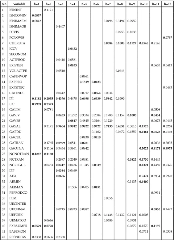
Tables A.18 and A.19 show the variables with higher posterior probability of being a ex-planatory variable for each horizon based on predictive and marginal likelihood respec-tively. It can be seen that the best predictors for inflation changes with the horizon and they also differ according to which likelihood, marginal or predictive, is used to calculate the posterior probabilities.

When considering predictive likelihood, past information of total CPI inflation is one of the variables that help the most to predict inflationhperiods ahead, as it was expected, mainly for short run horizons (1 to 2 months). There is a wide variety of variables that seem to be good predictors for inflation, including some components of CPI inflation as well as producer prices and its components. In particular, for the short run, variables like inflation of some components of the CPI such as health, tradables and non tradables, net international reserves and the industrial production index seem to be important to predict inflation. For the medium run, in addition to those variables, expectations about production, lending interest rate, nominal exchange rate and several components of CPI inflation are among the variables with higher predictive power. Finally, the inflation of other goods and services and administrated goods, the same as the producer prices of agriculture and final consumption goods are among the set of best predictors in the long-run (10,11,12 months). On the other hand, when considering the marginal likelihood, the set of variables is wider and mixed. It is worth mentioning that variables such as interest rate, exchange rate and expectations about economic activity and prices, which seem to be important to predict inflation for several horizons.

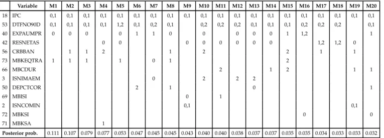
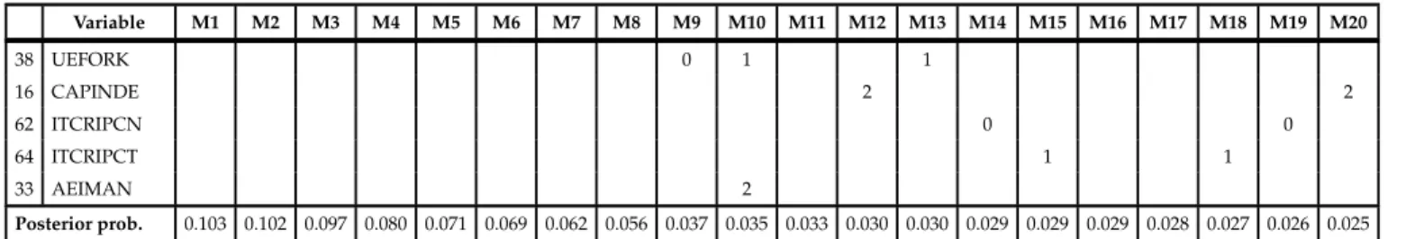
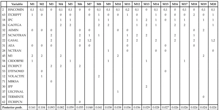
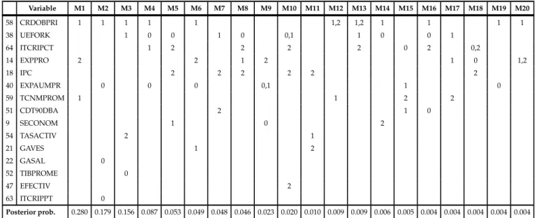
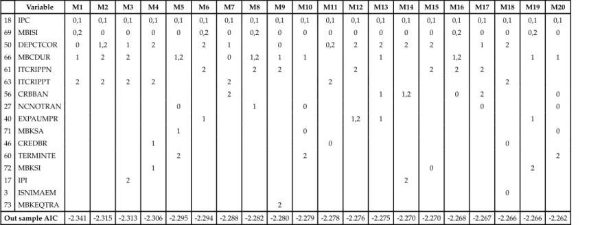
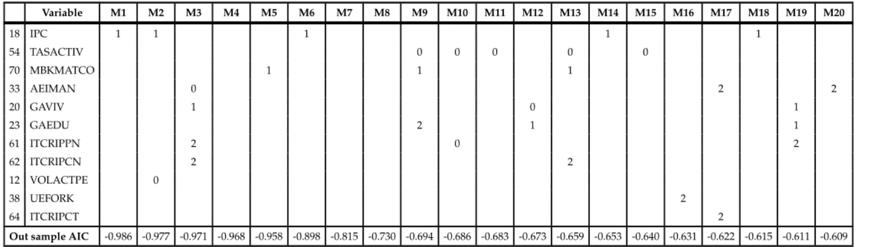
Tables A.20, A.21, A.22 show the 20 models with the top higher posterior probability for horizons 1,6 and 12 months respectively, according to the predictive likelihood2. For each horizon, the selected models share most variables, they differ one another in only a few variables or in the lags with which the variables enter in the model. The variables included in the models are not always the ones with higher posterior inclusion probabil-ities in the first step of the algotithm. The average model size is seven variables. Similar results are obtained when using marginal likelihood and the ITMA criteria. Tables A.23, A.24, A.25 show the 20 models with the top higher posterior probability for horizons 1,6 and 12 months respectively, according to the marginal likelihood and Tables A.26, A.27, A.28 show the 20 models with the smaller AIC criteria as defined in Kapetanios et al. [2008]. Comparing the set of selected models by the three criteria it can seen that the selected models have some variables in common for each horizon, especially between BMA based on predictive likelihood and ITMA criteria, what is not surprising since both methodologies use as selection criteria a measure of the predictive ability of the models.

On the other hand, when a second run of the algorithm of selection of variables and mod-els starting the chain from a different state was performed, the results slightly change. It was found that more than 70%of the variables and models selected in the fisrt run are still selected in the second run 3. Moreover, most of the variables not selected by the second run of the algorithm have a small posterior inclusion probability in the first run, which may not affect drastically the results of models selecction.

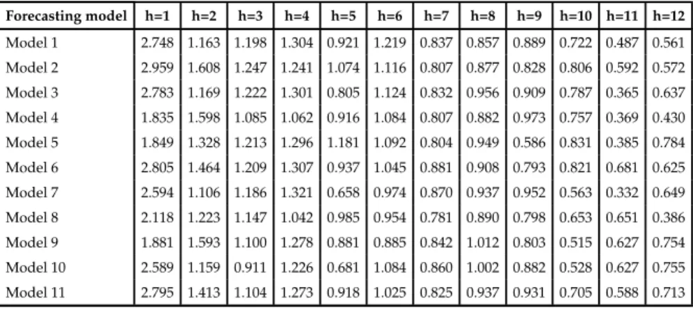
Using the different combination methodologies described above, pseudo out-sample fore-casts are generated for 24 periods starting in 2008:01. They are indeed psuedo out-sample and not real out-sample, since most of the information related to real activity is available with some lag (around four months) and some variables are subjected to reviews. The information in the dataset is the one available at Dec/2009. Tables 5.12, 5.13, 5.14 show the evaluation of the individual forecasts as well as the combined forecasts obatined for each of the three methodologies, BMA based on predictive and marginal likelihood and ITMA, respectively. It shows the RMSE of each forecast relative to the RMSE of the ran-dom walk forecast. The main results can be summarized as follows. For most horizons, the BMA forecasts based on predictive likelihood outperforms every individual forecasts, while the BMA forecast based on marginal likelihood does not outperformed some of the individual forecast for the horizons considered. Similar results are obtained for the ITMA forecast. On the other hand, the BMA based on predictive likelihood reduces sig-nificantly the forecasting error compared to the BMA based on marginal likelihood for some horizons. The BMA outperforms the simple average and the ITMA forecast for all horizons when considered the models selected by the ITMA methodology, however when selecting the models by BMA using predictive likelihood, the ITMA combination performs better for some horizons. The ITMA forecast evaluation are quite similar to the simple average because the assigned weights are almost equal for all models, producing similar forecasts to the simple average. Additionally it was found that the BMA produces more accurate forecasts than the dynamic factors model for horizons further than three months.

Although the RMSE seems to increase with the horizon, in average the smaller RMSE is for the ITMA2 combination, followed by BMA-pl, BMA−ml, simple average and dy-namic factor model. See Table 5.15 for detailed results. The numbers in italic and bold make reference to the combinations which significantly reduce the RMSE relative to the random walk forecast according to the modified Diebold and Mariano Test, MDM, for equal forecast accuracy, (Harvey et al. [1998])4. It is worth noticing the important reduc-tion in the forecasting error relative to the random walk. The further the horizon, the more significant the reduction in RMSE of the BMA and ITMA relative to the random walk. The RMSE of the random walk forecast is more than twice the RMSE of the BMA

3_{Results of all variables and the posterior inclusion probabilities for the second run are available under} request

4_{Due to the small out−sample to evaluate the combinations, the results of the MDM test have to be} taken cautiously and in order to support these results, a bootstrapping approach was used to compare the predictive ability of the combinations. See Gonz´alez and Reyes [2009] for details.

and ITMA for the further horizons. This is confirmed by the results in Table 5.16, since for both, BMA-pl and ITMA2 forecasts, more than 90%of the bootstrapping samples of forecasting errors, present for most horizons a reduction of more than5%in the RMSE relative to the random walk forecast. Another important result is that although the more sophisticated forecasts combination (BMA and ITMA) performed well, the simple aver-age also produces good forecasts, which is due basically to the appropriate selection of models by BMA or ITMA algorithms. Thus, those algorithms are useful to select models with high predictive power, which may suggest considering some of the individual fore-casting models as alternatives to obtain good forecasts for inflation by themselves and not only as an intermediate step to get an appropriate combination of forecasts.

On the other hand, for the final exercise of running the algorithm of selection of vari-ables and models with the full sample 1999:11 to 2009:12, it was found that on average 40%of the variables with higher posterior probability are still selected with the whole sample when using predictive likelihood. However, some of the variables with higher inclusion probabilities are not longer selected and instead some new variables appear to have higher predictive power. It is worth mentioning that variables such as the producer prices of mining products, which includes oil prices and producer prices of agriculture, M2, real exchange rate and prices of imported goods seem to have an important predic-tive power with the sample until Dec/2009. On the other hand, the results do not change much when using marginal likelihood, since on average 70% of the variables are still selected with the full sample. It means that adding two more years of information, the in−sample fit is not affected severely. However, the predictive ability of some variables to forecast inflation have changed to some extend during the last two years. In Table A.18, the numbers in italic and bold indicate the variables which are selected by running the algorithm with the whole sample using predictive likelihood and Table A.19 shows in bold and italic the variables which are not longer selected with the full sample when using marginal likelihood.5.

5. CONCLUDING REMARKS

In this work an alternative approach of forecasting based on a large dataset of potential predictors is implemented for the Colombian inflation. Bayesian model averaging is a useful and consistent way to select variables and models with high predictive power. The variables chosen as best predictors for inflation have not change significantly over the last two years, especially for the short run, however for further horizons, it seems that the forces driving inflation have change over time. On the other hand, the variables chosen as good predictors differ whether they are selected using marginal or predictive likelihood, what suggests, one more time, that not all models with good in-sample fit are good at forecasting.

5_{Results of the posterior inclusion probabilities of all variables and selected models for the run of the} algorithm with the whole sample are found in the Appendix at the end of the document

It was found that the BMA technique outperforms the random walk forecast as well as the simple average combination and is a good competitor of other frequentist forecast combination thecniques, such as the information theoretical model averaging, ITMA. A gain of using BMA in reducing the forecasting error is observed as the horizon increases, what is very helpful for our purpose of forecasting inflation in the medium term. The forecast combinations whose weigths are based on the predictive ability of the models to be average reduces the forecasting error relative to combinations whose weights are based on the fit of the model.

On the other hand, in this application it was found that BMA based on predictive like-lihood is for some horizons better than ITMA when the combination is made over the models selected by BMA, however when the selection of models is made by the ITMA criteria, the combined forecast obtained by the BMA weights performs better for all con-sidered horizons.

For future research, some issues arise regarding the BMA methodology. In first place, how often the selection of variables and models should be done in order to continue applying this methodology on a regular basis, given that the results are influenced by the sample, specially when using the predictive likelihood. A second concern is about the priors and the algorithm used to select the variables and models, having into account the findings of Ohara and Sillampaa [2009], that the performance of the method depends on the priors and how it is implemented. A third issue is regarding the number of models to be averaged.

A final question that arises from this work is regarding the transformation used for the response variable and the predictors. Would it make a crucial difference in the results whether the variables are measured as first or second differences to guarantee stationarity of all variables involved in the analysis?.

Table 5.1: Variables with high posterior probability - Predictive Likelihood No Variable h=1 h=2 h=3 h=4 h=5 h=6 h=7 h=8 h=9 h=10 h=11 h=12 1 ISRSINT 0.1121 2 ISNCOMIN 0.0837 3 ISNIMAEM 0.0842 0.0496 0.3194 0.0959 4 ISNIMAOB 0.4407 5 PCVIS 0.0953 0.1033 6 PCNOVIS 0.0797 7 CHBRUTA 0.0684 0.1008 0.1527 0.2546 0.2146 8 ICCV 0.0452 9 SECONOM 10 ACTPROD 0.0418 0.0581 11 EXISTEN 0.0853 0.0655 0.0413 12 VOLACTPE 0.0510 0.0713 13 CAPINVOP 0.0461 14 EXPPRO 0.1519 0.0423 15 EXPSITEC 0.0495 16 CAPINDE 0.0442 0.0917 0.0664 0.0634 17 IPI 0.1182 0.2035 0.4376 0.4478 0.6498 0.6939 0.5842 0.1090 18 IPC 0.9989 0.7373 19 GALIM 0.0781 0.0506 20 GAVIV 0.0453 0.1272 0.3534 0.2584 0.1788 0.1157 0.1005 0.0434 21 GAVES 0.0817 0.4845 0.3164 0.1229 0.0673 0.0445 22 GASAL 0.3171 0.9604 0.9812 0.9922 0.9722 0.7435 0.4652 0.3016 0.1525 0.0258 23 GAEDU 0.1102 0.0672 0.1559 0.1461 0.0528 0.0198 24 GACUL 0.0438 0.0418 25 GATRAN 0.1765 0.0979 0.0541 0.0781 0.2036 0.3035 26 GAOTGA 0.1106 0.5464 0.5661 0.0942 0.3025 0.8171 0.9975 27 NCNOTRAN 0.1267 0.1160 28 NCTRAN 0.2897 0.2349 0.0481 0.0822 0.1730 0.1445 29 NCREGUL 0.0483 0.0417 0.0436 0.1045 0.0539 0.1321 0.4489 0.7376 30 IPP 0.0384 0.0469 31 AEA 0.0686 0.2474 0.6934 0.9920 32 AEMIN 0.1135 0.1400 33 AEIMAN 0.1506 0.0705 0.0451 34 PBPRODCO 0.0911 35 PBM 0.0556 36 UECINTER 37 UECFINAL 0.0715 0.0923 0.0882 0.0830 0.2497 38 UEFORK 0.0718 0.1435 0.1432 0.1121 0.1005 39 UEMATCO 0.0646 0.0586 0.0931 40 EXPAUMPR 0.0529 0.0778 0.0879 0.1570 0.1197 41 BASEMON 0.0711 0.0308 42 RESNETAS 0.3338 0.5606 0.2368 (continued ...)

(continued ...) No Variable h=1 h=2 h=3 h=4 h=5 h=6 h=7 h=8 h=9 h=10 h=11 h=12 43 M1 0.0554 0.0384 0.0843 44 M2 45 M3 0.0346 46 CREDBR 0.0524 0.0407 0.0811 0.2295 0.2854 0.0611 47 EFECTIV 0.1494 0.1517 0.1106 0.0540 48 TOTALDEP 49 DEPCTAHO 0.0490 0.1154 0.1172 0.0250 50 DEPCTCOR 0.0695 0.0656 0.1158 51 CDT90DBA 0.0588 0.0801 0.0910 0.1515 0.2467 0.2123 0.1062 0.0439 52 TIBPROME 0.0617 0.0540 0.0822 0.2882 0.2251 0.0621 0.0782 53 DTFNO90D 0.0914 0.0617 54 TASACTIV 0.0974 0.0840 0.1168 0.1147 0.0981 0.0767 55 CRBTES 0.0341 56 CRBBAN 0.0542 57 CRBCORP 58 CRDOBPRI 0.0930 0.3247 59 TCNMPROM 0.2250 0.4990 0.5193 0.4627 0.2818 60 TERMINTE 0.1490 0.0998 0.0957 0.3054 61 ITCRIPPN 0.0626 0.0475 0.1427 0.2274 0.1456 62 ITCRIPCN 0.0571 0.0614 0.0506 63 ITCRIPPT 0.0576 0.1187 0.0964 64 ITCRIPCT 0.1018 0.1307 0.0754 0.0669 65 MBCNODU 0.0509 0.0688 0.1112 0.0512 66 MBCDUR 0.0877 0.0533 67 MBICOMLU 0.0835 0.0941 0.1373 0.0269 68 MBISA 0.0493 0.0449 0.0406 69 MBISI 0.1458 0.0991 0.0741 0.1645 0.1974 0.1126 0.0916 70 MBKMATCO 0.0470 0.1611 71 MBKSA 0.0665 72 MBKSI 0.0611 73 MBKEQTRA 0.0551 0.0705 0.0605 0.0787

* Posterior inclusion probabilities for the 20 variables selected for each horizon

Numbers in italic and bold indicate the variable is selected with the sample up to Dec/2009.

Table 5.2: Variables with high posterior probability - Marginal Likelihood No Variable h=1 h=2 h=3 h=4 h=5 h=6 h=7 h=8 h=9 h=10 h=11 h=12 1 ISRSINT 0.0311 0.0617 2 ISNCOMIN 0.9839 0.0568 0.0032 3 ISNIMAEM 0.0786 0.0297 0.0963 0.0268 4 ISNIMAOB 0.0909 0.9065 1.0000 0.9106 0.9978 5 PCVIS 6 PCNOVIS 0.0576 0.0252 (continued ...)

(continued ...) No Variable h=1 h=2 h=3 h=4 h=5 h=6 h=7 h=8 h=9 h=10 h=11 h=12 7 CHBRUTA 0.1939 8 ICCV 0.4736 0.4060 9 SECONOM 0.3469 0.1211 0.0048 0.0162 10 ACTPROD 11 EXISTEN 0.0001 0.0190 0.0294 12 VOLACTPE 0.5059 0.2242 0.4909 0.0121 0.0222 13 CAPINVOP 0.0576 14 EXPPRO 0.0252 0.0162 15 EXPSITEC 0.8174 16 CAPINDE 17 IPI 18 IPC 0.9416 0.2301 19 GALIM 0.2809 0.7388 20 GAVIV 0.3858 0.5701 0.9572 0.1343 0.0000 21 GAVES 0.0700 0.0290 0.0678 0.0187 0.0016 22 GASAL 0.4067 0.3424 0.0118 0.0834 0.0263 23 GAEDU 0.0319 24 GACUL 0.1336 0.0131 25 GATRAN 0.5591 0.0280 0.0456 0.0070 0.0000 26 GAOTGA 0.0144 0.9113 0.6916 0.0189 0.0985 0.0050 0.0146 0.9999 27 NCNOTRAN 0.0846 0.0682 28 NCTRAN 0.4963 0.0649 0.7279 0.9877 0.3308 0.0000 29 NCREGUL 0.5562 0.0257 0.0218 30 IPP 0.1328 0.1077 0.7718 0.7860 0.0002 31 AEA 0.0418 0.1377 0.0171 0.0035 32 AEMIN 0.0274 0.0762 0.2051 0.0223 0.0578 0.0001 0.0036 0.0376 33 AEIMAN 0.0295 0.0340 0.0086 0.0699 34 PBPRODCO 0.0644 0.1776 0.0079 0.1292 0.0589 0.0909 0.9628 0.0656 35 PBM 0.0181 0.8997 0.0634 0.0287 0.0273 36 UECINTER 0.2541 0.0660 0.9323 0.0480 0.9138 0.9998 37 UECFINAL 0.1424 0.0354 0.0528 38 UEFORK 0.0083 0.0592 0.0756 0.5999 0.0000 39 UEMATCO 0.0823 0.0254 0.0001 0.0042 40 EXPAUMPR 0.9080 0.3370 41 BASEMON 0.0677 42 RESNETAS 0.0221 0.0404 0.0168 43 M1 0.0301 0.1971 0.5095 0.0000 44 M2 0.2578 0.0000 45 M3 0.0276 0.0146 0.5631 0.0655 46 CREDBR 0.0836 0.2740 47 EFECTIV 0.0301 0.0755 0.0285 0.8285 1.0000 0.8352 0.0037 48 TOTALDEP 0.5645 0.0004 49 DEPCTAHO 0.0968 0.0047 50 DEPCTCOR 0.0134 0.0188 (continued ...)

(continued ...) No Variable h=1 h=2 h=3 h=4 h=5 h=6 h=7 h=8 h=9 h=10 h=11 h=12 51 CDT90DBA 0.5271 0.4067 0.1788 0.0666 0.0500 0.0890 1.0000 52 TIBPROME 0.0139 0.2800 0.0001 53 DTFNO90D 0.1067 0.2704 0.9526 0.0767 0.2121 0.2301 0.0963 0.2446 0.0000 54 TASACTIV 0.4080 0.0165 0.2258 0.7393 0.0290 1.0000 55 CRBTES 0.1278 0.5050 0.0473 0.0236 56 CRBBAN 57 CRBCORP 0.0000 58 CRDOBPRI 0.0271 0.0617 0.0291 0.0392 0.8619 0.0000 59 TCNMPROM 0.0624 0.0382 0.0001 0.0052 0.0834 0.0000 60 TERMINTE 0.5430 0.0805 0.0550 61 ITCRIPPN 0.4971 0.7464 0.0263 0.0721 0.0135 62 ITCRIPCN 0.0262 0.5390 0.2635 0.7435 0.5077 0.1139 0.0127 63 ITCRIPPT 0.1607 0.1778 0.4601 0.7471 0.2301 0.3132 0.0554 64 ITCRIPCT 0.0540 0.5386 0.2915 0.7388 0.0093 65 MBCNODU 66 MBCDUR 67 MBICOMLU 68 MBISA 69 MBISI 0.4194 0.2356 0.0862 0.1572 70 MBKMATCO 0.0000 71 MBKSA 0.0743 72 MBKSI 0.0002 73 MBKEQTRA

* Posterior inclusion probabilities for the 20 variables selected for each horizon

BA YESIAN MODEL A VERAGING. AN APPLICA TION T O FORECAST INFLA TION IN COLOMBIA 20 Variable M1 M2 M3 M4 M5 M6 M7 M8 M9 M10 M11 M12 M13 M14 M15 M16 M17 M18 M19 M20 18 IPC 0,1 0,1 0,1 0,1 0,1 0,1 0,1 0,1 0,1 0,1 0,1 0,1 0,1 0,1 0,1 0,1 0,1 0,1 0,1 0,1 53 DTFNO90D 0,1 0,1 0,1 0,1 1,2 0,1 0,2 0,1 0,2 0,2 0,2 0,1 0,1 0,1 0,2 0,2 0,2 0,1 40 EXPAUMPR 0 0 0 0 1 1 0 0 0 0 0 1 1,2 1 42 RESNETAS 0 0 0 0 0 0 0 0 1,2 1,2 0 56 CRBBAN 1 1 2 1 2 2 1 1 73 MBKEQTRA 1 1 1 1 0 1 2 66 MBCDUR 2 1 2 1 1 3 ISNIMAEM 0 2 2 2 50 DEPCTCOR 2 1 0 1 69 MBISI 0 1 2 ISNCOMIN 0,1 0,1 72 MBKSI 0 0 71 MBKSA 1 Posterior prob. 0.111 0.107 0.079 0.077 0.053 0.047 0.045 0.045 0.043 0.040 0.040 0.038 0.037 0.037 0.035 0.035 0.034 0.033 0.033 0.032 * numbers in cells are the corresponding lags in the model.

Table 5.4: Top models according to predictive likelihood. h=6

Variable M1 M2 M3 M4 M5 M6 M7 M8 M9 M10 M11 M12 M13 M14 M15 M16 M17 M18 M19 M20 17 IPI 2 2 2 2 1,2 0,2 0,2 0,2 2 2 2 2 2 2 2 1,2 2 0,2 2 2 22 GASAL 0 0 0 0 0 0 0 0 0 0 0 0 0 0 0 0 0,2 0 0 0 21 GAVES 0 0 0 0 0 0 0 0 0 0 0 0 0 0 0 0 0 0 0 0 20 GAVIV 0 0,1 0 0 0 0,2 0,1 0,1 0 0,1 0 0 2 14 EXPPRO 2 1 1 1 1 1 1 1 1 1 2 59 TCNMPROM 1 2 0,1 1 1 0 1 1,2 1 1 54 TASACTIV 0 0,1 0 0 0 0 0 0,1 51 CDT90DBA 0,2 0 0 0 23 GAEDU 2 0 2 2 61 ITCRIPPN 1 1 0 1 70 MBKMATCO 1 2 1 0 (continued ...)

ELIANA GONZ ´ALEZ 21 Variable M1 M2 M3 M4 M5 M6 M7 M8 M9 M10 M11 M12 M13 M14 M15 M16 M17 M18 M19 M20 38 UEFORK 0 1 1 16 CAPINDE 2 2 62 ITCRIPCN 0 0 64 ITCRIPCT 1 1 33 AEIMAN 2 Posterior prob. 0.103 0.102 0.097 0.080 0.071 0.069 0.062 0.056 0.037 0.035 0.033 0.030 0.030 0.029 0.029 0.029 0.028 0.027 0.026 0.025 * numbers in cells are the corresponding lags in the model.

Table 5.5: Top models according to predictive likelihood. h=12

Variable M1 M2 M3 M4 M5 M6 M7 M8 M9 M10 M11 M12 M13 M14 M15 M16 M17 M18 M19 M20 26 GAOTGA 0,1,2 0 1 0,1 0 0 0,1 0 0,1 1 0,1 0 0 0,2 1 0,1 0 0 0 1 31 AEA 0 0,2 0,2 0,2 0,2 0 0 0 0 0,2 0 0,1 0 0,2 2 0 0,2 0,1 0 0 29 NCREGUL 1 0 0 1 0 1 1 1 0 1 0 0 0 0 0 0 1 37 UECFINAL 2 0,2 0 2 0 1 0 2 1 0 0 2 2 1 60 TERMINTE 0 1 0 0 0 0 0 0 41 BASEMON 1 1 1 1 1 1 1 49 DEPCTAHO 1 2 0 1 0 0 15 EXPSITEC 1 1 2 2 1 2 25 GATRAN 2 0 1 1 2 47 EFECTIV 2 2 2 2 2 21 GAVES 0 0 1 1 45 M3 1 2 2 2 51 CDT90DBA 0 1 0 11 EXISTEN 2 2 0,2 6 PCNOVIS 0 1 67 MBICOMLU 1 46 CREDBR 2 22 GASAL 0,1 Posterior prob. 0.120 0.070 0.059 0.058 0.055 0.049 0.049 0.047 0.046 0.044 0.042 0.042 0.042 0.041 0.040 0.040 0.040 0.040 0.039 0.038 * numbers in cells are the corresponding lags in the model.

BA YESIAN MODEL A VERAGING. AN APPLICA TION T O FORECAST INFLA TION IN COLOMBIA 22 Variable M1 M2 M3 M4 M5 M6 M7 M8 M9 M10 M11 M12 M13 M14 M15 M16 M17 M18 M19 M20 2 ISNCOMIN 0,1 0,1 0 0,1 0,1 0 0 0,1 0,1 0,1 0,2 0,1 0 0,1 0,1 0 0,1 0 0,1 0,1 63 ITCRIPPT 1 0 0 0 0 1 0 0 1 0 1 0 0 0 2 0 1 18 IPC 1 1 1 1 1 2 1 0 1 1 1 1 26 GAOTGA 2 2 2 2 1 2 1 2 2 1 32 AEMIN 0 0 0 0 0 0 0 0 2 27 NCNOTRAN 2 2 1 1 1 2 2 2 1 22 GASAL 2 2 1,2 2 2 2 2 2 1,2 31 AEA 0 0 0 0 0 0 0 0 28 NCTRAN 1 0 0 0 0 45 M3 2 2 2 2 2 58 CRDOBPRI 1 1 1 1 1 64 ITCRIPCT 2 2 2 53 DTFNO90D 0 0 12 VOLACTPE 1 2 71 MBKSA 0 30 IPP 2 37 UECFINAL 1 60 TERMINTE 0 62 ITCRIPCN 0 Posterior prob. 0.161 0.104 0.093 0.082 0.059 0.055 0.048 0.041 0.038 0.038 0.036 0.036 0.029 0.028 0.027 0.026 0.026 0.024 0.024 0.024 * numbers in cells are the corresponding lags in the model.

Table 5.7: Top models according to marginal likelihood. h=6

Variable M1 M2 M3 M4 M5 M6 M7 M8 M9 M10 M11 M12 M13 M14 M15 M16 M17 M18 M19 M20 25 GATRAN 1 1 1 1 1 1 0 0 1 1 1 1 1 1 1 1 1 1 1 1 35 PBM 1 1 1 1 1 1 0 0 1 1 1 1 1 1 1 1 1 1 1,2 1 62 ITCRIPCN 2 2 2 2 2 2 2 2 2 2 2 2 2 2 2 2 2 2 0,2 31 AEA 1 1 1 1 1 0 2 0,1 0 0 1 1 61 ITCRIPPN 0 2 0 1 2 2 0,2 0 2 2 2 1 (continued ...)

ELIANA GONZ ´ALEZ 23 Variable M1 M2 M3 M4 M5 M6 M7 M8 M9 M10 M11 M12 M13 M14 M15 M16 M17 M18 M19 M20 58 CRDOBPRI 1 1 1 1 1 1,2 1,2 1 1 1 1 38 UEFORK 1 0 0 1 0 0,1 1 0 0 1 64 ITCRIPCT 1 2 2 2 2 0 2 0,2 14 EXPPRO 2 2 1 2 1 0 1,2 18 IPC 2 2 2 2 2 2 40 EXPAUMPR 0 0 0 0,1 1 0 59 TCNMPROM 1 1 2 2 51 CDT90DBA 2 1 0 9 SECONOM 1 0 2 54 TASACTIV 2 1 21 GAVES 1 2 22 GASAL 0 52 TIBPROME 0 47 EFECTIV 2 63 ITCRIPPT 0 Posterior prob. 0.280 0.179 0.156 0.087 0.053 0.049 0.048 0.046 0.023 0.020 0.010 0.009 0.009 0.006 0.005 0.004 0.004 0.004 0.004 0.004 * numbers in cells are the corresponding lags in the model.

Table 5.8: Top models according to marginal likelihood. h=12

Variable M1 M2 M3 M4 M5 M6 M7 M8 M9 M10 M11 M12 M13 M14 M15 M16 M17 M18 M19 M20 59 TCNMPROM 0 0 0 0 0 0 0 0 0 0 0 0 1 0 0 0 0 0 51 CDT90DBA 1 1 1 0 0 1 0 1 0 0 1 0 1 1 0 1 1 43 M1 1 2 2 2 2 2 2 1 2 2 2 1 2 2 1 20 GAVIV 0 0 0 0 0 2 0 0 0 0 0 2 0 4 ISNIMAOB 0 0 2 2 2 0 0 0 0 0 2 0 44 M2 2 1 1 1 1 2 1 1 1 2 2 18 IPC 2 0 0 0,2 0,2 0,2 2 0,2 0,2 0 28 NCTRAN 0 0 0 0 0 0 1 1 0 26 GAOTGA 0,1 0 0 0 0 2 0 0 70 MBKMATCO 0 0 0 0 0 0 30 IPP 2 2 1 0 0 (continued ...)

BA YESIAN MODEL A VERAGING. AN APPLICA TION T O FORECAST INFLA TION IN COLOMBIA 24 Variable M1 M2 M3 M4 M5 M6 M7 M8 M9 M10 M11 M12 M13 M14 M15 M16 M17 M18 M19 M20 48 TOTALDEP 0 0 2 1 0 54 TASACTIV 0 0 0,1 0 72 MBKSI 2 1 0 1 58 CRDOBPRI 2 1 2 64 ITCRIPCT 0 25 GATRAN 1 21 GAVES 2 36 UECINTER 2 Posterior prob. 0.283 0.259 0.125 0.081 0.067 0.054 0.036 0.019 0.018 0.015 0.015 0.006 0.004 0.004 0.004 0.003 0.002 0.002 0.002 0.001 * numbers in cells are the corresponding lags in the model.

ELIANA GONZ ´ALEZ 25 Variable M1 M2 M3 M4 M5 M6 M7 M8 M9 M10 M11 M12 M13 M14 M15 M16 M17 M18 M19 M20 18 IPC 0,1 0,1 0,1 0,1 0,1 0,1 0,1 0,1 0,1 0,1 0,1 0,1 0,1 0,1 0,1 0,1 0,1 0,1 0,1 0,1 69 MBISI 0,2 0 0 0 0 0,2 0 0,2 0 0 0 0 0 0 0 0,2 0 0 0,2 0 50 DEPCTCOR 0 1,2 1 2 2 1 0 0,2 2 2 2 2 1 2 66 MBCDUR 1 2 2 1,2 0 1,2 1 1 1 1,2 1 1 61 ITCRIPPN 2 2 2 2 2 2 2 63 ITCRIPPT 2 2 2 2 2 2 2 56 CRBBAN 2 1 1,2 0 2 0 27 NCNOTRAN 0 1 0 0 0 40 EXPAUMPR 1 1,2 1 1 71 MBKSA 1 0 0 46 CREDBR 1 0 0 60 TERMINTE 2 2 2 72 MBKSI 1 0 2 17 IPI 2 2 3 ISNIMAEM 0 73 MBKEQTRA 2

Out sample AIC -2.341 -2.315 -2.313 -2.306 -2.295 -2.294 -2.288 -2.282 -2.280 -2.279 -2.278 -2.276 -2.275 -2.270 -2.270 -2.268 -2.267 -2.266 -2.266 -2.262 * numbers in cells are the corresponding lags in the model.

Table 5.10: Top models according to out-sample AIC criteria. h=6

Variable M1 M2 M3 M4 M5 M6 M7 M8 M9 M10 M11 M12 M13 M14 M15 M16 M17 M18 M19 M20 22 GASAL 2 2 2 2 2 2 1 1 1 2 1 1 1 1 0 2 2 1 29 NCREGUL 2 2 2 2 2 1 2 2 2 2 2 2 2 2 1 1 14 EXPPRO 0 0 0 0 0 2 0,1 0,2 0,2 0,1 1 0,2 0 2 2 1 21 GAVES 0 0 1 0 0 0 0 0 0 1 0 0 0,2 S 1 1 51 CDT90DBA 0 0 0 0 0 0,2 0 0,1 0 0 0 0,2 0,1 0 44 M2 0 2 0 2 0 1 0 0 0 2 0 2 16 CAPINDE 2 1,2 1,2 1,2 2 1,2 2 1,2 2 2 2 2 17 IPI 2 2 2 0 2 1,2 1 (continued ...)

BA YESIAN MODEL A VERAGING. AN APPLICA TION T O FORECAST INFLA TION IN COLOMBIA 26 Variable M1 M2 M3 M4 M5 M6 M7 M8 M9 M10 M11 M12 M13 M14 M15 M16 M17 M18 M19 M20 18 IPC 1 1 1 1 1 54 TASACTIV 0 0 0 0 0 70 MBKMATCO 1 1 1 33 AEIMAN 0 2 2 20 GAVIV 1 0 1 23 GAEDU 2 1 1 61 ITCRIPPN 2 0 2 62 ITCRIPCN 2 2 12 VOLACTPE 0 38 UEFORK 2 64 ITCRIPCT 2

Out sample AIC -0.986 -0.977 -0.971 -0.968 -0.958 -0.898 -0.815 -0.730 -0.694 -0.686 -0.683 -0.673 -0.659 -0.653 -0.640 -0.631 -0.622 -0.615 -0.611 -0.609 * numbers in cells are the corresponding lags in the model.

Table 5.11: Top models according to out-sample AIC criteria. h=12

Variable M1 M2 M3 M4 M5 M6 M7 M8 M9 M10 M11 M12 M13 M14 M15 M16 M17 M18 M19 M20 26 GAOTGA 2 1 0 2 1 1 2 2 2 1 1 1 2 1 2 1 1 0,2 0,1 1 29 NCREGUL 0 1 0 0 1 0 0,1 0 0 1 0 0 0 0 1 0 0 1 1 1 11 EXISTEN 0 1 0 0 1 0 0 0 0 0 0 0 0 0 0 1 0 0 0 22 GASAL 0 1 0 1 0 0 1 0 1 1 2 1 1 31 AEA 0 1 0 0 0,1 2 1 0 1 1 1 0 0 60 TERMINTE 0 2 2 0 2 1 2 2 0 2 1 2 2 47 EFECTIV 0 2 0 2 0 1 1 1 0,2 1 2 21 GAVES 0 1 0 1 0 0 2 1 2 37 UECFINAL 1 0 1 1 1 0 1 6 PCNOVIS 0,2 2 0 0 0 15 EXPSITEC 0 0 0 41 BASEMON 1 1 1 49 DEPCTAHO 0 0,1 51 CDT90DBA 1 2 67 MBICOMLU 1 1 (continued ...)

ELIANA GONZ ´ALEZ 27 Variable M1 M2 M3 M4 M5 M6 M7 M8 M9 M10 M11 M12 M13 M14 M15 M16 M17 M18 M19 M20 46 CREDBR 1 1 64 ITCRIPCT 0 18 IPC 2 25 GATRAN 2

Out sample AIC -0.649 -0.646 -0.554 -0.508 -0.504 -0.492 -0.479 -0.468 -0.452 -0.418 -0.417 -0.416 -0.402 -0.393 -0.390 -0.390 -0.382 -0.380 -0.373 -0.368 * numbers in cells are the corresponding lags in the model.

Table 5.12: Forecasts Evaluation. Selected models by BMA using predictive likelihood Forecasting model h=1 h=2 h=3 h=4 h=5 h=6 h=7 h=8 h=9 h=10 h=11 h=12 Model 1 0.728 1.003 1.585 0.937 1.042 0.570 0.835 0.969 0.853 0.442 0.398 0.420 Model 2 0.722 1.197 1.566 0.903 1.144 0.985 0.657 0.664 0.857 0.540 0.339 0.366 Model 3 0.745 1.209 1.607 1.146 1.192 0.899 0.819 0.902 0.839 0.449 0.415 0.366 Model 4 0.822 1.138 1.509 1.242 0.960 0.632 0.816 0.924 0.856 0.639 0.374 0.389 Model 5 0.742 1.356 1.569 1.285 1.186 0.640 0.625 0.921 0.858 0.515 0.391 0.439 Model 6 0.761 1.511 1.553 1.172 0.778 0.978 0.547 0.878 0.852 0.408 0.429 0.377 Model 7 0.761 1.118 1.628 1.264 1.139 0.959 0.809 0.879 0.838 0.569 0.377 0.417 Model 8 0.719 1.205 1.617 1.098 1.001 0.934 0.556 0.972 0.791 0.491 0.429 0.401 Model 9 0.850 1.247 1.468 1.296 1.236 0.982 0.457 0.794 0.778 0.633 0.375 0.504 Model 10 0.761 1.209 1.633 1.040 0.753 0.971 0.566 0.697 0.778 0.588 0.390 0.411 Model 11 0.822 1.073 1.517 1.335 0.709 0.934 0.507 0.888 0.786 0.554 0.363 0.430 Model 12 0.761 1.108 1.514 1.417 1.001 0.590 0.846 0.758 0.855 0.666 0.398 0.396 Model 13 0.752 1.364 1.616 1.119 1.183 0.556 0.776 0.893 0.738 0.630 0.371 0.413 Model 14 0.758 1.303 1.565 1.261 0.791 0.590 0.767 0.908 0.849 0.440 0.412 0.388 Model 15 0.766 1.071 1.624 0.912 1.167 0.459 0.665 0.896 0.769 0.500 0.410 0.417 Model 16 0.726 1.988 1.575 1.247 1.226 0.647 0.848 0.858 0.820 0.481 0.340 0.403 Model 17 0.796 1.126 1.611 1.186 1.183 0.612 0.667 0.954 0.704 0.517 0.416 0.348 Model 18 0.801 1.109 1.505 1.212 1.219 0.664 0.689 0.909 0.834 0.662 0.407 0.393 Model 19 0.890 1.190 1.585 0.970 0.644 0.619 0.733 0.645 0.851 0.484 0.355 0.418 Model 20 0.736 1.018 1.602 1.233 1.182 0.678 0.692 0.763 0.826 0.630 0.397 0.507 BMA 0.714 0.949 1.512 0.743 0.640 0.432 0.439 0.631 0.692 0.377 0.345 0.364 ITMA 0.756 1.184 1.547 1.123 1.011 0.670 0.670 0.816 0.809 0.517 0.377 0.388 Simple average 0.756 1.184 1.547 1.122 1.012 0.669 0.670 0.815 0.809 0.517 0.377 0.388 Dynamic factors 0.648 0.855 0.911 0.961 0.994 0.975 0.879 0.848 0.845 0.816 0.785 0.830

* RMSE relative to the RMSE of the random walk forecast

Table 5.13: Forecasts Evaluation. Selected models by BMA using marginal likelihood Forecasting model h=1 h=2 h=3 h=4 h=5 h=6 h=7 h=8 h=9 h=10 h=11 h=12 Model 1 2.748 1.163 1.198 1.304 0.921 1.219 0.837 0.857 0.889 0.722 0.487 0.561 Model 2 2.959 1.608 1.247 1.241 1.074 1.116 0.807 0.877 0.828 0.806 0.592 0.572 Model 3 2.783 1.169 1.222 1.301 0.805 1.124 0.832 0.956 0.909 0.787 0.365 0.637 Model 4 1.835 1.598 1.085 1.062 0.916 1.084 0.807 0.882 0.973 0.757 0.369 0.430 Model 5 1.849 1.328 1.213 1.296 1.181 1.092 0.804 0.949 0.586 0.831 0.385 0.784 Model 6 2.805 1.464 1.209 1.307 0.937 1.045 0.881 0.908 0.793 0.821 0.681 0.625 Model 7 2.594 1.106 1.186 1.321 0.658 0.974 0.870 0.937 0.952 0.563 0.332 0.649 Model 8 2.118 1.223 1.147 1.042 0.985 0.954 0.781 0.890 0.798 0.653 0.651 0.386 Model 9 1.881 1.593 1.100 1.278 0.881 0.885 0.842 1.012 0.803 0.515 0.627 0.754 Model 10 2.589 1.159 0.911 1.226 0.681 1.084 0.860 1.002 0.882 0.528 0.627 0.755 Model 11 2.795 1.413 1.104 1.273 0.918 1.025 0.825 0.937 0.931 0.705 0.588 0.713 (continued ...)

(continued ...) Forecasting model h=1 h=2 h=3 h=4 h=5 h=6 h=7 h=8 h=9 h=10 h=11 h=12 Model 12 2.078 1.007 1.218 0.962 0.901 1.228 0.961 0.938 0.561 0.822 0.614 0.623 Model 13 2.551 1.162 1.163 1.219 0.970 1.203 0.762 0.808 0.789 0.524 0.500 0.568 Model 14 2.045 1.261 1.235 1.199 0.818 1.140 0.696 0.855 0.694 0.811 0.612 0.580 Model 15 0.964 1.554 1.220 1.455 0.855 0.931 0.804 0.854 0.786 0.498 0.360 0.479 Model 16 2.062 1.218 1.219 1.144 0.808 0.800 0.836 0.941 0.763 0.522 0.362 0.569 Model 17 1.848 1.405 0.839 0.965 0.993 1.187 0.776 0.837 0.698 0.795 0.362 0.759 Model 18 2.715 1.211 0.888 1.457 1.069 0.992 0.900 0.873 0.394 0.551 0.558 0.703 Model 19 1.472 1.905 1.206 1.193 0.980 1.035 0.813 0.924 0.737 0.648 0.537 0.769 Model 20 2.090 1.493 1.206 1.243 0.874 1.140 0.780 0.914 0.792 0.453 0.570 0.593 BMA 0.964 1.253 0.994 1.099 0.894 0.824 0.825 0.890 0.442 0.560 0.419 0.458 ITMA 2.014 1.246 1.104 1.198 0.867 1.006 0.804 0.885 0.755 0.621 0.476 0.596 Simple average 2.015 1.246 1.104 1.197 0.867 1.006 0.804 0.885 0.755 0.621 0.476 0.596

* RMSE relative to the RMSE of the random walk forecast

Table 5.14: Forecasts Evaluation. Selected models by out sample AIC criteria Forecasting model h=1 h=2 h=3 h=4 h=5 h=6 h=7 h=8 h=9 h=10 h=11 h=12 Model 1 0.766 0.711 0.761 0.556 0.494 0.358 0.451 0.288 0.260 0.331 0.255 0.272 Model 2 0.777 0.767 0.800 0.684 0.560 0.359 0.348 0.378 0.261 0.315 0.240 0.245 Model 3 0.753 0.723 0.811 0.645 0.504 0.390 0.371 0.325 0.312 0.328 0.228 0.299 Model 4 0.757 0.839 0.822 0.551 0.507 0.356 0.337 0.437 0.353 0.298 0.245 0.288 Model 5 0.782 0.778 0.834 0.748 0.442 0.345 0.381 0.360 0.315 0.283 0.228 0.236 Model 6 0.776 0.796 0.843 0.490 0.527 0.359 0.447 0.419 0.310 0.316 0.295 0.312 Model 7 0.781 0.855 0.823 0.692 0.503 0.385 0.349 0.440 0.366 0.301 0.237 0.245 Model 8 0.767 0.788 0.878 0.621 0.573 0.385 0.444 0.429 0.402 0.303 0.229 0.307 Model 9 0.764 0.858 0.849 0.575 0.438 0.421 0.390 0.396 0.419 0.328 0.299 0.297 Model 10 0.776 0.761 0.849 0.622 0.496 0.415 0.388 0.391 0.366 0.305 0.293 0.285 Model 11 0.780 0.799 0.824 0.730 0.548 0.438 0.389 0.396 0.450 0.353 0.275 0.319 Model 12 0.774 0.859 0.871 0.742 0.491 0.452 0.352 0.417 0.459 0.332 0.208 0.300 Model 13 0.766 0.840 0.822 0.592 0.582 0.436 0.368 0.455 0.472 0.307 0.279 0.314 Model 14 0.750 0.808 0.824 0.696 0.529 0.388 0.360 0.511 0.365 0.303 0.298 0.319 Model 15 0.766 0.820 0.861 0.778 0.545 0.405 0.395 0.515 0.466 0.336 0.277 0.295 Model 16 0.755 0.894 0.862 0.676 0.592 0.394 0.417 0.411 0.402 0.323 0.280 0.261 Model 17 0.789 0.837 0.835 0.629 0.521 0.397 0.438 0.467 0.453 0.272 0.269 0.316 Model 18 0.783 0.833 0.812 0.645 0.556 0.434 0.416 0.397 0.470 0.256 0.284 0.253 Model 19 0.769 0.845 0.834 0.731 0.432 0.461 0.360 0.442 0.455 0.340 0.296 0.366 Model 20 0.775 0.839 0.878 0.710 0.618 0.400 0.402 0.411 0.433 0.295 0.268 0.291 BMA 0.746 0.670 0.743 0.543 0.452 0.356 0.303 0.327 0.306 0.243 0.249 0.210 ITMA 0.761 0.753 0.808 0.629 0.491 0.369 0.346 0.377 0.350 0.267 0.241 0.264 Simple average 0.761 0.753 0.808 0.629 0.491 0.369 0.346 0.377 0.350 0.267 0.241 0.264

Table 5.15: Evaluation of forecast combination. Root Mean Square Error Forecasting model h=1 h=2 h=3 h=4 h=5 h=6 h=7 h=8 h=9 h=10 h=11 h=12 BMA-pl 0.338 0.807 1.777 1.083 1.114 0.874 1.000 1.560 1.804 1.022 0.962 1.021 BMA-ml 0.457 1.066 1.169 1.601 1.557 1.667 1.880 2.201 1.153 1.518 1.167 1.284 ITMA1 0.358 1.007 1.819 1.636 1.762 1.355 1.527 2.017 2.110 1.402 1.050 1.088 ITMA2 0.360 0.641 0.950 0.916 0.856 0.746 0.789 0.932 0.913 0.724 0.671 0.739 Simple average 0.358 1.007 1.819 1.635 1.762 1.355 1.527 2.017 2.110 1.402 1.050 1.088 Dynamic factors 0.307 0.728 1.071 1.400 1.732 1.974 2.003 2.097 2.203 2.213 2.189 2.326 Random Walk 0.473 0.851 1.175 1.457 1.742 2.024 2.278 2.473 2.608 2.712 2.789 2.801

RBC 0.400 0.559 0.862 1.133 1.439 1.851 2.158 3.022 3.615 N/A N/A N/A

* RMSE corresponding to each forecast combination

Numbers in bold and italic correspond to the cases where MDM test for equal forecast ability compared to the random walk forecast is rejected

BMA-pl refers to BMA combination using predictive likelihood BMA-ml refers to BMA combination using marginal likelihood

ITMA1 refers to the information theoretic model averaging combination of models selected by BMA ITMA2 refers to the information theoretic model averaging combination of models selected by ITMA RBC refers to a regression based combination. See Melo and Nu ˜nez [2004].

Table 5.16: Bootstrapping forecasting errors

Forecasting model h=1 h=2 h=3 h=4 h=5 h=6 h=7 h=8 h=9 h=10 h=11 h=12 BMA-pl 1.000 0.528 0.154 0.806 0.924 0.994 0.990 0.898 0.734 1.000 0.998 0.998 BMA-ml 0.458 0.304 0.360 0.374 0.578 0.692 0.578 0.456 0.290 0.542 0.970 0.988 ITMA1 0.986 0.352 0.140 0.284 0.450 0.770 0.756 0.520 0.542 0.488 0.950 0.946 ITMA2 0.996 0.884 0.710 0.768 0.982 1.000 1.000 0.998 1.000 1.000 1.000 0.998 simple average 0.990 0.348 0.150 0.304 0.396 0.798 0.760 0.542 0.574 0.480 0.944 0.940 Dynamic factors 1.000 0.984 0.960 0.550 0.810 0.726 0.602 0.390 0.320 0.280 0.356 0.356

RBC 1.000 0.946 0.906 0.532 0.801 0.762 0.612 0.308 0.310 N/A N/A N/A

1 2 3 4 5 6 7 8 9 M ar -05 Ju n -05 Se p -05 D e c-05 M ar -06 Ju n -06 Se p -06 D e c-06 M ar -07 Ju n -07 Se p -07 D e c-07 M ar -08 Ju n -08 Se p -08 D e c-08 M ar -09 Ju n -09 Se p -09 D e c-09

Observed inflation BMApl ITMA Random walk

Inflation forecasts - h = 1 1 2 3 4 5 6 7 8 9 M ar -05 Ju n -05 Se p -05 D ic -05 M ar -06 Ju n -06 Se p -06 D ic -06 M ar -07 Ju n -07 Se p -07 D ic -07 M ar -08 Ju n -08 Se p -08 D ic -08 M ar -09 Ju n -09 Se p -09 D ic -09

Observed inflation BMApl ITMA Random walk

Inflation forecasts - h = 6 1 2 3 4 5 6 7 8 9 M ar -05 Ju n -05 Se p -05 D ic -05 M ar -06 Ju n -06 Se p -06 D ic -06 M ar -07 Ju n -07 Se p -07 D ic -07 M ar -08 Ju n -08 Se p -08 D ic -08 M ar -09 Ju n -09 Se p -09 D ic -09

Observed inflation BMApl ITMA Random walk

Inflation forecasts - h = 12

REFERENCES

Bates, J. and Granger, C. (1969). The combination of forecasts.Operations research quarterly, 20:451–468.

Berger, J. and Pericchi, L. (1996). The intrinsic bayes factor for model selection and pre-diction. Journal of the American Statistical Association, 91(433):109–122.

Boivin, J. and Ng, S. (2005). Understanding and comparing factor-based forecast. Inter-national Journal of Central Banking, 1(3):117–151.

Caporello, G. and Maravall, A. (2004).Program TSW, Reference Manual,. Banco de Espa ˜na. Clemen, R. (1989). Combining forecasts: A review and an annotated bibliography.

Inter-national Journal of Forecasting, 5(4):559–583.

Eklund, J. and Karlsson, S. (2005). Forecast combination and model averaging using predictive measures. Sveriges Riskbank Working Papers Series 191, Sveriges Riskbank. Fernandez, C., Ley, E., and Steel, M. (2001). Benchmark priors for bayesian model

aver-aging. Journal of Econometrics, 100:381–427.

Forni, M., Hallin, M., Lippi, M., and Reichlin, L. (2000). The generalized dynamic - factor model: Identification and estimation. The Review of Economics and Statistics, 82(4):540– 554.

Forni, M., Hallin, M., Lippi, M., and Reichlin, L. (2005). The generalized dynamic - factor model: One-sided estimation and forecasting. Journal of the American Statistical Associ-ation, (471):830 – 840.

Gonz´alez, E., Melo, L., Monroy, V., and Rojas, b. (2009). A dynamic factor model for the colombian inflation. Borradores de Econom´ıa 549, Banco de la Rep ´ublica. Colombia. Gonz´alez, E. and Reyes, A. (2009). An empirical comparison of different approaches of

forecast combination. the colombian inflation case.Revista Monetaria. Centro de Estudios Monetarios Latinoamericanos, CEMLA, forthcoming.

Green, P. (1995). Reversible jump markov chain monte carlo computation and bayesian model determination. Biometrika, 82(4):711–732.

Harvey, D., Leybourne, S., and Newbold, P. (1998). Tests for forecast encompassing.

Journal of Business and Economic Statistics, 16:254–259.

Hastie, T., Tibshirani, R., and Friedman, J. (2009). The elements of statistical learning. Springer series in Statistics.

Hoeting, J., Madigan, D., Raftery, A., and Volinsky, C. (1999). Bayesian model averaging: A tutorial. Statistical science, 14(4):382–417.

Jacobson, T. and Karlsson, S. (2002). Finding good predictors for inflation: A bayesian model averaging approach. Sveriges Riskbank Working Papers Series 138, Sveriges Riskbank.

Kapetanios, G., Labhard, V., and Price, S. (2006). Forecasting using predictive likelihood model averaging. Economic Letters, 91:373–379.

Kapetanios, G., Labhard, V., and Price, S. (2008). Forecasting using bayesian and infor-mation theoretic model averaging: an application to UK inflation. Journal of Business and Economic Statistics, 26:33–41.

Koop, G. and Potter, S. (2003). Forecasting in large macroeconomic panels using bayesian model averaging. Federal Reserve Bank of New York Staff Reports 163, Federal Reserve

Bank of New York.

Madigan, D. and Raftery, A. (1994). Model selection and accounting for uncertainty in graphical models using occams window. Journal of the American Statistical Association, 89:1535–1546.

Melo, L. and Nu ˜nez, H. (2004). Combinaci ´on de pron ´osticos de la inflaci ´on en presencia de cambios estructurales. Borradores de Econom´ıa 286, Banco de la Rep ´ublica. Colom-bia.

Newbold, P. and Granger, C. (1974). Experience with forecasting unviariate time se-ries and the combination of forecasts. Journal of the Royal Statistical Society, Series A(137):131–165.

Ohara, A. and Sillampaa, R. (2009). A review of bayesian variable selection. Bayesian Analysis, 4(1):85–118.

Raftery, A., Madigan, D., and Hoeting, J. (1997). Bayesian model averaging for linear regression models. Journal of the American Statistical Association, 92(437):179–191. Stock, J. and Watson, M. (2002). Forecasting using principal components from a large

number of predictors. Journal of the American Statistical Association, 97(460):1167–1179. Wright, J. (2003). Forecasting u.s inflation by bayesian model averaging. International

Finance Discussionm Papers 780, Board of Governors of the Federal Reserve System. Zellner, A. (1986). On assessing prior distributions and bayesian regression analysis using

g-prior distributions. In Goel, P. and Zellner, A., editors,Bayesian Inference and Decision techniques - Essays in hounour of Bruno de Finetti, North Holland, Chapter 15, pages 233– 243.

APPENDIXA. VARIABLESDESCRIPTION

Description Acronym Source Transformation

I. Real Activity

1 Real wage index of manufacturing industry excluding coffee threshing ISRSINT BANREP 2

2 Nominal wage index by economic activity - retails ISNCOMIN BANREP 2

3 Nominal wage index by economic activity - Manufacturing industry ISNIMAEM BANREP 2

- white collar workers

4 Nominal wage index by economic activity - Manufacturing industry ISNIMAOB BANREP 2

- blue collar workers

5 Building permits for housing of social interest (VIS) PCVIS C´amara colombiana 2

de la construcci ´on (CAMACOL)

6 Building permits for housing - No VIS PCNOVIS CAMACOL 2

7 Gross mortgage portfolio CHBRUTA CAMACOL 2

8 Cost index for housing construction ICCV CAMACOL 2

9 Current economic condition for the industrial sector SECONOM Fundaci ´on para la educaci ´on 1

Superior y el desarrollo (FEDESARROLLO)

10 Industrial production activity ACTPROD FEDESARROLLO 1

12 Industrial inventory stock EXISTEN FEDESARROLLO 1

12 Number of merchandise orders for industrial sector (NMOIS) VOLACTPE FEDESARROLLO 1

13 Installed capacity, given the NMOIS for the current month CAPINVOP FEDESARROLLO 1

14 Expected industrial production for the next 3 months EXPPRO FEDESARROLLO 1

15 Expected economic situation for the next 6 months EXPSITEC FEDESARROLLO 1

16 Installed capacity, given the expected NMOIS for the next 12 months CAPINDE FEDESARROLLO 1

17 Consumption goods imports - non-durables MBCNODU Departamento Administrativo 2

Nacional de Estadstica (DANE)

18 Consumption goods imports - durables MBCDUR DANE 2

19 Intermediate and raw goods imports - Fuel and others MBICOMLU DANE 2

20 Intermediate and raw goods imports - Agriculture sector MBISA DANE 2

21 Intermediate and raw goods imports - Industrial sector MBISI DANE 2

22 Capital goods imports - Building materials MBKMATCO DANE 2

23 Capital goods imports - Agriculture sector MBKSA DANE 2

24 Capital goods imports - Industrial sector MBKSI DANE 2

25 Capital goods imports - Apparel materials MBKEQTRA DANE 2

26 Industrial production index IPI BANREP 2

II Prices

27 Consumer price index (CPI) IPC BANREP 2

28 CPI for Food GALIM BANREP 2

29 CPI for housing GAVIV BANREP 2

30 CPI for clothing GAVES BANREP 2

31 CPI for health GASAL BANREP 2

32 CPI for education GAEDU BANREP 2

33 CPI for recreation GACUL BANREP 2

34 CPI for transportation GATRAN BANREP 2

35 CPI for other expenses GAOTGA BANREP 2