Pattern recognition based on canonical correlations in a high dimension low sample size context

Contents lists available atSciVerse ScienceDirect

Journal of Multivariate Analysis

journal homepage:www.elsevier.com/locate/jmva

Pattern recognition based on canonical correlations in a high dimension

low sample size context

Mitsuru Tamatani

a

, Inge Koch

b

, Kanta Naito

c,∗

a_{Graduate School of Science and Engineering, Shimane University, Japan} b_{School of Mathematical Sciences, The University of Adelaide, Australia} c_{Department of Mathematics, Shimane University, Japan}

a r t i c l e i n f o

Article history: Received 5 October 2011 Available online 3 May 2012 AMS subject classifications: 62H30 62H20 62E20 Keywords: Canonical Correlations Consistency

High Dimension Low Sample Size Misclassification

Naive Bayes rule

a b s t r a c t

This paper is concerned with pattern recognition for 2-class problems in a High Dimension Low Sample Size (hdlss) setting. The proposed method is based on canonical correlations between the predictorsXand responsesY. The paper proposes a modified version of the canonical correlation matrixΣ_X−1/2ΣXYΣ

−1/2

Y which is suitable for discrimination with

class labelsYin ahdlsscontext. The modified canonical correlation matrix yields ranking vectors for variable selection, a discriminant direction and a rule which is essentially equivalent to the naive Bayes rule. The paper examines the asymptotic behavior of the ranking vectors and the discriminant direction and gives precise conditions for hdlss

consistency in terms of the growth rates of the dimension and sample size. The feature selection induced by the discriminant direction as ranking vector is shown to work efficiently in simulations and in applications to realhdlssdata.

©2012 Elsevier Inc. All rights reserved.

1. Introduction

We consider the problem of classifyingd-dimensional random vectorsXinto one of two classes or populations. Following Devroye et al. [2], we use the notion Pattern Recognition synonymously with Classification and Discrimination.

We assume that the two populations,C1andC0, have multivariate normal distributions which differ in their means

µ

1

and

µ

0, but share a common covariance matrixΣ. ForXfrom one of the two classes, Fisher’s discriminant function

δ(

X

)

=



X

−

1 2

(µ

1

+

µ

0

)



T Σ−1

(µ

1

−

µ

0

)

(1)

assignsXtoC1if

δ(

X

) >

0, and toC0otherwise.

If the random vectors have equal probability of belonging to either of the two classes, then the probability of misclassification, based on(1), is



Φ



−

∆2

/

₂



+



1

−

Φ



∆2

/

₂



/

2, whereΦis the standard normal distribution function, and∆is the Mahalanobis distance between the two populations:

∆

=



(µ

1

−

µ

0

)

TΣ−1

(µ

1

−

µ

0

).

∗_{Corresponding author.}

E-mail address:[email protected](K. Naito).

0047-259X/$ – see front matter©2012 Elsevier Inc. All rights reserved. doi:10.1016/j.jmva.2012.04.011

A sample version of(1)is



δ(

X

)

=



X

−

1 2

(



µ

1

+



µ

0

)



T



Σ−1

(



µ

1

−



µ

0

),

(2)

where



µ

1

,



µ

0andΣ



are appropriate estimates for the corresponding population parameters of the two classes.

Throughout this paper we consider data in a high dimension low sample size (hdlss) setting, that is, we assume that the

dimensiondof the data is bigger than the sample sizen. In this framework, the inverse of the sample covariance matrix does not exist. Instead of using a generalized inverse, a natural and simple remedy is the replacement of



Σby the diagonal matrix



Σ

=

diagΣ



in(2), which results in the discriminant function for thenaive Bayesrule or classifier. Bickel and Levina [1]

investigate asymptotic error probabilities of the naive Bayes classifier and include



Σin ahdlsssetting. Fan and Fan [3]

extend their results: they derive bounds for the asymptotic error probabilities of the naive Bayes rule and they propose to integrate a reliable and efficient feature selection method, calledfair, into the naive Bayes rule.

Less attention has been devoted to consistency properties of the naive Bayes rule. In principal component analysis, Johnstone [6] proposes the notion ofspikedcovariance matrices and Jung and Marron [7] combine the spikiness of the covariance matrix withhdlssconsistency, which is a measure of the closeness of two vectors in ahdlsssetting, and is given

in terms of the angle between the vectors. Jung and Marron [7] derive precise conditions under which the first eigenvector of the sample covariance matrix ishdlssconsistent. These conditions include the asymptotic rate of growth of the first eigenvalue which exceeds the dimensiond. Like Jung and Marron [7], we consider the asymptotic behavior of the first eigenvector and eigenvalue in ahdlssclassification context. In our setting, however, their spiked covariance model is not appropriate, since we are dealing with inverses of the covariance matrix. As a result, our conditions for consistency differ considerably from theirs.

The aims of this paper are to relate linear discriminant rules and canonical correlation analysis, and to analyze asymptotic properties of discriminant directions. We start with an adaptation to the classification of the canonical correlation matrix

C

=

Σ_X−1/2Σ_XYΣ_Y−1/2, which Koch and Naito [8] use for variable ranking in regression with predictorsXand responsesY, and we show that our modified canonical correlation matrix



Cnaturally leads to the naive Bayes rule, and provides a justification

for the variable selection used in [3]. This canonical correlation based framework allows us to give precise conditions for the

hdlssconsistency of the discriminant direction, and leads to a feature selection algorithm which provides an alternative to fairof Fan and Fan [3].

The paper is organized as follows. In Section2, we derive a relationship between Fisher’s linear discriminant function and canonical correlation analysis for data from two classes. This relationship explicitly exhibits Fisher’s ratio of the within-class and between-within-class variances, and its maximizer provides a criterion for selecting a discriminant rule. In Section3, we present a similar discussion for ahdlsssetting; we replaceΣby diagΣ, and obtain a corresponding criterion, which leads to

a natural derivation of the naive Bayes rule. In Section4, we analyze the asymptotic behavior of the first singular value and the corresponding canonical correlation vector of the modified matrix



Cin anhdlsssetting. A discussion of the consistency

of the naive Bayes direction is given in Section5, which requires a restriction of the parameter space. In Section6, we use the conditions, required for the consistency results of the naive Bayes rule, and show how these conditions lead to a smaller upper bound for the asymptotic error probability of the naive Bayes rule than that obtained in [3]. In Section7, we propose a method for feature selection, which naturally follows from our analysis of the matrix



C. Section8applies our approach to

simulated and real data. We illustrate the performance of the naive Bayes rule on these data. Our numerical results confirm the theoretical results of Section5, and show the good performance of our feature selection for the naive Bayes rule. The conclusions are found in Section9. TheAppendixcontains proofs of the theoretical results.

2. Fisher’s rule and canonical correlations

In this section we review the relationship between canonical correlations and Fisher’s rule in pattern recognition. Throughout this paper, we letC1andC0be twod-dimensional normal populations with different means

µ

1and

µ

0and

the same covariance matrixΣ. For a random vectorXfrom one of these populations/classes, let

π

be the probability thatX

belongs toC1, and let 1

−

π

be the probability thatXbelongs toC0.

We use linear discriminant functions

δ

of the form

δ(

X

)

=



X

−

1 2

(µ

1

+

µ

0

)



T b

,

whereXis ad-dimensional random vector from one of the two classes, andbis a suitably chosen direction vector. It is well known that the choice

b

=

Σ−1

(µ

₁

−

µ

₀

)

(3)

yields the optimal classifier, called the Bayes rule, see [2]. Further, choosingbas in(3), leads to Fisher’s rule, see [4]. Fisher’s idea is to obtain the vectorbwhich maximizes the ratio of the between-class variance and within-class variance.

In a canonical correlation analysis of two subsets of variablesX[1]andX[2]of a random vectorX, the canonical correlation matrix

C

=

Σ₁−1/2Σ_1,2Σ₂−1/2

,

(4)

and the derived matrixCCT play important roles in multivariate analysis, see [10]. HereΣkis the covariance matrix of

X[k]

(

_k

=

₁

,

₂

)

_{, andΣ}

1,2is the between-covariance matrix of the two vectors.

For random vectorsXbelonging to one of the classesC1andC0, we replaceX[1]in(4)byX, andX[2]by the vector of

labelsYdefined by Y

=



Y1 Y0



,

Y1

=



1 with probability

=

π,

0 with probability

=

1

−

π,

Y0

=

1

−

Y1

.

(5)

ForXandYwe define the matrix

C

=

Σ−1/2E



(

X

−

µ

_X

)

YT

 

E



YYT



−1/2

,

(6)

where

µ

X

=

πµ

1

+

(

1

−

π)µ

0. Strictly speaking, the centeredYshould be used forCin(6); however, for the vector of labels Y, centering is not meaningful. Indeed, the matrixE



YYT



and its sample counterpart, which we consider in Section4.2, lead to natural and easily interpretable expressions. From(5)and(6)it follows that

E



YYT



=



π

0 0 1

−

π



,

E



(

X

−

µ

_X

)

YT



=

(µ

₁

−

µ

₀

)

[

π(

1

−

π)

−

π(

1

−

π)

]

,

and hence CCT

=

ρ

Σ−1/2

(µ

₁

−

µ

₀

)(µ

₁

−

µ

₀

)

TΣ−1/2

,

(7) where

ρ

=

π(

1

−

π)

.

Now, consider the eigenvalue problemCCT_p

=

λ

_{p. Using the expression(7), we see that solving the eigenvalue problem} is equivalent to maximizingJ

(

b

)

defined by

J

(

b

)

=

b T

(µ

1

−

µ

0

)(µ

1

−

µ

0

)

Tb bT_Σb



=

λ

ρ



.

(8)

This expression is nothing other than the criterion which yields Fisher’s rule withb

=

c_ΣΣ−1/2_p

,

_{pthe eigenvector ofCC}T andc_Σ

= ∥

Σ−1/2

(µ

1

−

µ

0

)

∥

. 3. Naive Bayes and its derivation

In ahdlsssetting the choice ofbas in(3)is not reliable since the natural sample based estimator includes an estimate ofΣ, which becomes singular. Thus, Fisher’s rule experiences problems forhdlssdata.

To overcome these difficulties, the discriminant function based on

b

=

D−1

(µ

1

−

µ

0

),

(9)

withD

=

diagΣ, has been discussed in the literature, where it is known as the naive Bayes discriminant function from Bickel and Levina [1]. Thisbapplies tohdlsssettings, since it only takes into account the marginal variances ofX.

Call



C



CTthenaive canonical correlation matrix, where



C

=

D

−1/2_E



(

X

−

µ

_X

)

YT

 

E



YYT



−1/2

is thenaiveversion ofC, which is obtained fromCin(6)by replacingΣbyD. Let



pbe the eigenvector belonging to the

largest eigenvalue



λ

of



C



CT. As in(7)and(8), we obtain the analogous criterion J

(



b

)

=



bT

(µ

₁

−

µ

₀

)(µ

₁

−

µ

₀

)

T



b



bTD



b



=



λ

ρ



,

(10) where



b

=

cDD−1/2



pwithcD

= ∥

D −1/2

(µ

1

−

µ

0

)

∥

. Thus, the maximizer of(10)yields the naive Bayes discriminant function

or the naive Bayes rule.

4. Asymptotics for the eigenvalue and eigenvector

In this section we investigate the behavior of an estimator



pofp

˜

, the eigenvector of



C



C

T_{described in the previous section.} Throughout this and later sections, we letk

=

0

,

1.

4.1. The empirical setting

Consider the data:

where theXki

=

(

Xki1

, . . . ,

Xkid

)

T

(

i

=

1

, . . . ,

nk

)

are independently distributed asNd

(µ

k

,

Σ

)

. The vector valued labels

Yki

(

i

=

1

, . . . ,

nk

)

are independent realizations of(5), and are defined by

Ykj

=



k 1

−

k



,

j

=

1

, . . . ,

nk

.

LetXandYbe matrices defined as

X

=



X11

, . . . ,

X1n1

,

X01

, . . . ,

X0n0



,

Y

=



Y11

, . . . ,

Y1n1

,

Y01

, . . . ,

Y0n0



.

We putn

=

n1

+

n0, so the size ofXisd

×

nand the size ofYis 2

×

n.

Next, we derive an empirical version of



Cand its eigenvectorp

˜

. Let P

=

In

−

1

n1n1

T n

be the centering matrix, whereInis then-dimensional identity matrix and1nis then-dimensional vector of ones. Define estimators



µ

kandΣ



of

µ

kandΣby



µ

k

=

1 nk nk



i=1 Xki

,



Sk

=

1 nk

−

1 nk



i=1

(

Xki

−



µ

k

)(

Xki

−



µ

k

)

T

,

_and



Σ

=

1 2





S0

+



S1



.

A natural estimator of



Cis



C

=



D−1/2



1 n

(

XP

)

Y T

 

1 nYY T



−1/2

,

(11)

where



D

=

diagΣ



. Using



µ

k,(11)can be written as



C

=

1

√

n

√

n1n0 n



D −1/2

(



µ

1

−



µ

0

)

[

√

n0

,

−

√

n1

]

,

from which we obtain the expression



CT



C

=



λ



1

√

n



√

n0

−

√

n1

 

1

√

n



√

n0

−

√

n1



T

,

(12) where



λ

=

n0n1 n2

(



µ

1

−



µ

0

)

T



D −1

(



µ

1

−



µ

0

).

From(12), it follows that the rank of



CT



Cis one. The nonzero eigenvalue of



CT



Cis



λ

and its eigenvector is



p0

≡

1

√

n



√

n0

−

√

n1



.

Hence the eigenvector



pof



C



CTis given by



p

=



D−1/2

(



µ

1

−



µ

0

)



(



µ

1

−



µ

0

)

T



D−1

(



µ

1

−



µ

0

)

.

(13)

4.2. Asymptotic behavior of



p and



λ

Jung and Marron [7] analyze the asymptotic behavior of the principal component directions in ahdlsssetting. As done in [7], we make use of the notion ofhdlssconsistency in our study of the asymptotic behavior of



p.

For the remainder of this paper we use the notationan,d

=

O

(

bn,d

)

to meanan,d

/

bn,d

→

Mfor someM

>

0 asn

,

d

→ ∞

. We requireM

>

0, to distinguish this case from the casean,d

=

o

(

bn,d

)

, whereM

=

0.

Definition 1. Leta

,

b

∈

_Rdbe vectors of length one, then the angle betweenaandbis defined by

̸

(

_a

,

_b

)

=

_arccos



_aT_b



.

Letx

∈

_Rd_{be a non-stochastic unit vector. Let}



xbe an estimate ofxbased on the sample of sizen, and assume that



xhas unit

length. Then,



xishdlssconsistentwithx, if



x

T_x

−→

P _{1 asn}

,

_d

→ ∞

.

The statements,Conditions A–C, list properties of the dataXwhich we will refer to in our theorems.

Condition A. LetX

=



X11

, . . . ,

X1n1

,

X01

, . . . ,

X0n0



≡ [

X1

, . . . ,

Xn

]

be a sequence of multivariate normal data from two classesC1andC0, which is indexed by the dimensiondand satisfies

Xi

=

µ

k

+

ε

i

,

where (14)

µ

k

=



µ

1 ifXibelongs to classC1

µ

0 ifXibelongs to classC0

ε

i

∼

Nd

(

0

,

Σ

),

Σ

=

(σ

kℓ

) (

k

, ℓ

≤

d

),

and the

ε

iare independent fori

≤

n

.

Condition B (Cramér’s Condition).The

ε

i

= [

ε

i1

· · ·

ε

id

]

Tof(14)satisfy: There exist constants

ν

1

, ν

2

,

M1andM2, such that E

[|

ε

_ij

|

m

] ≤

m

!

M₁m−2

ν

1

/

2

,

E

[|

ε

ij2

−

σ

jj

|

m

] ≤

m

!

M2m−2

ν

2

/

2 for allm

∈

N

.

Condition C. logd

=

o

(

n

),

n

=

o

(

d

)

, asn

→ ∞

,

d

→ ∞

.

Remarks onCondition B: Cramér’s condition states moment assumptions on centered univariate random variables which imply Bernstein’s inequality, Lemma A.2 of Fan and Fan [3] and finally



D

=

D

(

1

+

o_P

(

1

))

in the proof ofTheorem 1.

To proceed with the asymptotic calculations, we use the parameter spaceΓof Fan and Fan [3]:

Γ

=



(µ

1

, µ

0

,

Σ

)

|

(µ

1

−

µ

0

)

TD−1

(µ

1

−

µ

0

)

≥

Cd

, λ

max

(

R

)

≤

b0

,

min 1≤j≤d

σ

jj

>

0



,

(15)

whereCdis a positive sequence that depends only ond

,

Ris the correlation matrixR

=

D−1/2ΣD−1/2, and

λ

max

(

R

)

is the

largest eigenvalue ofR. For evaluating the behavior of



p, the eigenvector



p

=

D−1/2

(µ

1

−

µ

0

)



(µ

1

−

µ

0

)

TD−1

(µ

1

−

µ

0

)

of



C



CT, which we introduced just before(10), plays an important role. We have the following theorems:

Theorem 1. Suppose that the dataXsatisfyConditionsA–C, and that d

=

o

(

nCd

)

and n0

/

n1

=

O

(

1

)

. Then, for all parameters

θ

∈

Γ,

̸

(



p

,



p

)

P

−→

0

,

as d

→ ∞

.

Theorem 2. Suppose that the dataXsatisfyConditionsA–C, and that d

/(

n0Cd

)

→

κ (κ >

0

)

and n1

/

n

→

1

/ξ (ξ >

1

)

. Then, for all parameters

θ

∈

Γ,

̸

(



p

,



p

)

P

−→

arccos



1

√

1

+

ξκ



,

as d

→ ∞

.

Proofs ofTheorems 1and2are given in theAppendix. We note that the rate of growth ofdrelative tonCdis crucial

inTheorems 1and2.Theorem 1states that ifd

=

o

(

nCd

)

is satisfied,



pishdlssconsistent with



p. On the other hand if

d

=

O

(

nCd

)

holds, then



pis not consistent, and the angle between



pand



pconverges to a nonzero degree.

Next, we consider the asymptotic behavior of the largest eigenvalue



λ

of



C



CT. The population matrix



C



CTis



C



CT

=

ρ

D

−1/2

(µ

1

−

µ

0

)(µ

1

−

µ

0

)

TD−1/2

with

ρ

as in(7), and the largest eigenvalue



λ

of



C



CTis



λ

=

ρ(µ

1

−

µ

0

)

TD−1

(µ

1

−

µ

0

).

The corresponding largest eigenvalue of



C



CT is



λ

as in(12)since



C



CT and



CT



C have the same nonzero eigenvalue. We

Theorem 3.Suppose that the dataXsatisfyConditionsA–C, and that n0

/

n1

=

O

(

1

)

. Then, as d

→ ∞

, for any

(µ

1

, µ

0

,

Σ

)

∈

Γ satisfying

(µ

1

−

µ

0

)

TD−1

(µ

1

−

µ

0

)/

Cd

=

O

(

1

)

,



λ



λ

=







1

+

o_P

(

1

),

d

=

o

(

nC_d

) ,

1

+

d n

(µ

1

−

µ

0

)

TD−1

(µ

1

−

µ

0

)

+

oP

(

1

),

d

=

O

(

nCd

) .

(16)

The rate of growth ofdrelative tonCdalso plays a key role inTheorem 3:



λ

is a consistent estimator of



λ

, provided d

≪

nCd; and



λ

has a relative biasd

/



n

(µ

1

−

µ

0

)

TD−1

(µ

1

−

µ

0

)



under the conditiond

=

O

(

nCd

)

and is therefore no longer consistent.

5. Asymptotics for the direction of discrimination

In(9)we introduce the vector



b

=

D−1

(µ

1

−

µ

2

)

as the population direction for the naive Bayes discriminant function

δ

NB

(

X

)

= [

X

−

(µ

1

+

µ

0

)/

2

]

T



b. This



bis a scaled version of the eigenvector



pof the naive canonical correlation matrix



C



CT,

namely



b

=

cDD−1/2



p, andcD

= ∥

D

−1/2

(µ

1

−

µ

0

)

∥

. Section4establishes large sample properties of the estimators



C



CTof



C



CT, and



pof



p. It is natural to define the sample based counterpart



bto



bby



b

=



D −1

(



µ

1

−



µ

0

)

=

cD



D −1/2



p

,

(17) wherecD

= ∥

D −1/2

(



µ

1

−



µ

0

)

∥

, and the sample based naive Bayes discriminant function using this direction



b, which is

suitable for ahdlsssetting.

In this section, we investigate the asymptotic behavior of



b, or more precisely, its normalized version. Put



b_NB

=

D−1/2



p





p T_D−1



p

for the population, and



b_NB

=



D−1/2



p





p T



D−1



p

for the sample

.

We consider the behavior of



bNBon the parameter space Γ∗

=



(µ

1

, µ

0

,

Σ

)

|

(µ

1

−

µ

0

)

TD−2

(µ

1

−

µ

0

)

≥

Cd

, λ

max

(

R

)

≤

b0

,

min 1≤j≤d

σ

jj

>

0



.

(18)

We have the following theorem:

Theorem 4.Suppose that the dataXsatisfyConditionsA–C, and that d

=

o

(

nCd

)

and n0

/

n1

=

O

(

1

)

. Then, for all parameters

θ

∈

Γ∗, we have

̸

(



bNB

,



bNB

)

P

−→

0

,

as d

→ ∞

.

To describe the behavior of



bNBfor the faster rate of growthd

=

O

(

nCd

)

, which we considered inTheorem 2, we require the parameter space

Γ∗∗

=



(µ

1

, µ

0

,

Σ

)

|

Cd∗

≥

(µ

1

−

µ

0

)

TD−2

(µ

1

−

µ

0

)

≥

Cd

, λ

max

(

R

)

≤

b0

,

min 1≤j≤d

σ

jj

>

0



,

whereC∗

d is a positive sequence that depends ondonly.

Theorem 5.Suppose that the dataX satisfyConditionsA–C, and that C_d∗

/

Cd

=

O

(

1

)

. Moreover, assume that d

/(

n0Cd

)

→

κ,

d

/(

n0Cd∗

)

→

κ

∗

,

n1

/

n

→

1

/ξ,

min1≤j≤d

σ

jj

>

1

/σ

0andmax1≤j≤d

σ

jj

<

1

/σ

0∗for

κ, κ

∗

>

0

, ξ >

1, and

σ

0

, σ

0∗

>

0. Then, for all parameters

θ

∈

Γ∗∗_,

arccos



1



1

+

ξσ

∗ 0

κ

∗



(

1

+

oP

(

1

)) <

̸

(



b_NB

,



b_NB

) <

arccos



1

√

1

+

ξσ

₀

κ



(

1

+

oP

(

1

)).

We note that 0

=

arccos

(

1

) <

arccos



1



1

+

ξσ

₀∗

κ

∗



.

It follows that



b_NB ofTheorem 5is not consistent, and as inTheorems 1and2, we have the same two regimes for the

growth rate ofdwhich determine thehdlssconsistency, or the inconsistent behavior of the eigenvector and the naive

Bayes direction vector. Now consider the parameter space

Γ

∩

Γ∗∗

=



(µ

1

, µ

0

,

Σ

)









(µ

1

−

µ

0

)

TD−1

(µ

1

−

µ

0

)

≥

Cd

, λ

max

(

R

)

≤

b0

,

min 1≤j≤d

σ

jj

>

0

,

C_d∗

≥

(µ

₁

−

µ

₀

)

TD−2

(µ

1

−

µ

0

)

≥

Cd



.

Ifd

=

o

(

nCd

)

is satisfied, then



b_NBishdlssconsistent for all

θ

∈

Γ

∩

Γ∗∗. By contrast, ifd

=

O

(

nC_d

)

holds, then



b_NBis not

consistent for any

θ

∈

Γ

∩

Γ∗∗_.

6. Relation to error probability

In this section we point out that, under the assumptions which lead to thehdlssconsistency of



b_NB, we can achieve a

smaller upper bound for the error probability than has previously been established in [3]. The error probability of a discriminant function

δ

for a parameter

θ

is defined as

W

(δ, θ)

=

P

(δ(

X

)

≤

0

|

Xki

,

k

=

1

,

0

,

i

=

1

, . . . ,

nk

),

where the new observationXis assumed to be from classC1. The worst case classification error for

δ

is defined as W

(δ)

=

max

θ∈Γ

W

(δ, θ),

whereΓis the parameter space in(15). Let



δ

_NB

(

X

)

=



X

−

1 2

(



µ

1

+



µ

0

)



T



D−1

(



µ

1

−



µ

0

)

be the discriminant function of the naive Bayes rule. OurTheorem 6quotes the upper bound for the classification error

W

(



δ

NB

, θ)

, which is derived in Theorem 1 of Fan and Fan [3].

Theorem 6 (Fan and Fan [3]).Suppose that the dataX satisfyConditionsA–C, and that d

=

O

(

nCd

)

. Then, for

θ

∈

Γ, the

classification error W

(



δ

NB

, θ)

is bounded above by

W

(



δ

_NB

, θ)

≤

1

−

Φ

√

n1n0

/(

dn

)α

TD−1

α(

1

+

oP

(

1

))

+

(

n1

−

n0

)

√

d

/(

nn1n0

)

2

√

λ

max

(

R

)



1

+

n1n0

α

TD−1

α(

1

+

oP

(

1

))/(

dn

)



,

where

α

=

µ

₁

−

µ

₀.

The worst case classification error for



δ

_NBis also derived in [3], and is given under the assumptiond

=

o

(

nC_d

)

. Their

result is W

(



δ

NB

)

=

1

−

Φ



1 2[n1n0

/(

dnb0

)

] 1/2_C d

{

1

+

oP

(

1

)

}



.

This results seems to be derived from the bound stated inTheorem 6—part (i) of theirTheorem 1. Our calculations in

Theorem 7are based on the explicit assumptiond

=

o

(

nCd

)

, which yields the tighter bound(19).

Theorem 7. Suppose that the dataXsatisfyConditionsA–C, and that d

=

o

(

nCd

)

. Then, for

θ

∈

Γ, the classification error

W

(



δ

_NB

, θ)

is bounded above by W

(



δ

NB

, θ)

≤

1

−

Φ



√

α

T_D−1

α

2

√

λ

max

(

R

)

(

1

+

oP

(

1

))



,

(19)

with

α

=

µ

₁

−

µ

₀. Moreover, for the worst case classification error, we have W

(



δ

NB

)

=

1

−

Φ



√

Cd 2

√

b0

(

1

+

oP

(

1

))



.

Note thatTheorem 6is the result ford

=

O

(

nCd

)

, whiled

=

o

(

nCd

)

is assumed inTheorem 7. We see that, again, the rate of growth ofdrelative tonCdplays an important role. The upper bounds inTheorems 6and7have the following relationship:

Corollary 8. Suppose that the dataXsatisfyConditionsA–Cand n0

/

n1

=

c

+

o

(

1

)

for1

≤

c

<

∞

. Then, as d

→ ∞

, for any

(µ

1

, µ

0

,

Σ

)

∈

Γ satisfying d

=

O

(

nCd

)

and,

α

TD−1

α/

Cd

=

O

(

1

)

, where

α

=

µ

1

−

µ

0,

1

−

Φ



√

n1n0

/(

dn

)α

TD−1

α(

1

+

oP

(

1

))

+

(

n1

−

n0

)

√

d

/(

nn1n0

)

2

√

λ

max

(

R

)



1

+

n1n0

α

TD−1

α(

1

+

oP

(

1

))/(

dn

)



(20)

>

1

−

Φ



√

α

T_D−1

α

2

√

λ

max

(

R

)

(

1

+

oP

(

1

))



.

(21)

Therefore,(21), the bound obtained inTheorem 7, is smaller than the bound(20)ofTheorem 6. It is interesting to observe that the assumptiond

=

o

(

nCd

)

, which leads to the desirablehdlssconsistency of



b_NBinTheorem 4, is also responsible for

the smaller error bound(21).

7. Feature selection

Koch and Naito [8] propose feature selection in a regression context, which is based on two different ‘ranking vectors’: the eigenvector



p1of the matrix



C



C

T _{as in(4), and the first canonical correlation vector}



b₁

=

Σ



−1/2

1



p1. Analogously, we

consider a linear discriminant function



δ

ηwith



bas in(17), which includes feature selection based on



band on



pas in(13).

For notational convenience we write



qto denote either



por



bas appropriate.

LetX

=

(

X1

, . . . ,

Xd

)

Tbe a random vector from one of the two classesCk. Put



δ

η

(

X

)

=

d



j=1



Xj

−

1 2

(

µ

ˆ

1j

+ ˆ

µ

0j

)



ˆ

bjI

(

|ˆ

qj

|

> η),

(22)

whereIis the indicator function and

η >

0 is an appropriate threshold.

We interpret(22)in the following way. We first sort the features, that is, the variables ofXin decreasing order of the absolute value of the componentsq

ˆ

jof



q, and then consider the firstmfeatures to classify the data.

We write the sorted components of



qas

|ˆ

qi1

| ≥ |ˆ

qi2

| ≥ · · · ≥ |ˆ

qim

| ≥ · · · ≥ |ˆ

qid

| ≥

0

.

(23)

For the naive canonical correlation matrix



Cof(11),



bof(17)is thenaiveversion of the canonical correlation vector. In

Section5,



bis the direction vector for thehdlssnaive Bayes rule;



btherefore plays the dual role of ranking vector for variable

selection, and of direction vector for the naive Bayes discriminant function. We summarize our classification method based on feature selection with



bin Steps 1–5 below.

Classification and variable ranking based on



b

Step 1. Calculate



b.

Step 2. Sort the components of



bin descending order of their absolute values as in(23):

|ˆ

bi1

| ≥ |ˆ

bi2

| ≥ · · · ≥ |ˆ

bim

| ≥ · · · ≥ |ˆ

bid

| ≥

0

.

Step 3. Apply the permutation

τ

: {

1

,

2

, . . . ,

d

} → {

i1

,

i2

, . . . ,

id

}

to the rows ofX, and to



b, and then put



b

←

τ(



b

)

and X

←

τ(

X

)

.

Step 4. Find the best truncationm

ˆ

of (4.3) in [3]:

ˆ

m

=

arg max 1≤m≤d 1

ˆ

λ

max

(

Rm

)



m



j=1

(

µ

ˆ

_1j

− ˆ

µ

_0j

)

2

/

σ

ˆ

jj

+

m

(

1

/

n0

−

1

/

n1

)



2 nm

/(

n1n0

)

+

m



j=1

(

µ

ˆ

_1j

− ˆ

µ

_0j

)

2

/

σ

ˆ

jj

,

whereRmis the correlation matrix of the truncated observations. Step 5. Classify a new datumXby

1. puttingX

←

τ(

X

)

, and 2. assigningXto classC1if

ˆ

δ

b

(

X

)

=

ˆ m



i=1



Xi

−

1 2

(

µ

ˆ

1i

+ ˆ

µ

0i

)



ˆ

bi

>

0

.

(24)

We refer to the classification of the five steps above as the NAive Canonical Correlation (nacc) approach, thus acknowledging the fact that Mardia et al. [10] call



ba canonical correlation vector. For the ranking vector



q

=



pin(23),

the rule(22)becomes



δ

m

(

X

)

=

m



j=1



Xij

−

1 2

(

µ

ˆ

1ij

+ ˆ

µ

0ij

)



ˆ

bij

=

m



j=1



Xij

−

1 2

(

µ

ˆ

1ij

+ ˆ

µ

0ij

)



α

ˆ

ij

ˆ

σ

ijj

,

where theXijare the sorted entries ofX

,

m

=

1

, . . . ,

d

,



α

=



µ

1

−



µ

0, and

σ

ˆ

jjis thejth diagonal element of



Dgiven by

ˆ

σ

jj

=

1 n

−

2



(

n0

−

1

)

S02j

+

(

n1

−

1

)

S12j



,

and S_kj2

=

1 nk

−

1 nk



i=1

(

Xkij

− ˆ

µ

kj

)

2

,

k

=

0

,

1

;

j

=

1

, . . . ,

d

.

A comparison of the feature selection induced by(23)with theFeature Annealed Independence Rules(fair), which Fan and

Fan [3] propose, shows that their selection is induced by the two samplet-statistics, namely, forjth variable

Tj

=

ˆ

α

j



ˆ

σ

jj



1 n0

+

1 n1



.

(25)

A comparison of(13)and(25)yields thatTj

=

Cnp

ˆ

jfor allj, where the constantCndepends on the sample size. Hence, feature selection or variable ranking based on(23)is essentially equivalent tofair, and the eigenvector



pof the naive canonical

correlation matrix therefore offers a natural explanation for the variable selection infair.

The classificationsnaccandfairdiffer in that the initial ranking is based on different vectors;naccuses



b, while variable

selection infairis based on



p. As a consequence the order of the variables and the ‘optimal’ number of variables will differ

in the two approaches.

We investigate the behavior of



δ

bin(24)for real and simulated data in the next section. 8. Numerical studies

In this section, we illustrate the theoretical results of the previous sections via numerical experiments, and investigate the performance of discrimination with feature selection for real data.

8.1. Simulation I

In Simulation I, our interests focus on the error probabilityW

(



δ

NB

, θ)

, and the angle between



bNBand



bNB.

We generatenkd-dimensional observationsXki

∼

i.i.d.Nd

(µ

k

,

Σ

)

ford

=

200 andd

=

1000. For each value ofd, we choose

n

=

n0

+

n1such thatn

≤

d. The estimate of̸

(



bNB

,



bNB

)

is obtained as the sample mean over 1000 iterations. Similarly, the

estimate ofW

(



δ

NB

, θ)

is calculated as the average of the leave-one out CV (cross-validation) on the 1000 iterations.

In Simulation I, we take

µ

1

=

0

, µ

0

=

t1

=

(

t

, . . . ,

t

)

T, fort

>

0. The covariance matrixΣ

=



σ

ij



has an AR structure:

σ

ij

=



1

.

0

,

i

=

j

,

(

−

0

.

6

)

|i−j|

,

i

̸=

j

.

We can see that

(µ

1

−

µ

0

)

TD−2

(µ

1

−

µ

0

)

=

dt2

.

Thus, fort

=

1

, (µ

1

−

µ

0

)

TD−2

(µ

1

−

µ

0

)

=

d. If we takeCd

=

din(18), then the conditiond

=

o

(

nCd

)

inTheorem 4is satisfied. For this choice ofCd, parameters, which are elements ofΓ∗, are also inΓ, and hence inΓ

∩

Γ∗. Therefore, the angle between



b_NBand



b_NBconverges to 0.

On the other hand, ift

=

2

/

√

n, then

(µ

1

−

µ

0

)

TD−2

(µ

1

−

µ

0

)

=

(

4d

)/

n. The conditionCd∗

/

Cd

=

O

(

1

)

ofTheorem 5is satisfied forCd

=

Cd∗

=

d. For 0

< ε

≪

1, the parameters

σ

0

=

1

+

ε

and

σ

0∗

=

1

−

ε

satisfy 1

/σ

0

<

1 and 1

/σ

0∗

>

1.

Table 1

Simulation I results.

Consistent Not consistent

Error Degrees Error Degrees

d=200 n=6 0.06733 61.18507 0.13767 64.44634 n=10 0.00000 45.18963 0.03200 53.64817 n=30 0.00000 25.33803 0.06390 47.01111 n=40 0.00000 21.93963 0.08670 46.36257 n=50 0.00000 19.67402 0.10786 46.05681 n=100 0.00000 13.89451 0.18283 45.55475 n=120 0.00000 12.72426 0.20403 45.22594 n=150 0.00000 11.36625 0.22650 45.19424 n=200 0.00000 9.88012 0.25898 45.04897 d=1000 n=30 0.00000 25.48474 0.00037 47.20665 n=50 0.00000 19.73937 0.00310 46.19724 n=150 0.00000 11.43055 0.05001 45.36467 n=200 0.00000 9.89451 0.07709 45.25663 n=250 0.00000 8.85823 0.09941 45.25595 n=500 0.00000 6.26700 0.18030 45.06217 n=600 0.00000 5.71869 0.20261 45.03024 n=750 0.00000 5.12250 0.22683 45.06256 n=1000 0.00000 4.42869 0.25774 45.00964

Furthermore, if we setn1

/

n0

=

1, we have

κ

=

κ

∗

=

d

/(

n0Cd

)

=

(

n

/

n0

)(

d

/(

nCd

))

=

1

/

2. Thus, the above parameters satisfy the conditions ofTheorem 5, and the angle between



b_NBand



b_NBtherefore does not converge to 0. We have

arccos



1

√

1

+

1

−

ε



(

1

+

oP

(

1

)) <

̸

(



b_NB

,



b_NB

) <

arccos



1

√

1

+

1

+

ε



(

1

+

oP

(

1

))

H⇒

̸

(



bNB

,



bNB

)

→

arccos



1

√

1

+

1



=

π

4

,

n

,

d

→ ∞

, ε

→

0

.

In fact the angle between



b_NBand



b_NBwill converge to 45°, and



b_NBis therefore strongly inconsistent in the sense of Jung

and Marron [7].

Table 1summarizes the results from Simulation I. The two columns pertaining to ‘‘consistent’’ relate the results under the

assumptions ofTheorem 4; the column ‘Error’ gives the estimated error probabilityW

(



δ

_NB

, θ)

, and the column ‘Degrees’ lists

the estimated angle̸

(



bNB

,



bNB

)

in degrees. The two columns ‘‘not consistent’’ show analogous results under the assumptions

ofTheorem 5.

We note that the angle in the ‘‘consistent’’ columns decreases to zero, asnanddincrease. These results agree with

Theorem 4. It is interesting to observe that the estimated angles forn

=

30, 50, 150, 200 are very similar for both values

ofd. In contrast, for the ‘‘not consistent’’ columns, the angle clearly approaches 45°, which agrees withTheorem 5.Fig. 1

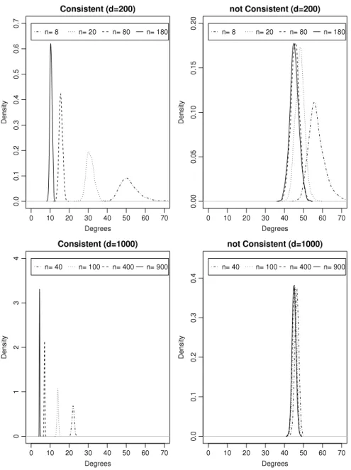
complements the results inTable 1: here we show kernel density estimates of the angles based on the 1000 iterations. The values ofnin the top row (ford

=

200) aren

=

8

,

20

,

80 and 180, and the bottom row showsn

=

40, 100, 400 and 900 for

d

=

1000. The left panels focus on the ‘‘consistent’’ columns in theTable 1, and the right panels show density estimates for the ‘‘not consistent’’ columns. These figures clearly illustrate the behavior of the angle as the sample size increases.

Returning to the ‘‘Error’’ columns inTable 1, it is noticeable that the error probability is almost 0 in the ‘‘consistent’’ cases, and is largest whennanddare both large, that is, as



bNBbecomes strongly inconsistent. For these latter results,t

=

2

/

√

n, and this choice oftmakes the discrimination problem increasingly difficult asnincreases.

8.2. Simulation II

Simulation II focuses on the performance of



δ

bof(24). As mentioned at the end of Section7, thefairapproach of Fan and

Fan [3] and thenaccapproach share the vector



bfor discrimination, but base their feature selection on different ranking

vectors:fairessentially chooses features based on(13), whilenaccselects features based on



b.

For Simulation II the parameters

µ

kandΣ0are

µ

0

=

0

∈

Rd

,

µ

1

=

(µ

11

, . . . , µ

1d

)

T

∈

Rd

,

µ

1j

=



j

/

4 j

∈ {

10

,

20

,

30

}

,

0 otherwise

.

Σ0

=

A1/2ΣA1/2

,

A

=

diag

(

ajj

),

ajj

=

j

,

andΣ is the same as in Simulation I. The mean parameters

µ

0and

µ

1show that only the 10th, 20th and 30th features

Fig. 1. Kernel density estimates of angles in degrees betweenbNBandbNB.

the covariance matrixΣ0are monotonically increasing. The observations about the large features and the behavior ofΣ0

allow us to compare the performance of thefairandnaccapproaches under a non-homogeneous variance structure of the

features.

For each pair

(

d

,

n

)

and for bothfairandnacc, we calculate estimates of the error probability as described in Simulation I. However, in this simulation, we use 100 iterations.

The estimates of the error probabilities are tabulated inTable 2, with standard deviation in parentheses. The column

d

=

200 ofTable 2shows that the error probabilities ofnaccare smaller than the corresponding values forfairexcept for n

=

10, wherefairwins. Ford

=

1000, the superiority ofnaccoverfairis apparent, especially forn

=

50

,

100

,

150

,

200. The results show the merit of feature selection with



bover that with the vector



poffair.

So far we have compared the error probabilities of the two approaches. We now look at the specific features that are selected in the simulations for

(

d

,

n

)

pairs.Fig. 2shows the frequency of the selected features over 100 simulations. The top panels show the results for

(

d

,

n

)

=

(

200

,

180

)

, and the bottom panels show similar results for

(

d

,

n

)

=

(

1000

,

180

)

. The left panels relate tonacc, and the right panels tofair. The figures show clearly thatnacccorrectly picks the large variables 10, 20 and 30 most of the time, whilefairselects many other features, typically features with a large variance. The feature

selection ofnaccis based on



band thus on

(

µ

ˆ

1j

− ˆ

µ

0j

)/

σ

ˆ

jj. Our results suggest that feature selection with



bcaptures the

Table 2

Estimated value of the error probability.

d=200 d=1000

nacc fair nacc fair

n=6 0.53167 0.53500 0.55167 0.56167 (0.26025) (0.25436) (0.23414) (0.25031) n=10 0.51100 0.50300 0.57300 0.62500 (0.20395) (0.21670) (0.24240) (0.22847) n=30 0.33933 0.35700 0.42233 0.44433 (0.13848) (0.15500) (0.17240) (0.14688) n=50 0.23360 0.25940 0.35580 0.40420 (0.08989) (0.10830) (0.13536) (0.11691) n=100 0.17510 0.19280 0.21360 0.30550 (0.04237) (0.04854) (0.08423) (0.09312) n=150 0.17993 0.18640 0.17667 0.24360 (0.03349) (0.03718) (0.04020) (0.08258) n=200 0.17035 0.17295 0.16815 0.19155 (0.02616) (0.02658) (0.02708) (0.04728) Table 3 Lung cancer data.

Method nacc fair

No. of selected genes 7 14

Selected genes 1 955 2039 2 928 34 1 136 2 039 4 345 8928 11 238 3 250 3 844 4 336 11 368 7 249 7 765 8 537 9 474 11 015 11 368 11 841 12 248 Training error 0/32 0/32 Test error 8/149 8/149

The results of Simulation II illustrate the superiority ofnaccoverfairin two ways: the error probabilities are mostly

smaller, and feature selection is more pertinent, especially for higher values ofd.

8.3. Real data

In this section, we consider the lung cancer data that were analyzed in [5]. These data are available athttp://www.

chestsurg.org/publications/2002-microarray.aspx. The data have two classes: malignant pleural mesothelioma (MPM) and

adenocarcinoma (ADCA). There are 12553 genes, the variables, and 181 samples (31 MPM and 150 ADCA). Gordon et al. [5] considered a training set of 16 MPM and 16 ADCA samples, and used the remaining 149 samples for testing. We use the same training and testing subsets.

For the lung cancer data, we comparefairwithnacc.Table 3shows the classification results of the two approaches. fairselected 14 genes, and resulted in 0 training errors and 8 test errors, whilenaccselected only 7 genes which yielded 0 training errors and 8 test errors. Both approaches select features 2039 and 11368. These features may be of interest to medical experts, but we are not concerned with this aspect in the present analysis. The results show that both classification approaches have the same number of errors, so perform equally well, butnaccfinds a more parsimonious set of features. Indeed,naccrequires only half the number of features in order to achieve the misclassification thatfairachieved.

9. Discussion

In this paper we have exhibited the relationship between canonical correlation analysis and the naive Bayes discriminant rule forhdlssdata from two classes. We showed that the estimators of the first eigenvector and the canonical correlation vector of the naive canonical correlation matrix arehdlssconsistent, providedddoes not grow too fast. Under these growth

conditions ond, the consistency results enable us to derive an upper bound for the worst case classification error which is smaller than the error previously given in [3].

Our approach, based on the naive canonical correlation matrix, naturally leads to two ranking vectors for feature selection. One of them, the eigenvector of the naive canonical correlation matrix, is equivalent to the vector Fan and Fan use in their

fair. The second candidate for feature selection, the naive canonical correlation vector, plays the dual role of also being

the natural discriminant direction for the naive Bayes rule inhdlssdata. We comparefairand our approachnacc, which uses the naive canonical correlation vector for feature selection, on simulated and real data. If the means of the two classes only differ for a small number of variables and the diagonal elements of the covariance matrix increase with the variable number (as in our Simulation II),naccperforms better thanfairboth in selecting the right features and in achieving a lower

Fig. 2. Frequency of obtained features.

classification error. In addition to the features with a nonzero mean difference,fairtypically selects features with a large

variance, whilenacc’s choice of features is not affected by the large variances.

For thehdlsslung cancer data;fairandnaccresulted in the same number of misclassified observations, however,nacc

obtained this result with only half the number of features, thus resulting in a more parsimonious model.

Forhdlssdata, the inverse of the sample covariance matrix



Σdoes not exist. To circumvent the problem caused by

the singular sample covariance matrix, we replacedΣ



by its diagonal matrix which is invertible. Instead one could use

a generalized inverse ofΣ



, and derive the ‘generalized versions’ of the vectors



pand



b. Shin and Eubank [12] consider

different Moore–Penrose generalized inverses and associated vectors



p: one based on the pooled sample covariance matrix,

and one based on the sample covariance matrix of all observations. The latter inverse and associated vector



phave some nice properties which are discussed in their paper. It would be of interest to investigate the asymptotic properties of this vector



pfor two and more classes. This will be the topic of future research.

Another possibility for overcoming the problem posed by the singular sample covariance matrix is to consider regularized canonical correlations as proposed in [9], who include smoothing parameters

α

, similar to a ridge regression parameter, in the canonical correlation setting, and then find the appropriate ‘regularized’ vectors



p_α. This solution path clearly applies tohdlsssettings, and the regularized sample solution



pαcould be used instead of our vector



pfor a suitable choice of the

Currently, our model consists of two classes. But it can be extended to general multi-class discriminant problems, which will be of interest in practice. We will pursue this in future work. Other possible research directions include extensions of our theoretical results to the ‘‘kernel method’’ in linear discrimination described in [11].

Acknowledgments

The authors would like to thank the reviewers for many helpful comments and suggestions which improved the paper. The research of the third author was supported in part by KAKENHI 23500350.

Appendix

Proof of Theorem 1. The inner product of



pand



pis

(



p

,



p

)

=

(µ

1

−

µ

0

)

TD−1/2



D−1/2

(



µ

1

−



µ

0

)



(µ

1

−

µ

0

)

TD−1

(µ

1

−

µ

0

)



(



µ

1

−



µ

0

)

T



D−1

(



µ

1

−



µ

0

)

.

(26)

From Cramér’s condition, it follows that



D

=

D

(

1

+

o_P

(

1

))

. Thus,(26)can be written as

(



p

,



p

)

=

(µ

1

−

µ

0

)

T



D−1

(



µ

₁

−



µ

₀

) (

1

+

o_P

(

1

))



(µ

1

−

µ

0

)

TD−1

(µ

1

−

µ

0

)



(



µ

1

−



µ

0

)

T_D−1

(



µ

1

−



µ

0

)

.

(27)

In particular, the denominator of(27)becomes



(



µ

1

−



µ

0

)

T_D−1

(



µ

1

−



µ

0

)

=



(µ

1

−

µ

0

)

TD−1

(µ

1

−

µ

0

)(

1

+

oP

(

1

))

+

nd n1n0

by (A.4) in [3]. On the other hand, the numerator of(27)can be decomposed as

(µ

1

−

µ

0

)

T



D −1

(



µ

1

−



µ

0

)

=

(µ

₁

−

µ

₀

)

T



D −1

(µ

1

−

µ

0

)

+

(µ

1

−

µ

0

)

T



D −1

(ε

1

−

ε

0

)

=

(µ

₁

−

µ

₀

)

T



D−1

(µ

₁

−

µ

₀

)

+

(µ

₁

−

µ

₀

)

T



D−1

ε

₁

−

(µ

₁

−

µ

₀

)

T



D−1

ε

₀

,

where

ε

1

=



n1 i=1

ε

i

/

n1and

ε

0

=



n

i=n1+1

ε

i

/

n0. From the evaluation of the termI3on p.2626 of Fan and Fan [3], we have

(µ

1

−

µ

0

)

T



D −1

(



µ

1

−



µ

0

)

=

(µ

1

−

µ

0

)

T_D−1

(µ

1

−

µ

0

) (

1

+

oP

(

1

)).

Thus,(27)becomes

(



p

,



p

)

=

1

+

oP

(

1

)



(

1

+

oP

(

1

))

+

(

n

/

n1

)

{

d

/(

n0

(µ

1

−

µ

0

)

TD−1

(µ

1

−

µ

0

))

}

=

√

1

+

oP

(

1

)

(

1

+

oP

(

1

))

+

O

(

1

)

o

(

1

)

=

1

+

oP

(

1

).

(28)

Since ‘arccos’ is a continuous function, the angle between



pand



pis

̸

(



p

,



p

)

=

arccos

(



p T



p

)

=

oP

(

1

),

and this last equality completes the proof.

Proof of Theorem 2. From(28)in the proof ofTheorem 1, and the assumptions ofTheorem 1, it follows that

(



p

,



p

)

=

1

+

oP

(

1

)

√

(

1

+

oP

(

1

))

+

ξκ(

1

+

o

(

1

))

=

√

1 1

+

ξκ

(

1

+

oP

(

1

)),

and therefore, ̸

(



p

,



p

)

=

arccos

(



p T



p

)

=

arccos



1

√

1

+

ξκ



(

1

+

oP

(

1

))

by an argument similar to that given in the proof ofTheorem 1.

Proof of Theorem 3. Using (A.4) of Fan and Fan [3],

(



µ

1

−



µ

0

)

T



D −1

(



µ

1

−



µ

0

)

=







(µ

1

−

µ

0

)

TD−1

(µ

1

−

µ

0

)(

1

+

oP

(

1

)),

d

=

o

(

nCd

),



(µ

1

−

µ

0

)

TD−1

(µ

1

−

µ

0

)

+

nd n1n0



(

1

+

oP

(

1

)),

d

=

O

(

nCd

).

On the other hand,n1

/

n

P

−→

π

andn0

/

n P

−→

1

−

π

. Therefore, the ratio of

λ

and



λ

satisfies(16). Proof of Theorem 4. The inner product

(



bNB

,



bNB

)

can be expressed as

(



bNB

,



bNB

)

=



pT_D−1/2



D−1/2



p





pTD −1



p





pT



D−1



p

=

(µ

1

−

µ

0

)

T_D−1



D−1

(



µ

₁

−



µ

₀

)



(µ

1

−

µ

0

)

TD−2

(µ

1

−

µ

0

)



(



µ

1

−



µ

0

)

T



D−2

(



µ

1

−



µ

0

)

.

Since



D

=

D

(

1

+

o_P

(

1

))

, we have

(



bNB

,



bNB

)

=

(µ

1

−

µ

0

)

T



D−2

(



µ

1

−



µ

0

)(

1

+

oP

(

1

))



(µ

1

−

µ

0

)

TD−2

(µ

1

−

µ

0

)



(



µ

1

−



µ

0

)

T_D−2

(



µ

1

−



µ

0

)

,

(29)

and we note that the numerator includes



D.

Consider the denominator of(29). We have

(



µ

1

−



µ

0

)

T_D−2

(



µ

1

−



µ

0

)

=

(µ

1

−

µ

0

)

T_D−2

(µ

1

−

µ

0

)

+

2

(µ

1

−

µ

0

)

TD−2

(ε

1

−

ε

0

)

+

(ε

1

−

ε

0

)

TD−2

(ε

1

−

ε

0

)

≡

(µ

₁

−

µ

₀

)

TD−2

(µ

1

−

µ

0

)

+

2E1

+

E2

.

(30) Now define



ε

=



n1n0 n V −1/2 R Q T RD −1/2

(ε

1

−

ε

0

),

whereVRandQRare the matrices obtained from the spectral decomposition of

R

=

QRVRQRT

.

(31)

Let

λ

R,ibe the eigenvalues ofR, soVR

=

diag

{

λ

R,1

, . . . , λ

R,d

}

. We have

{

n

/(

n1n0

)

}

GΣGT

=

Id, whereG

=

√

(

n1n0

)/

nV −1/2 R QT RD −1/2_{. Thus,}



ε

∼

Nd

(

0

,

Id

)

. On the other hand,



ε

=



n1n0 n V −1/2 R Q T RD −1/2

(ε

1

−

ε

0

)

⇐⇒

D−1

(ε

1

−

ε

0

)

=



n n1n0 D−1/2QRV 1/2 R



ε,

andE2of(30)becomes E2

=



D−1

(ε

1

−

ε

0

)



T



D−1

(ε

1

−

ε

0

)



=

n n1n0



ε

T_V1/2 R Q T RD −1_Q RV 1/2 R



ε

≤

n n1n0 max z∈Rd−{0} zT_D−1_z zT_z



QRVR1/2



ε



T



QRVR1/2



ε



=

n n1n0

λ

max

(

D−1

)



ε

T_V R



ε.

In particular,

λ

max

(

D−1

)

=

1

/

min1≤j≤d

σ

jj

<

∞

, sinceD−1is diagonal. Thus,

(ε

1

−

ε

0

)

TD−2

(ε

1

−

ε

0

)

≤

n n1n0 1 min 1≤j≤d

σ

jj



ε

T_V R



ε

=

nd n1n0 1 min 1≤j≤d

σ

jj

(

1

+

oP

(

1

))

by the weak law of large numbers.

Next, considerE1of(30), which has the distribution

(µ

1

−

µ

0

)

TD−2

(ε

1

−

ε

0

)

∼

N



0

,

n n1n0

(µ

1

−

µ

0

)

TD−2ΣD−2

(µ

1

−

µ

0

)



.

From the definition ofΓ∗_{in(18), the variance ofE}

1is evaluated as follows: V

[

E1

] =

n n1n0

(µ

1

−

µ

0

)

TD−3/2RD−3/2

(µ

1

−

µ

0

)

≤

n n1n0

λ

max

(

R

)(µ

1

−

µ

0

)

TD −3

(µ

1

−

µ

0

)

≤

n n1n0

λ

max

(

R

)λ

max

(

D−1

)(µ

1

−

µ

0

)

TD−2

(µ

1

−

µ

0

)

≤

n n1n0 b0 1 min 1≤j≤d

σ

jj

(µ

1

−

µ

0

)

TD−2

(µ

1

−

µ

0

).

Therefore, using Chebyshev’s inequality,

P









(µ

1

−

µ

0

)

TD−2

(ε

1

−

ε

0

)

(µ

1

−

µ

0

)

TD−2

(µ

1

−

µ

0

)









> ε



≤

V

[

(µ

1

−

µ

0

)

T_D−2

(ε

1

−

ε

0

)

]

{

(µ

₁

−

µ

₀

)

T_D−2

(µ

1

−

µ

0

)ε

}

2

≤



n2 n1n0







b0 min 1≤j≤d

σ

jj





1

ε

2 1 nCd

=

o

(

1

).

Consequently,

(µ

1

−

µ

0

)

TD−2

(ε

1

−

ε

0

)

=

(µ

1

−

µ

0

)

TD−2

(µ

1

−

µ

0

)

oP

(

1

)

. The previous calculations lead to the following bound for(30):

(



µ

1

−



µ

0

)

T_D−2

(



µ

1

−



µ

0

)

≤

(µ

1

−

µ

0

)

T_D−2

(µ

1

−

µ

0

)

+

2

(µ

1

−

µ

0

)

TD−2

(µ

1

−

µ

0

)

oP

(

1

)

+

1 min 1≤j≤d

σ

jj nd n1n0

(

1

+

oP

(

1

))

≤

(µ

₁

−

µ

₀

)

TD−2

(µ

1

−

µ

0

)(

1

+

oP

(

1

))

+

1 min 1≤j≤d

σ

jj nd n1n0

.

Next, we consider the numerator of(29):

(µ

1

−

µ

0

)

T



D −2

(



µ

1

−



µ

0

)

=

(µ

1

−

µ

0

)

T



D −2

(µ

1

−

µ

0

)

+

(µ

1

−

µ

0

)

T



D −2

ε

1

−

(µ

1

−

µ

0

)

T



D −2

ε

0

=

(µ

₁

−

µ

₀

)

TD−2

(µ

1

�