Title
A tensor-based Volterra series black-box nonlinear system
identification and simulation framework
Author(s)
Batselier, K; Chen, Z; Liu, H; Wong, N
Citation
Proceedings of the 35th International Conference on
Computer-Aided Design (ICCAD '16 ), Austin, TX., 7-10 November 2016, p.
Article No. 17
Issued Date
2016
URL
http://hdl.handle.net/10722/229783
A Tensor-Based Volterra Series Black-Box Nonlinear
System Identification And Simulation Framework
Kim Batselier
Department of Electrical and Electronic Engineering The University of Hong Kong
Hong Kong
Zhongming Chen
Department of Electrical and Electronic Engineering The University of Hong Kong
Hong Kong
[email protected]
Haotian Liu
Cadence Design Systems, Inc. USA
Ngai Wong
Department of Electrical and Electronic Engineering The University of Hong Kong
Hong Kong
ABSTRACT
Tensors are a multi-linear generalization of matrices to their d -way counterparts, and are receiving intense interest recently due to their natural representation of high-dimensional data and the avail-ability of fast tensor decomposition algorithms. Given the input-output data of a nonlinear system/circuit, this paper presents a non-linear model identification and simulation framework built on top of Volterra series and its seamless integration with tensor arith-metic. By exploiting partially-symmetric polyadic decompositions of sparse Toeplitz tensors, the proposed framework permits a pleas-antly scalable way to incorporate high-order Volterra kernels. Such an approach largely eludes the curse of dimensionality and allows computationally fast modeling and simulation beyond weakly non-linear systems. The black-box nature of the model also hides struc-tural information of the system/circuit and encapsulates it in terms of compact tensors. Numerical examples are given to verify the ef-ficacy, efficiency and generality of this tensor-based modeling and simulation framework.
Keywords
black box; Volterra series; nonlinear system identification; tensors; simulation
1.
INTRODUCTION
Automatic system identification and model selection of a non-linear system or circuit from a given set of input-output data is an important goal in electronic design automation (EDA). For linear systems this goal has been largely achieved, which is evident from the rich literature and many sophisticated algorithms that are avail-able, e.g., [1, 2]. In contrast, it is a much more difficult task for nonlinear systems [3].
Permission to make digital or hard copies of all or part of this work for personal or classroom use is granted without fee provided that copies are not made or distributed for profit or commercial advantage and that copies bear this notice and the full cita-tion on the first page. Copyrights for components of this work owned by others than ACM must be honored. Abstracting with credit is permitted. To copy otherwise, or re-publish, to post on servers or to redistribute to lists, requires prior specific permission and/or a fee. Request permissions from [email protected].
ICCAD ’16 Doubletree Hotel, Austin, TX, USA c
2016 ACM. ISBN XXX-XXXX-XX-XXX/XX/XX. . . $15.00 DOI:XX.XXX/XXX_X
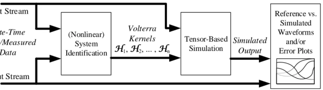
This article makes a step forward towards this goal by introduc-ing a tensor-based framework for the automatic identification and simulation of nonlinear systems and circuits with Volterra series. Our proposed framework is illustrated as a block diagram in Fig. 1. First, a set of Volterra kernelsH1,H2, . . . ,Hnare identified from
a given set of measured discrete-time input/output data. These ker-nels are then used together with a new input to generate a simulated output of the nonlinear system. We present an algorithm for both the identification and simulation block in this article. The main tool used for modeling nonlinear systems in our framework is the Volterra series, which has been successfully applied to modeling and simulating weakly nonlinear systems, e.g., [4–7]. We show that there is an inherent link between Volterra series and tensors and exploit this link to develop a fast simulation algorithm. We remark that the integration of Volterra theory and tensors has ap-peared in previous works on nonlinear simulation [8–10] and in system identification [11]. The key novelties in this work are:
• Representation of the Volterra kernels as tensors– This is not an entirely new idea and has appeared in prior work. However, we introduce, for the first time in the literature, particularToeplitz tensorsthat allow the development of a remarkably fast simulation algorithm via polyadic tensor de-compositions. The obtained reduction in required simulation runtime and storage cost is demonstrated by means of nu-merical experiments.
• Fast simulation by means of multi-mode convolution– The curse of dimensionality appears in the standard imple-mentation of Volterra kernels wherein multi-mode convolu-tions are needed in computing higher order responses. This has limited the application of Volterra series to mostly mildly nonlinear systems. Via polyadic tensor decompositions we manage to compute the multi-mode convolution by means of onlylinear convolutions, regardless of the Volterra kernel or-der. This means that strongly nonlinear systems can now be efficiently captured with high-order kernels whereby the di-mensionality curse is gratefully removed during simulation. This article is organized as follows. Section 2 reviews basic ten-sor notation and operations, followed by a succinct account on the Volterra series. The development of the nonlinear system identifi-cation and accelerated tensor-based simulation is elaborated in
Sec-tions 3 and 4. Section 5 presents three numerical examples demon-strating the efficacy of the proposed black-box modeling and sim-ulation approach. Some further remarks are given in Section 6 and Section 7 draws the conclusions.
2.
BACKGROUND
2.1
Tensors
First, we give a short introduction into the topic of tensors and the notation that we use. Tensors are denoted by boldface capital calligraphic letters (e.g. A), matrices by boldface capital letters (e.g. A), vectors by boldface letters (e.g. a), and scalars by ei-ther Roman (e.g.a) or Greek (e.g. α) letters. Thenth element in a sequence is denoted by a superscript in parentheses. For exam-ple,u(1),u(2),u(3)denote the first three elements in a sequence ofuvectors. Tensors are in our context generalizations of matri-ces and vectors. Ad-way tensorA ∈ Rn1×···×nd is simply a
d-way array. Each element of the tensorAis hence specified by
dindicesi1, . . . , idand denoted byai1···id. The positive integers
d, n1, n2, . . . , nd are called the order and the dimensions of the
tensor, respectively. Fig. 2 illustrates a3-way or 3rd-order tensor with dimensions4,3,2.
The matrix vector multiplication is generalized to the tensor case in the following way. Thek-mode product of ad-way tensorA
with a vectoru∈Rnkis defined by
(A×kuT)i1···ik−1ik+1···id=
nk X
ik=1
uikai1···ik···id.
This operation effectively removes thekth mode, resulting in a(d−
1)-way tensor. Note that for a matrixA∈Rn×nand vectoru∈ Rn, we can write the familiar matrix vector products asA×1uT ,
uTAand asA×2uT,A u.
Ad-way rank-1 tensor is the outer product ofdvectors
A=a(1)◦a(2)◦ · · · ◦a(d),
wherea(1) ∈
Rn1, . . . ,a(d) ∈ Rnd. The entries ofAare com-pletely determined byai1i2···id=a (1) i1 a (2) i2 · · ·a (d) id .
A cubical tensor is a tensor for whichn1 = n2 =· · · = nd.
A cubical tensorAis symmetric ifai1···id =aπ(i1,...,id)where
π(i1, . . . , id)is any permutation of the indices and a Toeplitz tensor
ifai1···id=ai1+1···id+1holds for all entries.
The Kronecker product [12, 13] and Hadamard product are de-noted by⊗and by respectively. We introduce the shorthand notationxd,x⊗x⊗ · · · ⊗xfor thed-times repeated Kronecker product.
An important operation on tensors is reshaping. The most com-mon reshapings are the matricization and vectorization [14], which reorder the entries ofAinto a matrixAand vector vec(A). The mode-nmatricization of a tensorArearranges the entries of A
such that the rows of the resulting matrix are indexed by thenth tensor indexin. The remaining indices are grouped in ascending
order. The only reshapings used in this paper are the mode-1 ma-tricization and vectorization.
EXAMPLE 1. The mode-1 matricization of the tensorAfrom Fig. 2 is A= 1 5 9 13 17 21 2 6 10 14 18 22 3 7 11 15 19 23 4 8 12 16 20 24 .
and its vectorization is
vec(A) = 1 2 · · · 24T .
The importance of the matricization and vectorization lies in the following two equations
A×1uT×2· · · ×nuT =vec(A)Tud (1)
and
A×2uT×3· · · ×nuT=A ud
−1
, (2)
which tell us how thek-mode products of a tensorAwith a vector
ucan be computed.
A polyadic decomposition [15, 16] of ad-way tensorAis its decomposition into a sum ofRrank-1 tensors
A =
R
X
i=1
a(1)i ◦a(2)i ◦ · · · ◦a(id).
In order to store ad-way tensorAin memory, we need to store all of itsn1× · · · ×ndelements. In contrast, storing its
polay-dic decomposition needs onlyR(n1+· · ·+nd)elements, which
can be quite a reduction whenRis small. WhenR is minimal, the polyadic decomposition is called canonical. Probably the most well-known canonical polyadic decomposition of a matrix is its sin-gular value decomposition [17]. A symmetric tensorAcan always be decomposed into a symmetric polyadic decomposition. This means that every rank-1 term is also a symmetric tensor and there-fore A = R X i=1 ai◦ai◦ · · · ◦ai.
Storage of a symmetric polyadic decomposition therefore needs onlyRnelements whenai∈Rn.
2.2
Volterra Series
Volterra theory has been developed over a century ago and has found applications in analyzing communication systems and non-linear control [4, 5]. The object of interest in this theory are the Volterra series, which can be regarded as a Taylor series with mem-ory effects since its evaluation at a particular time instance requires information from the past. Specifically, a nonlinear discrete-time time-invariant system with an inputu(t)∈Rand an outputy(t)∈ Ris described by a Volterra series as
y(t) =y1(t) +y2(t) +y3(t) +· · ·, where yn(t) = M−1 X k1=0 · · · M−1 X kn=0 hn(k1,· · ·, kn)· u(t−k1)· · ·u(t−kn), (3)
withhn(k1,· · ·, kn)thenth-order Volterra kernel andMthe
mem-ory of the kernel. We only consider causal systems, which implies thathn(k1,· · ·, kn) = 0when any of the indicesk1, . . . , kn is
negative. Note thaty1is the usual first-order convolution of the in-putu(t)with the impulse responseh1, which is well-known from linear system theory. For ordersn≥2the kernels are not unique, since the productsu(t−k1)· · ·u(t−kn)are commutative. This
becomes problematic when system properties are to be described in terms of properties of the kernels. It therefore becomes impor-tant to consider restricted forms of the kernels that impose unique-ness. The form we assume throughout this work is the symmetric
Input Stream Discrete-Time Simulated/Measured I/O Data (Nonlinear) System Identification Volterra Kernels H1, H2, ... , Hn Tensor-Based Simulation Simulated Output Reference vs. Simulated Waveforms and/or Error Plots Output Stream
Figure 1: General overview of the tensor-based black-box Volterra series identification and simulation framework.
i
1
i
2
i
3
1
5
9
2
6
10
3
7
11
4
8
12
13 17
21
14 18
22
15 19
23
16
20
24
Figure 2: An example tensorA∈R4×3×2.
one. This implies thath(k1, . . . , kn) =h(π(k1, . . . , kn)), where π(k1, . . . , kn)is any permutation of the indicesk1, . . . , kn, and
re-duces the number of distinct kernel values fromMnto MM−−1+1n ≈
(M−1)n/n!. It is straightforward to see that each Volterra kernel hncorresponds with a symmetricn-way tensorHn, which allows
us to rewrite (3) as yn(t) =Hn×1uT×2· · · ×nuT, (4) withuT= u(t) u(t−1) · · · u(t−M+ 1) . By using (1), (4) can be rewritten as yn(t) =vec(Hn)Tun= (un)Tvec(Hn), (5)
which needsO(Mn)multiplications. Defining
yn, yn(0) yn(1) · · · yn(N) T , uN, u(0) u(1) · · · u(N) T ,
we can write (5) fort= 0, . . . , Nfor a linear system(n= 1)to obtain y1= u(0) 0 · · · 0 u(1) u(0) · · · 0 .. . u(N) u(N−1) · · · u(N−M+ 1) vec(H1),
which is the well-known expression for the discrete convolution of
uN with the impulse responseH1. The convolution is here
per-formed as a matrix vector product of aN ×M Toeplitz matrix containing the values ofuN with the vectorization ofH1.
Like-wise, it is possible to rewrite the convolution as a matrix vector
2(2, 2) h h2(1,2) h2(0,2) 2(2,1) h h2(1,1) h2(0,1) 2(1,1) h 0 2(1,0) h h2(0,0) 0 0 0 0 2(0,0) h
i
1i
3i
2 2(2,0) h h2(1,0) h2(0,0) 2(0,1) h 0 0 0 0 0 0 0 0 (0) u u(1) u(2) (0) u (1) u (2) u 2(0) y 2(1) y 2(2) yFigure 3: Toeplitz tensorT2 corresponding with the Volterra
kernelh2.
product of aN×N Toeplitz matrixT1 containing the values of
H1with the vectoruNas
y1= h(0) 0 · · · 0 h(1) h(0) · · · 0 .. . . .. . .. ... .. . . .. . .. ... .. . . .. . .. ... 0 · · · h(M) · · · h(1) h(0) uN. (6)
By following the same procedure of writing (5) for an arbitraryn
for all valuest= 0, . . . , Nwe obtain
yn=Tn×2uTN×3· · · ×n+1uTN, (7)
whereTnis an+1-way cubical Toeplitz tensor of dimensionN+1
containing the coefficients of the Volterra kernelHn. Observe how
(7) reduces to (6) whenn= 1. Fig. 3 illustrates the Toeplitz tensor
Tnfor the casen = 2. We call (7) a multi-mode convolution of
uNwithHn. The computational complexity of computing such a
multi-mode convolution can be deduced from using the matriciza-tion ofTnas described in (2). Indeed, we can rewrite (7) as
yn=TnudN, (8)
=Unvec(Hn), (9)
withUnaN×Mnmatrix. Computing the multi-mode convolution
as described in (8) needsO((N+ 1)n+1)multiplications, while using (9) has a computational complexity ofO(N Mn). Since in
practiceN M, the second way is better but still suffers from the curse of dimensionality due to theMnfactor. We resolve this curse in Section 4 using a polyadic tensor decomposition. Also note that for the linear case(n= 1)the convolution can be computed using the Fast Fourier Transform (FFT) with a computational complexity ofO(NlogN).
3.
IDENTIFICATION
It is well-known that the estimation of the Volterra kernel val-ues for an unknown system from measured input/output is a linear problem. Once the values for the maximal ordernand memoryM
are chosen, one then uses the measured inputuNand outputy
sig-nal to estimate the values ofH1,H2, . . . ,Hn. By repeated use of
(9),y=y1+y2+· · ·+yncan be rewritten as the linear problem
y= U1 U2 · · · Un vec(H1) vec(H2) .. . vec(Hn) . (10) TheN×(M+M2+· · ·+Md)matrixU , U1 U2 · · · Un
introduces a constraint on how many samples need to be collected in order for the Volterra kernel values to be uniquely defined. In-deed, the matrixUis square whenN=M+M2+· · ·+Md. If more samples are measured then the linear problem can be solved using a pseudoinverse approach. Again, the curse of dimension-ality appears in the growing size of the linear system asM and
nare increased. One way to alleviate this problem somewhat is by exploiting the symmetry of each of the Volterra kernels. The vectorizationHncontains many repeated entries, which could be
removed on the condition that the corresponding values ofU are adjusted. This reduces the dimensionality of theUmatrix toN×
M+ MM−−1+21
+· · ·+ MM−−1+1n
, but does not resolves the curse. An alternative identification procedure that uses higher order ten-sors explicitly is described in [11]. Instead of identifying the sym-metric Volterra kernels, approximations to their symsym-metric polyadic decompositions are identified instead by means of three iterative al-gorithms. The estimated kernels are always approximations since the number of termsRin each of the symmetric polyadic decompo-sitions is not knowna priori. Quantifying the approximation error is difficult in this case since then one needs to compute the output to Algorithm 1 as well.
An interesting development is the use of kernel methods from machine learning in the identification of the Volterra kernels [18]. By representing the Volterra series as elements of a reproducing kernel Hilbert space, the complexity of the estimation process be-comes independent of the order of nonlinearity. Even infinite Volterra series expansions can be estimated. Whether this identification method can be used in our proposed framework requires further research. For this article, Algorithm 1 was implemented and used in the numerical experiments for prototyping and verification of the proposed ideas.
4.
SIMULATION
Once the symmetric Volterra kernels are estimated, one can use them to efficiently simulate the nonlinear system. Remember from (9) that a naive implementation of the multi-mode convolution has a computational complexity ofO(N Mn). We will illustrate how the simulation can be made significantly faster by a polyadic tensor decomposition ofHnand by exploiting the Toeplitz structure of
Tn. The main idea is that a polyadic decomposition of the Volterra
tensorHnsuffices to reconstruct the Toeplitz structure ofTn.
Sup-Algorithm 1Volterra kernel identification
Input: uN,y, M, n
Output: H1,H2, . . . ,Hn
1: forj= 1. . . ndo
2: constructUjfromuN, considering the symmetry ofHj
3: end for
4: h¯←solution of linear system (10) 5: forj= 1. . . ndo
6: extract symmetricHjtensor fromh¯vector
7: end for
Algorithm 2Fast time-domain Volterra simulation
Input: uN,H1,polyadic decompositions ofH2, . . . ,Hn
Output: y 1: y←conv(uN,H1) 2: forj= 1. . . ndo 3: fork= 1. . . jdo 4: fori= 1. . . Rdo 5: u(ik)←conv(uN, h(ik)) 6: end for 7: end for 8: y←y+PR i=1u (1) i · · · u (j) i 9: end for
pose we have a polyadic decomposition ofHn, then for a single
output sampley(t)we can rewrite equation (4) as
yn(t) =Hn×1uT×2· · · ×nuT, = ( R X i=1 h(in)◦ · · · ◦h(1)i )×1uT×2· · · ×nuT, = R X i=1 (uTh(in))· · ·(uTh(1)i ). (11)
If we now consider thekth mode and write out the inner products
uTh(ik)for allt= 0, . . . , Nwe obtain u(0) 0 · · · 0 u(1) u(0) · · · 0 .. . u(N) u(N−1) · · · u(N−M+ 1) h(ik), (12)
which is the convolution ofuN withh(ik) that can be computed
with a computational complexity ofO(NlogN). The total com-putational complexity is henceO(nRNlogN)since there aren
modes andRvectors per mode. Letu(ikk)denote the convolution
ofuN withh(ik), then (11) is computed for allt = 0, . . . , N as
yn =PRi=1u (1)
i · · · u
(n)
i . Using a symmetric polyadic
de-composition ofHncan result in an additional speedup since then
yn = PRi=1ui · · · uiwith a computational complexity of O(RNlogN). The algorithm for fast time-domain simulation us-ing polyadic decompositions of the Volterra kernels is presented in Algorithm 2. Note that the second for-loop in Algorihm 2 dis-appears when symmetric polaydic decompositions of the Volterra kernels are used.
An additional way of reducing computational complexity of Al-gorithm 2 is truncating the polyadic decomposition of eachHj.
This reduces the number of iterations of the third for-loop at the cost of introducing an approximation error.
5.
NUMERICAL EXPERIMENTS
Algorithms 1 and 2 were implemented in Matlab and tested in the following examples. We compare its runtime with the tra-ditional method of computing the multi-mode convolution. All computations were done on an Intel i5 quad-core processor run-ning at 3.3 GHz with 16 GB RAM. The polyadic and symmetric polyadic decompositions were computed with the freely available TTr1SVD [19] and STEROID [20] algorithms. The quality of the identification for unknown Volterra kernels was quantified by the mean squared error||y−yˆ||2
2/N, whereyˆdenotes the simulated output of the identified Volterra series.
5.1
Decaying multi-dimensional exponentials
First, we demonstrate the validity of Algorithms 1 and 2 by means of an artificial example. Symmetric Volterra kernels were gener-ated up to orderd= 5and with memoryM = 10and containing exponentially decaying coefficients in the following way. We first define the first-order Volterra kernels ash1(k1) = exp (−k12)withk1 = 0, .1, .2, . . . , .9. These coefficients are stored in theM×1
H1 tensor. The other remaining symmetric higher-order Volterra kernels are then generated as the following outer products ofH1
H2=H1◦H1,
H3=H1◦H1◦H1,
H4=H1◦H1◦H1◦H1,
H5=H1◦H1◦H1◦H1◦H1.
This implies that all generated symmetric Volterra kernels corre-spond, per definition, with rank-1 tensorsH2, . . . ,H5 . We also have that each entry of thenth-order Volterra kernel is given by
hn(k1, . . . , kn) = exp (−k21−k 2
2− · · · −k 2
n).
A random input signal of 4000 samples was generated from a stan-dard normal distribution. Computing the corresponding output us-ing (9) took 18 seconds. Exploitus-ing the symmetric rank-1 property of the Volterra kernels in Algorithm 2 to generate the output re-duces the computation time to 0.01 seconds, which corresponds to a speedup with a factor of 1169. The input/output signals were used in Algorithm 1 to estimate the Volterra kernels. Since the correct Volterra kernels are known in this case, we use the relative identifi-cation error to quantify the accuracy of our identifiidentifi-cation algorithm. The relative identification error is defined as
||Hk−Hˆk||F
||Hk||F ,
whereHˆk denotes the estimated Volterra kernel and||X||F
de-notes the Frobenius norm of a tensorX (the square root of the sum of squares of all entries inX). Table 1 lists the relative iden-tification errors for each order of the estimated Volterra kernels, confirming the validity of Algorithm 1.
Table 1: Relative identification errors - decaying exponentials.
order 1 2 3 4 5
error 8.6e−8 1.0e−8 5.9e−10 1.0e−11 4.2e−13
5.2
Nonlinear inductance
Next, we consider a nonlinear inductance which is described by
v= 0.02 (1−(tanh2(i/5))di dt,
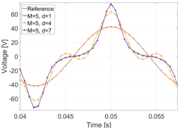
Figure 4: Output voltage of the nonlinear inductance for Volterra series of maximal order1,4,7.
wherevis the output voltage andiis the input current. A 60Hz sinusoidal current and its corresponding voltage were sampled at 100kHz for 0.1 seconds. Volterra kernels were estimated by Algo-rithm 1 with memoriesMranging from 1 to 5 and ordersdfrom 1 up to 7. Fig. 4 shows one period of the simulated output voltage for different orders of the Volterra kernel. Table 2 lists the mean squared error of the output voltage for all identified Volterra series. Notice how the mean squared error is independent fromM when
d <7and decreases as soon as an extra odd order is included in the Volterra series. Ford= 7a steady decrease of the mean squared error is observed as a function ofM. A7th-order Volterra series with memoryM = 5manages to model the output voltage with a mean squared error of0.0063.
Table 2: Mean squared error - nonlinear inductance.
H H H HH d M 1 2 3 4 5 1 .339 .162 .162 .162 .162 2 .339 .162 .162 .162 .162 3 .339 .061 .061 .061 .061 4 .339 .061 .061 .061 .061 5 .339 .021 .021 .020 .020 6 .339 .021 .021 .020 .020 7 .339 .009 .008 .007 .006
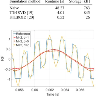
Several input series were then used to compare the different sim-ulation methods. Table 3 lists the typical runtime and storage cost for one set using three different simulation methods on the7 th-order Volterra series with memoryM = 5. The ‘naive’ method computes the multi-mode convolution using (9). TTr1SVD and STEROID use Algorithm 2 with the respective polyadic and sym-metric polyadic decompositions of the Volterra tensors. The larger storage requirement for the TTr1SVD method is due to that each
ith Volterra kernel requires the storage ofimode vectors, while STEROID only needs to store only one vector for every term. The STEROID method is superior compared to the two other simulation methods with a speedup of 93 in runtime compared to the naive method and a reduction of required storage by a factor of 29.
5.3
Double balanced mixer
In this example we consider a double balanced mixer used for upconversion. The output RF signal is determined by the input LO
Table 3: Runtimes and storage costs - nonlinear inductance.
Simulation method Runtime [s] Storage [kB]
Naive 48.27 763
TTr1SVD [19] 4.01 845
STEROID [20] 0.52 26
Figure 5: Output RF signal of the mixer for Volterra series of maximal order1,5,7.
and IF signals. All signals were sampled at 10 kHz for 1 second. The LO and IF signals have frequencies of 600 and 100 Hz respec-tively, with a phase difference ofπ/8. Again, Volterra kernels were estimated by Algorithm 1 with memories ranging from 1 to 5 and orders from 1 up to 7. Table 4 lists the mean squared error of the RF output signal as a function ofMandd. One needs a minimal order and memory of 6 and 2 respectively in order to see a decrease in the mean squared error. The mean squared error seems to be small even for the linear system, however, these models are not able to capture the high frequency variations that are relatively small in amplitude while the Volterra series can.
Table 4: Mean squared error - double balanced mixer.
H H H HH d M 1 2 3 4 5 1 .006 .006 .006 .006 .006 2 .006 .006 .006 .006 .006 3 .006 .006 .006 .006 .006 4 .006 .006 .006 .006 .006 5 .006 .006 .006 .006 .006 6 .006 .003 .003 .003 .003 7 .006 .003 .003 .003 .003
Fig. 5 shows one period of the simulated output RF signal for different orders of the Volterra kernel. Notice the small difference between the simulated output of the linear and5th-degree Volterra series, indicating the high nonlinearity of the mixer. A6th-degree Volterra series with memoryM = 2is able to follow the high frequency RF output. Increasing the memoryMor orderddid not lead to any further improvement of the simulated output. Again, the same input/output series were used for comparing the different simulation methods for thed= 6,M = 2model. Table 5 lists the runtime and storage cost for the three different simulation methods. The same patterns as in the previous example can be observed. The TTr1SVD method needs more storage due to the increasing number
of mode vectors that it needs to store. The STEROID method is far superior with a speedup of 266 in runtime compared to the naive method and needing only about one third of the storage.
Table 5: Runtimes and storage costs - double balanced mixer.
Simulation method Runtime [s] Storage [kB]
Naive 5.749 0.98
TTr1SVD [19] 0.081 2.11
STEROID [20] 0.021 0.39
6.
REMARKS
Some key contributions are summarized again:
1. The (symmetric) polyadic tensor decomposition effectively breaks down the multi-mode convolution of an input vector with any higher order Volterra kernel into purely linear con-volutions. Tensor decompositions are therefore key in over-coming the curse of dimensionality.
2. Continuing from the previous remark, the relatively expen-sive tensor decomposition computation is done onlyonce and is the overhead to pay. The simulation algorithm then benefits from the recurring and cheap linear convolution op-eration.
3. The least-squares framework for kernel identification as de-scribed by (10), though being effective, is generic to this work and is employed due to its ease of implementation for validating ideas. Other, more sophisticated, Volterra ker-nel identification methods can be readily substituted for ro-bust Volterra kernel identification subject to, say, noisy input-output samples.
4. The identified Volterra kernels completely hide the circuit or topological details, while allowing efficient user black-box simulation via compact tensor mode factor representation. In other words, the proposed framework also suggests an effec-tive means of intellectual property (IP) protection.
5. The proposed framework now handles only the identifica-tion and simulaidentifica-tion of single-input single-output (SISO) sys-tems. The extension to the direct handling of multiple-input multiple-output (MIMO) data streams is underway. More-over, research is being conducted on the characterization of stability and passivity of the identified models.
7.
CONCLUSIONS
This paper has proposed a highly efficient black-box identifica-tion and simulaidentifica-tion framework for nonlinear systems/circuits based solely on the provision of discrete-time input-output samples. A natural link has been established between Volterra kernels, multi-mode convolution and tensor decompositions. A new tensor-based Volterra simulation algorithm has been developed. Numerical ex-amples have been given to demonstrate the significant reduction in runtime and required storage cost for the simulation of some highly nonlinear systems. Compared to conventional Volterra-based sim-ulation, a runtime speedup up to 1000×and a decrease in storage up to 29×have been observed.
8.
REFERENCES
[1] L. Ljung, Ed.,System Identification (2Nd Ed.): Theory for the User. Upper Saddle River, NJ, USA: Prentice Hall PTR, 1999.
[2] T. Katayama,Subspace Methods for System Identification, ser. Communications and Control Engineering. Springer London, 2005.
[3] O. Nelles,Nonlinear System Identification: From Classical Approaches to Neural Networks and Fuzzy Models, ser. Engineering online library. Springer, 2001.
[4] W. Rugh,Nonlinear System Theory – The Volterra-Wiener Approach. Baltimore, MD: Johns Hopkins Univ. Press, 1981.
[5] E. Bedrosian and S. O. Rice, “The output properties of Volterra systems (nonlinear systems with memory) driven by harmonic and Gaussian inputs,”Proc. IEEE, vol. 59, no. 12, pp. 1688–1707, Dec. 1971.
[6] J. R. Phillips, “Projection-based approaches for model reduction of weakly nonlinear time-varying systems,”IEEE Trans. Comput.-Aided Design Integr. Circuits Syst., vol. 22, no. 2, pp. 171–187, Feb. 2003.
[7] P. Li and L. Pileggi, “Compact reduced-order modeling of weakly nonlinear analog and RF circuits,”IEEE Trans. Comput.-Aided Design Integr. Circuits Syst., vol. 24, no. 2, pp. 184–203, Feb. 2005.
[8] R. Boyer, R. Badeau, and G. Favier, “Fast orthogonal decomposition of Volterra cubic kernels using oblique unfolding,” inProc. Very Large Scale Integration (VLSI-SoC), Oct. 2011, pp. 160–163.
[9] G. Favier and T. Bouilloc, “Parametric complexity reduction of Volterra models using tensor decompositions,” in17th European Signal Processing Conference (EUSIPCO), Aug 2009.
[10] H. Liu, X. Y. Z. Xiong, K. Batselier, L. Jiang, L. Daniel, and N. Wong, “STAVES: Speedy tensor-aided volterra-based
electronic simulator,” inComputer-Aided Design (ICCAD), 2015 IEEE/ACM International Conference on, Nov 2015, pp. 583–588.
[11] G. Favier, A. Y. Kibangou, and T. Bouilloc, “Nonlinear system modeling and identification using
Volterra-PARAFAC models,”Int. J. Adapt. Control Signal Process, vol. 26, no. 1, pp. 30–53, Jan. 2012.
[12] P. A. Regalia and M. K. Sanjit, “Kronecker products, unitary matrices and signal processing applications,”SIAM Review, vol. 31, no. 4, pp. 586–613, 1989.
[13] C. F. V. Loan, “The ubiquitous Kronecker product,”J. Comp. Appl. Math., vol. 123, no. 1-2, pp. 85–100, Nov. 2000. [14] T. Kolda and B. Bader, “Tensor decompositions and
applications,”SIAM Review, vol. 51, no. 3, pp. 455–500, 2009.
[15] J. D. Carroll and J. J. Chang, “Analysis of individual differences in multidimensional scaling via an n-way generalization of “Eckart-Young” decomposition,” Psychometrika, vol. 35, no. 3, pp. 283–319, 1970.
[16] R. A. Harshman, “Foundations of the PARAFAC procedure: Models and conditions for an “explanatory” multi-modal factor analysis,”UCLA Working Papers in Phonetics, vol. 16, no. 1, p. 84, 1970.
[17] G. H. Golub and C. F. V. Loan,Matrix Computations, 3rd ed. The Johns Hopkins University Press, Oct. 1996.
[18] M. O. Franz and B. Schölkopf, “A unifying view of Wiener and Volterra theory and polynomial kernel regression,” Neural Computation, vol. 18, no. 12, pp. 3097–3118, 2006. [19] K. Batselier, H. Liu, and N. Wong, “A constructive algorithm
for decomposing a tensor into a finite sum of orthonormal rank-1 terms,”SIAM Journal on Matrix Analysis and Applications, vol. 26, no. 3, pp. 1315–1337, Sep. 2015. [20] K. Batselier and N. Wong, “Symmetric tensor decomposition
by an iterative eigendecomposition algorithm,”ArXiv e-prints, Sep. 2014.