Factoring polynomials via polytopes
∗ Fatima Abu Salem†, Shuhong Gao‡and Alan G.B. Lauder§January 7, 2004
Abstract
We introduce a new approach to multivariate polynomial factori-sation which incorporates ideas from polyhedral geometry, and gener-alises Hensel lifting. Our main contribution is to present an algorithm for factoring bivariate polynomials which is able to exploit to some extent the sparsity of polynomials. We give details of an implemen-tation which we used to factor randomly chosen sparse and composite polynomials of high degree over the binary field.
1
Introduction
Factoring polynomials is a fundamental problem in algebra and number theory and it is a basic routine in all major computer algebra systems. There is an extensive literature on this problem; for an incomplete list of references see [2, 3, 4, 12, 15, 17, 22, 24, 27] for univariate polynomials and [5, 7, 11, 14, 16, 18, 19, 20, 21, 23, 25, 26] for multivariate polynomials. Most of these papers deal with dense polynomials, except for two of them [11, 18]. The latter two papers reduce sparse polynomials with more than two variables to bivariate or univariate polynomials which are then treated as dense polynomials. It is still open whether there is an efficient algorithm
∗Fatima Abu Salem is supported by the EPSRC, Shuhong Gao is partially supported
by the NSF, NSA and ONR, and Alan Lauder is a Royal Society University Research Fellow. Mathematics Subject Classification 2000: Primary 14Q10, 11Y99. Key words and phrases: multivariate polynomial, factorisation, algorithm, Newton polytope.
†Oxford University Computing Laboratory, Wolfson Building, Parks Road, Oxford
OX1 3QD, U.K. E-mail: [email protected]
‡Department of Mathematical Sciences, Clemson University, Clemson, SC 29634-0975,
USA. E-mail: [email protected].
§Mathematical Institute, Oxford University, Oxford OX1 3LB, U.K. E-mail:
for factoring sparse bivariate or univariate polynomials. Our goal in this paper is to study sparse bivariate polynomials using their connection to integral polytopes.
Newton polytopes of multivariate polynomials reflect to a certain extent the sparsity of polynomials and they carry a lot of information about the factorization patterns of polynomials as demonstrated in our recent work [6, 8]. In [9], we deal with irreducibility of random sparse polynomials. In this paper our focus is on the more difficult problem of factoring sparse poly-nomials. We do not solve this problem completely. However, our approach is a practical new method which generalises Hensel lifting; its running time will in general improve upon that of Hensel lifting and sparse bivariate poly-nomials can often be processed significantly more quickly. As with Hensel lifting it has an exponential worst-case running time.
Here is a brief outline of the paper. In Section 2 we present a brief intro-duction to Newton polytopes and their relation to multivariate polynomials, and in Section 3 we state our central problem. Section 4 contains an outline of our method, and highlights the theoretical problems we need to address. The main theorem underpinning our method is proved in Section 6, after a key geometric lemma in Section 5. Section 7 contains a concise description of the algorithm. Finally in Section 8 we present a small example, as well as details of our computer implementation of the algorithm. We believe the main achievements of this paper are the theoretical results in Section 6, and the high degree polynomials we have factored using the method, as presented in Subsection 8.2.
2
Newton polytopes and Ostrowski’s theorem
This paper considers polynomial factorisation over a field F of arbitrary characteristic. We denote byN thenon-negative integers, andZ,Q and R the integers, rationals and reals.
Let F[X1, X2, . . . , Xn] be the ring of polynomials in n variables over
the field F. For any vector e= (e1, . . . , en) of non-negative integers define Xe :=Xe1
1 . . . Xnen. Letf ∈F[X1, . . . , Xn] be given by
f :=!
e
aeXe
where the sum is over finitely many pointseinNn, andae∈F. The Newton polytope of f, Newt(f), plays an essential role in all that follows. It is the
corresponding coefficientae is non-zero. It has integer vertices, since all the
eare integral points; we call such polytopes integral. Given two polytopes Qand R theirMinkowski sumis defined to be the set
Q+R:={q+r|q∈Q, r∈R}.
When Q and R are integral polytopes, so is Q+R. If we can write an
integral polytope P as a Minkowski sum Q+R for integral polytopes Q
and R then we call this an(integral) decomposition. The decomposition is
trivial if Q or R has only one point. The motivating theorem behind our
investigation is (see [6]):
Theorem 1 (Ostrowski) Let f, g, h ∈ F[X1, . . . , Xn]. If f = gh then
Newt(f) = Newt(g) + Newt(h).
An immediate result of this theorem relates to testing polynomial irre-ducibility: In the simplest case in which the polytope does not decompose, one immediately deduces that the polynomial must be irreducible. This was explored in [6, 8, 9], in particular a quasi-polynomial time algorithm is presented in [9] for finding all the decompositions of any given integral polytope in a plane. In this paper, we address the more difficult problem: Given a decomposition of the polytope, how can we recover a factorisation of the polynomial whose factors have Newton polytopes of that shape, or show that one does not exist?
In the remainder of the paper, we restrict our attention to bivariate polynomials, andf always denotes a bivariate polynomial in the ringF[x, y].
For e = (e1, e2) ∈ N2, we redefine the notation Xe to mean xe1ye2. We
shall retain the term “Newton polytope” for the polygon Newt(f) to avoid
confusion with other uses of the term “Newton polygon”.
3
Extending Partial Factorisations
Let Newt(f) =Q+R be a decomposition of the Newton polytope off into
integral polygons in the first quadrant. For each lattice point q ∈ Q and r∈R we introduce indeterminatesgq and hr. The polynomialsgand h are then defined as
g := "q∈QgqXq
h := "r∈RhrXr.
We callgandhthegenericpolynomials given by the decomposition Newt(f)
The equation f = gh defines a system of #Newt(f) quadratic equations
in the coefficient indeterminates obtained by equating coefficients of each monomial Xe with e∈ Newt(f) on both sides. The aim is to find an effi -cient method of solving these equations for field elements. Our approach, motivated by Hensel lifting, is to assume that, along with the decomposi-tion of the Newton polytope, we are given appropriate factorisadecomposi-tions of the polynomials defined along its edges. This “boundary factorisation” of the polynomial is then “lifted” into the Newton polytope, and the coefficients of the possible factorsgand h revealed in successive layers. Unfortunately, to
describe the algorithm properly we shall need a considerable number of ele-mentary definitions — the reader may find the figures in Section 8.1 useful in absorbing them all.
Let S be a subset of Newt(f). An S-partial factorisationof f is a
spe-cialisation of a subset of the indeterminates gq and hr such that for each lattice points∈S the coefficients of monomials Xs in the polynomials gh and f are equal field elements. (A specialisation is just a substitution of
field elements in place of indeterminates.) The caseS = Newt(f) is
equiv-alent to a factorisation off in the traditional sense, and we will call this a
full factorisation. Now suppose we have an S-partial factorisation and an
S′-partial factorisation. Suppose furtherS⊆S′and the indeterminates
spe-cialised in theS-partial factorisation have been specialised to the same field
elements as the corresponding ones in theS′-partial factorisation. Then we
say theS′-partial factorisation extends the S-partial factorisation. We call
this extensionproperifS′ has strictly more lattice points thanS.
Let Edge(f) denote the set of all edges of Newt(f). Any rational affine
functionall on R2 may be written as
l: (r1, r2)$→ν1r1+ν2r2+η.
whereν1,ν2,η∈Q. Givenδ∈Edge(f), letlδbe the unique affine functional
such that
δ={r= (r1, r2)∈Newt(f)|lδ(r) = 0}
and ν1,ν2,η ∈ Z, gcd(ν1,ν2) = 1 with Newt(f) lying in the non-negative
halfplane
{r ∈R2|lδ(r)≥0}.
(The first two conditions specify this functional up to the sign of its first co-efficient, and the final condition specifies the sign). We calllδthenormalised
Let Γ ⊆Edge(f), and let K = (kγ)γ∈Γ be a vector of positive integers labelled byΓ. Define
Newt(f)|Γ,K :={e∈Newt(f)|0≤lγ(e)< kγ for someγ ∈Γ}.
This defines a strip along the interior of Newt(f), or a union of such strips.
For eachδ∈Edge(f), there exists a unique pair of faces (either edges or
vertices)δ′ and δ′′ of Qand R respectively such thatδ =δ′+δ′′. One can
also easily show that there exists a unique integercδ such that
δ′ = {q∈Q|lδ(q) =cδ}
δ′′ = {r∈R|lδ(r) =−cδ+η}
where η = lδ(0). We denote by Q|Γ,K and R|Γ,K the subsets of Q and R respectively given by
Q|Γ,K := {e∈Q|0≤lδ(e)< kδ+cδ for someδ∈Γ} R|Γ,K := {e∈R|0≤lδ(e)< kδ−cδ+η for someδ ∈Γ}.
Once again these denote strips along the inside of Q and R whose sum
contains the strip Newt(f)|Γ,K in Newt(f).
We now come to the main definition of this section.
Definition 2 ANewt(f)|Γ,K-factorisation is called a(Γ, K;Q, R)-factorisation
if the following two properties hold:
• Exactly the indeterminate coefficients of g and h indexed by lattice
points in Q|Γ,K andR|Γ,K, respectively, have been specialised.
• Let K′ = (kγ′)γ∈Γ be a vector of positive integers with k′γ ≥kγ for all
γ∈Γ, with the inequality strict for at least one γ. Then not all of the
indeterminate coefficients of gindexed by lattice points in Q|Γ,K′ have
been specialised.
The second property will be used only once, in the proof of Lemma 8. In most instancesQ, RandΓwill be clear from the context. If so we will
omit them and refer simply to a K-factorisation. Furthermore, if K is the
all ones vector, denoted (1), of the appropriate length indexed by elements of some setΓ, then we call this a (Γ;Q, R)-boundary factorisation. We shall
simplify this to partial boundary factorisation or (1)-factorisation when Γ,
QandR are evident from the context. This special case will be the “lifting
The central problem we address is
Problem 3 Let f ∈ F[x, y] have Newton polytope Newt(f) and fix a
Minkowski decomposition Newt(f) = Q+R where Q and R are integral
polygons in the first quadrant. Suppose we have been given a (Γ;Q, R
)-boundary factorisation of f for some set Γ ⊆ Edge(f). Construct a full
factorisation off which extends it, or show that one does not exist.
Moreover, one wishes to solve the problem in time bounded by a small polynomial function of #Newt(f).
4
The Polytope Method
4.1 An outline of the method
We now give a basic sketch of our polytope factorisation method for bivariate polynomials. Throughout this section Γ will be a fixed subset of Edge(f)
and Newt(f) =Q+Ra fixed decomposition. We shall need to place certain
conditions onΓ later on, but for the time being we will ignore them. Since
Γ, Qand Rare fixed we shall use our abbreviated notation when discussing
partial factorisations.
We begin withK = (1) the all-ones vector of the appropriate length and
a K-factorisation (partial boundary factorisation). Recall this is a partial
factorisation in which exactly the coefficients in the sets Q|Γ,K and R|Γ,K, subsets of points on the boundaries ofQand R, have been specialised.
At each step of the algorithm we either show that no full factorisation of
f exists which extends this partial factorisation, and halt. Or that at most
one can exist, and we find a newK′-factorisation withK′ = (kδ′) such that
!
δ∈Γ
k′δ>! δ∈Γ
kδ.
(Usually the sum will be incremented by just one.) Iterating this procedure either we halt after some step, in which case we know that no factorisation of f exists which extends the original partial boundary factorisation. Or
we eventually have Newt(f) ⊆ Newt(f)|Γ,K, for the updated K (or just
Q⊆Q|Γ,K orR ⊆R|Γ,K will do). At that point all of the indeterminates in our partial factors have been specialised, and we may check to see if we have found a pair of factors by multiplication. (In the case, say, that just
Q⊆Q|Γ,K we only know that the partial factorg has all of its coefficients specialised, so we may use division to see if this is a factor.)
Note that in the situation in which Newt(f) is just a triangle with
ver-tices (0, n),(n,0) and (0,0) for somen, our method reduces to the standard
Hensel lifting method for bivariate polynomial factorisation. As such, our “polytope method” is a natural generalisation of Hensel lifting from the case of “generic” dense polynomials to arbitrary, possibly sparse, polynomials.
4.2 Hensel lifting equations
In this section we derive the basic equations which are used in our algorithm. For any δ ∈ Edge(f) recall that lδ is the associated normalised affine
functional. Fori≥0 we define
fiδ:= !
lδ(e)=i
aeXe.
Thusfiδis just the polynomial obtained fromf by removing all terms whose
exponents do not lie on the “ith translate of the supporting line of δ into
the polytope Newt(f)”. We call the polynomials fδ
0 edge polynomials.
Given the decomposition Newt(f) = Q+R let δ′ and δ′′ denote the unique faces ofQandRwhich sum to giveδ. As before assume “lδ(δ′) =cδ”
and “lδ(δ′′) =−cδ+η”. Letgandhdenote generic polynomials with respect
toQand R. For i≥0 define
giδ := ! q∈Q, lδ(q)=cδ+i gqXq hδi := ! r∈R, lδ(r)=−cδ+η+i hrXr. Once againgδ
i and hδi are obtained from g and h by considering only those terms which lie on particular lines. The next result is elementary but fun-damental.
Lemma 4 Let f ∈ F[x, y] and Newt(f) = Q+R be an integral
decompo-sition with corresponding generic polynomialsg and h. Let Edge(f) denote
the set of edges of Newt(f) and δ ∈ Edge(f). The system of equations in
the coefficient indeterminates of g and h defined by equating monomials on
both sides of the equality f = gh has the same solutions as the system of
equations defined by the following:
f0δ=g0δhδ0, and gδ0hδk+hδ0gδk=fkδ−
k−1
!
j=1
Thus any specialisation of coefficient indeterminates which is a solution of
equations (1) will give a full factorisation off.
Proof: In the equationf =ghgather together on each side all
monomi-als whose exponent vectors lie on the same translate of the line supporting
δ.
These are precisely the equations which are used in Hensel lifting to try and reduce the non-linear problem of selecting a specialisation of the coefficients of g and h to give a factorisation of f, to a sequence of linear
systems which may be recursively solved. We recall precisely how this is done, as our method is a generalisation.
We begin with a specialisation of the coefficients in the polynomials gδ 0
and hδ0 which yields a full factorisation of the polynomial f0δ. Equation (1)
with k = 1 gives a linear system for the indeterminate coefficients of g1δ
and hδ
1. In the special case in which standard Hensel lifting applies this
system may be solved uniquely, and thus a unique partial factorisation off
is defined which extends the original one. This process is iterated fork >1
until all the indeterminate coefficients in one of the generic polynomials have been specialised, at which stage one checks whether a factor has been found by division.
The problem with this method is that in general there may not be a unique solution to each of the linear systems encountered. There will be a unique solution in the dense bivariate case mentioned at the end of Section 4.1, subject to a certain coprimality condition. General bivariate polyno-mials may be reduced to ones of this form by randomisation, but the sub-stitutions involved destroy the sparsity of the polynomial. Our approach avoids this problem, although again is not universal in its applicability. As explained earlier, our method extends a special kind of partial boundary factorisation of f, rather than just the factorisation of one of its edges. In
this way uniqueness in the bivariate case is restored.
5
A Geometric Lemma
This section contains a geometric lemma which ensures our method can proceed in a unique way at each step provided we start with a special type of partial boundary factorisation. We begin with a key definition.
Definition 5 Let Λbe a set of edges of a polygonP in R2 andra vector in
hold:
• P is contained in the Minkowski sum of the set∪λ∈Λλand the infinite
line segment rR≥0 (the positive hull of r). Call this sum Mink(Λ, r).
• Each of the two infinite edges of Mink(Λ, r) contains exactly one point
of P.
Thus Mink(Λ, r) comprises a region bounded by the interior strip
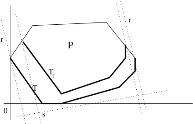
be-tween its two infinite edges and all edges inΛ. This definition is illustrated in Figure 1 whereΛconsists of all the bold edges on the boundary indicated byT. T1 s r r T 0 P
Figure 1: Dominating set of edges
We will call Λ an irredundant dominating set if it is a dominating set which does not strictly contain any other dominating set. The edges in an irredundant dominating set are necessarily connected. For a polygonP in R2, it is obvious that there exists at least one such irredundant
dominat-ing set, namely, the set comprisdominat-ing all edges connectdominat-ing the leftmost and rightmost, or the highest and lowest vertices ofP.
The next lemma is at the heart of our algorithm.
Lemma 6 Let P be an integral polygon and Λ an irredundant dominating
set of edges ofP. SupposeΛ1 is a polygonal line segment inP such that each
edge ofΛ1 is parallel to some edge ofΛ. IfΛ1 is different fromΛthenΛhas
at least one edge that has strictly more lattice points than the corresponding
The lemma is illustrated in Figure 1, where T denotes the union of the
edges inΛ and T1 the union of the line segments inΛ1.
Before proving this lemma we make one more definition. We define a mapπronto the orthogonal complement⟨r⟩⊥:={s∈R2|(s·r) = 0}of the vectorr as follows: πr(v) =v− #v·r r·r $ r.
We call thisprojection by r, and we have that πr(P) = πr(Λ). Notice that ife1 and e2 are adjacent edges in an irredundant dominating set, then the
length of the projection by r of the polygonal line segmente1e2 is just the
sum of the lengths of the projections byr of the individual edgese1 ande2.
For otherwise, we would have, say,πr(e1)⊆πr(e2) and hence the Minkowski
sum of the positive hull ofr ande1 would lie within that ofr and e2. Thus
the edge e1 would be redundant, a contradiction. The same is true if we
replacee1 and e2 by any adjacent line segments parallel to them — we still
obtain an “additivity” in the lengths, which shall be used in the proof of the lemma.
Proof: We assume that Λ dominates P in the direction r as shown in
Figure 1. Letδ1,· · ·,δk be the edges inΛ and δ1′,· · ·,δ′k the corresponding edges ofΛ1. Let ni be the number of lattice points on δi, and mi that on
δ′i, 1≤i≤k. We want to show that ni > mi for at least one i, 1≤i≤k. Suppose otherwise, namely
ni ≤mi, 1≤i≤k. (2)
We derive a contradiction by considering the lengths of Λ and Λ1 on the
projection byπr. Note that if mi = 0 for someithen certainlyni> mi and we are done; thus we may assume thatmi≥1 for all i.
First, certainly π(Λ1) ⊆ π(Λ) as Λ is a dominating set. Since Λ1 is
different from Λ, their corresponding end points must not coincide. Hence at least one end point ofΛ1 will not be on the infinite edges in the direction r. Hence πr(Λ1) lies completely inside πr(Λ), so has length strictly shorter thanπr(Λ).
Now for 1≤i≤kletϵi be the length of the projection of a primitive line segment on δi (which means that the line segment has both end points on lattice points but no lattice points in between). Certainlyϵi ≥0. Since the end points of δi are lattice points, the length of πr(δi) is exactly (ni−1)ϵi for 1≤i≤k, henceπr(Λ) has length"ki=1(ni−1)ϵi. (Here we need the fact that the dominating set is irredundant, to give us the necessary “additivity” in the lengths.) For δi′, since it is parallel to δi, the projected length of a
primitive line segment on it is alsoϵi. Hence the length ofπr(Λ1) is at least
"k
i=1(mi−1)ϵi and from (2) we know that k ! i=1 (mi−1)ϵi≥ k ! i=1 (ni−1)ϵi.
This contradicts our previous observation thatπr(Λ1) is strictly shorter than
πr(Λ). The lemma is proved.
6
The Main Theorem
Let Γ be an irredundant dominating set of Newt(f). We call a (Γ;Q, R
)-boundary factorisation off adominating edges factorisationrelative toΓ, Q
and R. A coprime dominating edges factorisation is a (Γ;Q, R)-boundary
factorisation with the property that for each δ ∈ Γ the edge polynomials g0δ and hδ0 are coprime, up to monomial factors. (In other words, they are
coprime as Laurent polynomials. Note that our factorisation method applies most naturally to Laurent polynomials.)
We are now ready to state our main theoretical result.
Theorem 7 Let f ∈ F[x, y] and Newt(f) = Q+R be a fixed Minkowski
decomposition, whereQandRare integral polygons in the first quadrant. Let
Γ be an irredundant dominating set of Newt(f) in direction r, and assume
that Q is not a single point or a line segment parallel to rR≥0. For any
coprime dominating edges factorisation of f relative to Γ, Q and R, there
exists at most one full factorisation off which extends it, and moreover this
full factorisation may be found or shown not to exist in time polynomial in
#Newt(f).
We shall prove this theorem inductively through the next two lemmas.
Lemma 8 Let f, Q, RandΓ be as in the statement of Theorem 7. Suppose
we are given a K-factorisation of f, where K = (kδ)δ∈Γ (more specifically,
a (Γ, K;Q, R)-factorisation). For each δ ∈ Γ, denote by δ′ the face of Q
supported by lδ−cδ. There exists δ∈Γ with the following properties
• The faceδ′ is an edge (rather than a vertex).
• The number of unspecialised coefficients of gδkδ is non-zero but strictly
• All the unspecialised terms have exponents which are adjacent integral
points on the line defined by the vanishing of lδ−cδ+kδ.
Proof: Let ¯Qbe the polygon
¯
Q:={r ∈Q|lδ(r)≥cδ+kδ for all δ∈Γ}.
Note that the lattice points in ¯Qcorrespond to unspecialised coefficients of g. Let Λ denote the set of edgesδ ∈Γ of Newt(f) such that the functional lδ−cδ supports an edge ofQ (rather than just a vertex). Note thatΛ̸=∅,
for otherwise Q must be a single point or a line segment in direction r,
contradicting our assumption. We denote the edge by δ′, and write ¯δ for
the face of ¯Q supported bylδ−cδ+kδ. Note that each ¯δ contains at least
one lattice point. (This follows from the second property in Definition 2.) Certainly, ¯δ is parallel to δ′ for eachδ ∈Λ, and the edge sequence {δ¯}δ∈Λ, forms a polygonal line segment inQ. Since Γis an irredundant dominating
set for Newt(f), the set of edges {δ′}δ∈Λ is an irredundant dominating set forQ. By Lemma 6, there is at least one edgeδ ∈Λ, such thatδ′ has strictly
more lattice points than ¯δ. This edge δ has the required properties. This
completes the proof.
Lemma 9 Let f, Q, RandΓ be as in the statement of Theorem 7. Suppose
we are given aK-factorisation off, where K= (kδ)δ∈Γ. Moreover, assume
this factorisation extends a coprime dominating edges factorisation, i.e., the
polynomials gδ0 and hδ0 are coprime up to monomial factors for all δ ∈ Γ.
Then there existsδ ∈Γsuch that the coefficients ofgkδδ are not all specialised,
but they may be specialised in at most one way consistent with equations (1).
This specialisation may be computed in time polynomial in#Newt(f).
Proof: Select δ ∈Γ such that the properties in Lemma 8 hold. Let nδ
andmδ be the number of integral points on the edgesδ′ and ¯δ respectively,
whereδ′and ¯δare defined as in the proof of Lemma 8. Thus we havemδ < nδ
andmδ≥1. Writelδ(e1, e2) =ν1e1+ν2e2+η, whereν1 andν2 are coprime.
Thus there exist coprime integers ζ1 and ζ2 such that ζ1ν1+ζ2ν2 = 1, and
they are unique under the requirement that 0 ≤ ζ2 < ν1. First, we shall
perform a “unimodular change of basis” on our exponents to transform our lifting equations (1) into a more convenient form.
Define the change of variables z:=xν2y−ν1 and w:=xζ1yζ2. Note that
any monomial of the formxe1ye2 can be written as xe1ye2 =zi1wi2
where
i1 =e1ζ2−e2ζ1, i2=e1ν1+e2ν2 =lδ(e1, e2)−η.
Every monomial in giδ is of the form xe1ye2 where l
δ(e1, e2) = cδ+i. Let
the monomials s and t be the terms of g and h respectively whose
expo-nents vectors are the left-most (and lowest in a tie) vertices of the faces of
Q and R defined by lδ −cδ and lδ+cδ −η, respectively. Thus we have gδ
i(z, w) = swiGi(z) for some univariate Laurent polynomial Gi(z). Simi-larly hδi(z, w) =twiHi(z) and fiδ(z, w) =stwiFi(z), whereHi(z) and Fi(z) are univariate Laurent polynomials. With this construction, G0(z), H0(z)
andF0(z) have non-zero constant term and are “ordinary polynomials”, i.e.,
contain no negative powers ofz. Fori < kδ all of the coefficients in the
poly-nomialsGi(z) andHi(z) have been specialised. MoreoverG0(z) is of degree nδ, and all but mδ of the coefficients of Gkδ(z) have been specialised. (By “degree” of a Laurent polynomial we mean the difference in the exponents of the highest and lowest terms, if the polynomial is non-zero, and −∞
otherwise). Equations (1) with this change of variables may be written as
F0(z) =G0(z)H0(z) and fork≥1 Gk(z)H0(z) +G0(z)Hk(z) =Fk(z)− k−!1 j=1 Gj(z)Hk−j(z).
We know that all of the coefficients ofGi(z) andHi(z) have been specialised
for 0 ≤ i < kδ in such a way as to give a solution to F0 = G0H0 and the
firstkδ−1 equations above. Thus we need to try and solve GkδH0+G0Hkδ =Fkδ −
kδ−!1
j=1
GjHkδ−j. (3)
for the unspecialised indeterminate coefficients of Gkδ and Hkδ.
We first compute using Euclid’s algorithm ordinary polynomials U(z)
andV(z) such that
V(z)H0(z) +U(z)G0(z) = 1
where degz(U(z)) < degz(H0(z)) and degz(V(z)) < degz(G0(z)). (Note
thatG0(z) andH0(z) are coprime since we have a coprime partial boundary
factorisation.) Any solutionGkδ of Equation (3) must be of the form
Gkδ ={V(Fkδ − kδ−!1
j=1
for some Laurent polynomialε(z) with undetermined coefficients. We rearrange (4) as Gkδ−{V(Fkδ− kδ−!1 j=1 GjHkδ−j) modG0}=εG0 (5)
Let the degree inz of the Laurent polynomial on the lefthand side of this
equation bed. Now the degree of the polynomialG0(z) as a Laurent
polyno-mial (and an ordinary polynopolyno-mial) isnδ−1. Ifd < nδ−1 then we must have d= 0. In other words, (4) has a unique solution, namely that withε = 0.
Otherwised≥nδ−1 and the degree inz ofε(z) as a Laurent polynomial is d−(nδ−1). Hence in this case we need to also solve for thed−nδ+ 2
un-known coefficients ofε(z). We know that all butmδ coefficients ofGkδ have already been specialised, and these unspecialised ones are adjacent terms. Hence exactly (d+ 1)−mδ coefficients on the lefthand side of (5) have been
specialised, which are adjacent lowest and highest terms. By assumption we have thatmδ< nδ, and hence (d+ 1)−mδ≥d−nδ+ 2.
All of the coefficients of the righthand side of Equation (5) have been specialised, except those of the unknown polynomialε(z). On the lefthand
side all but the middlemδ coefficients have been specialised. This defines a
pair of triangular systems from which one can either solve for the coefficients ofε uniquely, or show that no solution exists (this may happen whennδ > mδ+ 1). We describe precisely how this is done: Suppose that exactlyr of
the lowest terms on the lefthand side have been specialised, and hence also (d+1)−(mδ+r) of the highest terms. We can solve uniquely for therlowest
terms ofε(z) using the triangular system defined by considering coefficients
of the powers za, za+1, . . . , za+r−1 on both sides of Equation (4), where za is the lowest monomial occurring on the lefthand side. One may also solve for the coefficients of the (d+ 1)−(mδ+r) highest powers uniquely using a
similar triangular system. (Note that to ensure the triangular systems each have unique solutions we use here the fact that the constant term of G0 is
non-zero, and the polynomial is of degree exactly nδ −1.) Noticing that
(d+ 1)−(mδ +r) +r = (d+ 1−mδ) ≥ d−nδ + 2, we see that all the
coefficients ofεhave been accounted for. However, ifd+1−mδ> d−nδ+2
(i.e. nδ > mδ + 1) there will be some “overlap”, and the two triangular
systems might not have a common solution. In this case there can be no solution to the Equation (4). If anε(z) does exist which satisfies Equation
(5) then the remaining coefficients of Gkδ can now be computed uniquely. Having computed the only possible solution of (4) forGkδ we can substitute
this into Equation (3) and recoverHkδ directly. More precisely compute (Fkδ−"kδ−j=11GjHkδ−j)−GkδH0
G0
. (6)
If its coefficients match with the known coefficients ofHkδ then we have suc-cessfully extended the partial factorisation; otherwise we know no extension exists.
These computations can be done in time quadratic in the degree of the largest polynomial occurring in the above equations. Since all polynomials are Newton polytopes which are line segments lying within Newt(f) this is
certainly quadratic in #Newt(f). (In fact, the running time is most closely
related to the length of the sidenδ from which we are performing the lifting
step.) This completes the proof.
Theorem 7 may now be proved in a straightforward manner: Specifi-cally, one first shows that for any partial factorisation extending a coprime dominating edges factorisation, there exists at most one full factorisation extending it, and this may be efficiently found. This is proved by induction on the number of unspecialised coefficients in the partial factorisation using Lemma 9. Theorem 7 then follows easily as a special case.
7
The Algorithm
We now gather everything together and state our algorithm. We shall present it in an unadorned form, omitting detail on how to perform the more straightforward subroutines.
Algorithm 10
Input: A polynomialf ∈F[x, y].
Output: A factorisation off or “failure”.
Step A: Compute an irredundant dominating set Γ of Newt(f). For this
choice ofΓ, compute all coprime (Γ;Q, R)-boundary factorisations off, i.e.,
coprime partial boundary factorisations relative to the summandsQand R
and the dominating setΓ. Here Qand R range over the summand pairs of
Newt(f).
Step B: By repeatedly applying the method in the proof of Lemma 9, lift each coprime dominating edges factorisation of f as far as possible. If any
of these lift to a full factorisation output this factorisation and halt. If none of them lift to a full factorisation then output “failure”.
Step A can be accomplished using a summand finding algorithm, an algorithm for finding dominating sets, and a univariate polynomial factori-sation algorithm. A detailed description of these stages of the algorithm is given in the report [1]. For now, we just note that the summand finding algorithm is just a minor modification of the summand counting algorithm given in [8, Algorithm 17].
The algorithm is certainly correct, for it fails except when it finds a factor using the equations in Lemma 9. On the running time, using Theorem 7 lifting from each coprime dominating edges factorisation can be done in time polynomial (in fact cubic) in #Newt(f). However, although one can find
such a dominating edges factorisation efficiently, the number of them may be exponential in the degree. In practice we recommend that a relative small number of dominating edges factorisations are tried before the polynomial is randomised and one resorts to other “dense polynomial” techniques.
The algorithm will always succeed when one starts with a dominating set Γ of Newt(f) such that the polynomials f0δ, δ ∈ Γ, are all squarefree.
Precisely, if the algorithm outputs “failure” one knows that in fact the poly-nomial f is irreducible, and otherwise the algorithm will output a factor.
One might call polynomials for which such sets exist nice. This algorithm should be compared with the standard method of factoring “nice” poly-nomials using Hensel lifting [10]. Precisely, in the literature a bivariate polynomial of total degreenwhich is squarefree upon reduction moduloy is
often called “nice”. The standard Hensel lifting algorithm will factor “nice” bivariate polynomials, on average very quickly [10], although in exponential time in the worst case. Notice a “nice” polynomial would be one whose Newton polytope has “lower boundary” a single edge of length n which is
squarefree. The above algorithm factors not just these polynomials, but also any polynomials which have a “squarefree dominating set”. In the case of a generic dense “nice” polynomial, it reduces to a modified form of standard Hensel lifting. (The algorithm also includes as a special case that given in Wan [24], where one “lifts downward” from the edge joining (n,0) and
(0, n))
8
Examples and Implementation
8.1 Example
Suppose we want to factor the following polynomial overF2
+(x2+x5+x10)y5+y6+x10y8+ (x8+x11)y9+x6y10+x9y12+x15y16
with Newton polytope pictured in Figure 2 where a star indicates a nonzero
0 2 4 6 8 10 12 14 16 18 20 0 2 4 6 8 10 12 14 16 18 (0 6) (12 0) (19 0) (15 16)
Figure 2: Newton polytope of f
term off. 0 2 4 6 8 10 12 0 1 2 3 4 5 6 7 8 9 10 (0 2) (4 0) (11 0) (9 8)
Figure 3: Newton polytope Qof the generic polynomialg
Newt(f) is found to have three non-trivial decompositions, and eight
ir-redundant dominating sets. None of these sets have edge polynomials which are all squarefree; however, fortunately we are still able to lift successfully from one of the coprime partial boundary factorisations. Specifically, con-sider the decomposition Newt(f) =Q+R, where Qand R are the convex
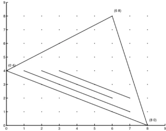
hulls of the sets{(0,2),(4,0),(11,0),(9,8)}and{(0,4),(8,0),(6,8)}
respec-tively (see Figures 3 and 4). The generic polynomials for this decomposition are as usual denotedgandh. The dominating edges of Newt(f) which allow
0 1 2 3 4 5 6 7 8 9 0 1 2 3 4 5 6 7 8 9 (0 4) (8 0) (6 8)
Figure 4: Newton polytope R of the generic polynomialh
a coprime edge factorisation are given by
δ1= conv{(0,6),(12,0)}, δ2= conv{(12,0),(19,0)}
and the corresponding edge polynomials are
fδ1
0 = y6+x2y5+x4y4+x8y2+x10y1+x12 fδ2
0 = x12+x19.
The coprime factors from which the lift begins are
gδ1
0 =y2+x2y+x4, hδ01 =y4+x8 gδ2
0 =x4+x11, hδ02 = 1.
The lifting process is then initiated; we refer the reader to our report [1] for more details. For now, we just note that the lines drawn in the interior of the polygons in Figures 3 and 4 indicate the first few layers of coefficients which are revealed during the lifting, and the lines in the interior of Newt(f) the
known coefficients of f which are used to do this. This choice for a partial
boundary factorisation is found to be successful leading to the specialisation of the 57 unknown coefficients of g and the 32 unknown coefficients of h.
The factors are
g = x4+x11+ (x2+x5+x10)y+y2+x9y8 h = x8+x7y+y4+x6y8.
which indeed satisfyf =gh.
It is perhaps appropriate at this stage to make a few observations on how sparse polynomials may be factored more quickly using Algorithm 10. Using
standard Hensel lifting the polynomial f above would first be randomised
to obtain a dense polynomial of total degree 31. It could have as many as (32×33)/2 = 528 non-zero terms, and heuristically around half this many
since f is over the binary field. The factor g we found above would then
correspond to a “dense” factor of our original polynomial of total degree 17. It would be found by Hensel lifting a degree 17 factor of the reduction modulo
yof our randomised version off, and (17×18)/2 = 153 terms (heuristically
half of them non-zero) need to be determined. In our algorithm, one restricts attention to unknown terms in possible factors whose exponents lie within certain polygons. Thus for the factorgwe found we only need to determine
57 coefficients. Moreover, if the polynomialf is sparse, there is good chance
that most of these term, and those inh, will be zero and so one can exploit
sparse data structures. The main benefit, though, of our approach appears to be for very sparse but composite polynomials of very high degree. In this case, one expects few coprime partial boundary decompositions, and as one can try and lift each one to a full factorisation, the algorithm will succeed (or fail) relatively quickly. If one randomises the polynomial by substitution of linear forms, the special sparse structure is completely lost. To factor the randomised polynomial using Hensel lifting, for example, one expects to have to try a large number of lifts. Thus, as demonstrated in the next section, our algorithm can be used to factor very sparse polynomials of degree beyond the reach of classical Hensel lifting.
8.2 Implementation
We have developed a preliminary implementation of the algorithm with the aim of demonstrating how it would work for bivariate polynomials overF2.
The work was carried out at the Oxford University Supercomputing Centre (OSC) on the Oswell machine, using an UltraSPARC III processor running at about 122 Mflop/s and with 2 GBytes of memory. The implementation was written using a combination of C and Magma programs, and was di-vided into three phases. In the first phase, the input polynomial is read and its Newton polytope computed using the asymptotically fast Graham’s al-gorithm for computing convex hulls [13]. In that phase we also compute all irredundant dominating sets, and output the edge polynomials. In the sec-ond phase, a Magma program invokes a univariate factorisation algorithm to perform the partial boundary factorisations, and the results are directed into the third phase program. In this last phase, a search for coprime dom-inating edges factorisations is performed, and when appropriate, the lifting process is started. The polynomial arithmetic was performed using classical
multiplication and division, and the triangular systems were solved using dense Gaussian elimination overF2.
We generated a number of random experiments with total degree reach-ing d = 2000. In all these cases, the input polynomial f was constructed
be multiplying two random polynomialsg and h of degree d/2 each with a
given number of non-zero terms. Specifically, for each polynomial the given number of exponent vectors (e1, e2) were chosen uniformly at random
sub-ject to 0≤e1+e2 ≤d/2. These vectors always included ones of the form
(e1,0), (0, e2) and (e3,(d/2)−e3) to ensure the polynomial was of the correct
degree and had no monomial factor. As the polynomials chosen were sparse the corresponding Newton polytopes had very few edges. In all these cases, the components of edge vectors of Newt(f) had a very small gcd, so that the
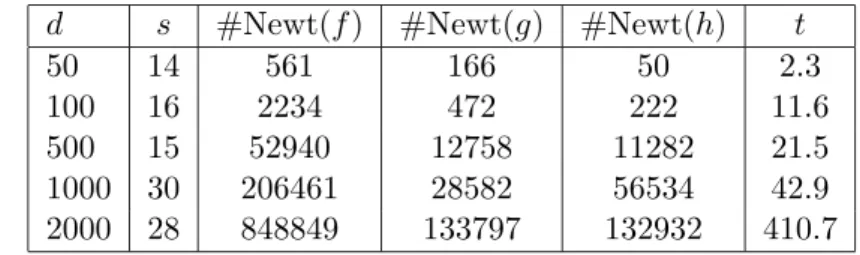
edges had few integral points and consequently the polygon itself had very few summands. The table below gives the running times (in seconds) of the total factorisation process to find at least one non-trivial factor involving all three phases described above. Here s is the number of non-zero terms of
the input polynomialf; #Newt(f), #Newt(g), and #Newt(h) are the total
number of lattice points in Newt(f), Newt(g) and Newt(h) respectively; and tis the total running time in seconds. The actual polynomialsf, g andh in
each of the five cases are also listed.
Table 1: Run time data for random experiments.
d s #Newt(f) #Newt(g) #Newt(h) t
50 14 561 166 50 2.3 100 16 2234 472 222 11.6 500 15 52940 12758 11282 21.5 1000 30 206461 28582 56534 42.9 2000 28 848849 133797 132932 410.7 d= 50: f =x9+x18y0+x22y8+x14y16+ (x4+x13)y20+ (x8+x17)y21+x18y24+ x17y28+x21y29+x1y32+y36+x4y37, g=x4+x13+x17y8+y16, h=x5+x1y16+y20+x4y21. d= 100: f =x26+x29y3+x31y5+x34y8+x20y13+x25y18+x6y19+(x9+x48)y22+ x53y27+y32+x28y41+x11y45+x14y48+x5y58+x33y67, g=x20+x25y5+y19+x5y45, h=x6+x9y3+x28y22+y13.
d= 500: f =x99+x151y30+x176y130+x151y142+x228y160+x99y181+x56y220+ x43y223+x108y250+x228y272+x176y311+x120y353+x108y362+x56y401+y443, g=x56+x108y30+x108y142+x56y181+y223, h=x43+x120y130+y220. d= 1000: f = x727+x678y3 +x935y13+x886y16+x679y67+x600y79+x887y80+ x551y82+x469y86+x420y89+x448y93+x399y96+x279y136+x636y143+x552y146+ x487y149+x421y153+x844y156+x400y160+x152y215+ (x21+x509)y222+ (1 + x378)y229+x357y236+x611y251+x562y254+x563y318+x163y387+x520y394, g=x448+x399y3+x400y67+y136+x357y143, h=x279+x487y13+x152y79+x21y86+y93+x163y251. d= 2000: f =x875+x856y6+x1469y18+x1450y24+x776y66+x1370y84+x722y157+ x703y163+x963y190+x944y196+x623y223+x864y256+x487y291+x468y297+ x647y334+x628y340+x982y375+x548y400+x235y514+x476y547+x769y619+ x1363y637+x0y648+x160y691+x616y776+x857y809+x381y910+x541y953, g=x487+x468y6+x388y66+y357+x381y619, h=x388+x982y18+x235y157+x476y190+x160y334+y291.
9
Conclusion
In this paper we have investigated a new approach for bivariate polynomial factorisation based on the study of their Newton polytopes. The approach combines results on polytopes with generalised Hensel lifting. In standard Hensel lifting, one lifts a factorisation from a single edge, and uniqueness can be ensured by randomising the polynomial to enforce coprimality condi-tions and make sure the edge being lifted from is sufficiently long. However, this randomisation is by substitution of linear forms which destroys the sparsity of the input polynomial. Our main theoretical contribution is to show how uniqueness may be ensured in the bivariate case, only under cer-tain coprimality conditions, and without restrictions on the lengths of the edges. For certain classes of sparse polynomials, namely those whose New-ton polytopes have few Minkowski decompositions, this gives a practical new approach which greatly improves upon Hensel lifting. As with Hensel lifting, our method has an exponential worst-case running time; however, we have demonstrated the practicality of our algorithm on several randomly chosen composite and sparse binary polynomials of high degree.
References
[1] F. Abu Salem, S. Gao, and A.G.B. Lauder “Factoring
poly-nomials via polytopes: extended version”, Internal Report, Oxford University Computing Laboratory.
Available from mid-January 2003 at:
http://web.comlab.ox.ac.uk/oucl/work/alan.lauder/
[2] E. R. Berlekamp, “Factoring polynomials over finite fields”, Bell
System Tech. J.,46(1967), 1853-1859.
[3] E. R. Berlekamp, “Factoring polynomials over large finite fields”,
Math. Comp.,24(1970), 713-735.
[4] D. G. Cantor and H. Zassenhaus“A new algorithm for factoring
polynomials over finite fields”,Math. Comp.36(1981), no. 154, 587– 592.
[5] A. L. Chistov, “An algorithm of polynomial complexity for
factor-ing polynomials, and determination of the components of a variety in a subexponential time” (Russian), Theory of the complexity of
computations, II., Zap. Nauchn. Sem. Leningrad. Otdel. Mat. Inst.
Steklov. (LOMI) 137 (1984), 124–188. [English translation: J. Sov.
Math.34(1986).]
[6] S. Gao, “Absolute irreducibility of polynomials via Newton
poly-topes,”J. of Algebra237(2001), 501–520.
[7] S. Gao, “Factoring multivariate polynomials via partial differential
equations,”Mathematics of Computation72 (2003), 801–822. [8] S. Gao and A.G.B. Lauder, “Decomposition of polytopes and
polynomials”,Discrete and Computational Geometry 26(2001), 89– 104.
[9] S. Gao and A.G.B. Lauder, Fast absolute irreducibility testing
via Newton polytopes, preprint 2003.
[10] S. Gao and A.G.B. Lauder, “Hensel lifting and bivariate
polyno-mial factorisation over finite fields”,Mathematics of Computation71
(2002), 1663-1676.
[11] J. von zur Gathen and E. Kaltofen, “Factoring sparse
[12] J. von zur Gathen and V. Shoup, “Computing Frobenius maps
and factoring polynomials”, Computational Complexity 2 (1992), 187–224.
[13] R. L. Graham, “An efficient algorithm for determining the convex
hull of a finite planar set”,Inform. Process. Lett. 1 (1972), 132-3. [14] D. Yu Grigoryev, “Factoring polynomials over a finite field and
solution of systems of algebraic equations” (Russian), Theory of the
complexity of computations, II., Zap. Nauchn. Sem. Leningrad.
Ot-del. Mat. Inst. Steklov. (LOMI)137(1984), 124–188. [English
trans-lation: J. Sov. Math. 34(1986).]
[15] M. van Hoeij, “Factoring polynomials and the knapsack problem,”
J. Number Theory95(2002), 167–189.
[16] E. Kaltofen, “Polynomial-time reductions from multivariate to
bi-and univariate integral polynomial factorisation”, SIAM J. Comp., vol. 14, 469-489, 1985.
[17] E. Kaltofen and V. Shoup, “Subquadratic-time factoring of
poly-nomials over finite fields”, Math. Comp. 67 (1998), no. 223, 1179– 1197.
[18] E. Kaltofen and B. Trager, “Computing with polynomials given
by black boxes for their evaluations: Greatest common divisors, fac-torization, separation of numerators and denominators”,J. Symbolic
Comput.9 (1990), 301-320.
[19] A. K. Lenstra, “Factoring multivariate integral polynomials”,
The-oret. Comput. Sci.34(1984), no. 1-2, 207–213.
[20] A. K. Lenstra, “Factoring multivariate polynomials over finite
fields”,J. Comput. System Sci. 30(1985), no. 2, 235–248.
[21] A. K. Lenstra, “Factoring multivariate polynomials over algebraic
number fields”,SIAM J. Comput.16(1987), no. 3, 591–598.
[22] A. K. Lenstra, H.W. Lenstra, Jr. and L. Lov´asz, “Factoring
polynomials with rational coefficients”,Mathematische Annalen,161
(1982), 515–534.
[23] D.R. Musser, “Multivariate polynomial factorization”,J. ACM 22
[24] D. Wan, “Factoring polynomials over large finite fields”, Math.
Comp.54(1990), No. 190, 755–770.
[25] P. S. Wang, “An improved multivariate polynomial factorization
algorithm”,Math. Comp.32(1978), 1215–1231.
[26] P. S. Wang and L. P. Rothschild, “Factoring multivariate
poly-nomials over the integers,”Math. Comp.29(1975), 935–950. [27] H. Zassenhaus, “On Hensel factorization I”, J. Number Theory 1