Nonparametric estimation of the conditional tail index and extreme quantiles under random censoring

(1)

Nonparametric estimation of the conditional tail index

and extreme quantiles under random censoring

Path´

e Ndao, Aliou Diop, Jean-Fran¸cois Dupuy

To cite this version:

Path´

e Ndao, Aliou Diop, Jean-Fran¸cois Dupuy. Nonparametric estimation of the conditional

tail index and extreme quantiles under random censoring. Computational Statistics and Data

Analysis, Elsevier, 2014, 79, pp.63-79.

<

10.1016/j.csda.2014.05.007

>

.

<

hal-00802804

>

HAL Id: hal-00802804

https://hal.archives-ouvertes.fr/hal-00802804

Submitted on 20 Mar 2013

HAL

is a multi-disciplinary open access

archive for the deposit and dissemination of

sci-entific research documents, whether they are

pub-lished or not.

The documents may come from

teaching and research institutions in France or

abroad, or from public or private research centers.

L’archive ouverte pluridisciplinaire

HAL

, est

destin´

ee au d´

epˆ

ot et `

a la diffusion de documents

scientifiques de niveau recherche, publi´

es ou non,

´

emanant des ´

etablissements d’enseignement et de

recherche fran¸cais ou ´

etrangers, des laboratoires

publics ou priv´

es.

(2)

Nonparametric estimation of the conditional tail

index and extreme quantiles under random

cen-soring

Path ´e NDAO

LERSTAD, Universit é Gaston Berger, Saint Louis, S én égal. Email: [email protected]

Aliou DIOP

LERSTAD, Universit é Gaston Berger, Saint Louis, S én égal. Email: [email protected]

Jean-Franc¸ois DUPUY†

IRMAR-Institut National des Sciences Appliqu ´ees de Rennes, France. Email: [email protected]

Abstract. In this paper, we investigate the estimation of the tail index and extreme quantiles of a heavy-tailed distribution when some covariate information is avail-able and the data are randomly right-censored. We construct several estimators by combining a moving-window technique (for tackling the covariate information) and the inverse probability-of-censoring weighting method, and we establish their asymptotic normality. A comprehensive simulation study is conducted to evalu-ate the finite-sample performance of the proposed estimators and to identify their application scope.

Keywords: Random censoring, conditional extreme value index, condi-tional extreme quantiles, heavy-tailed distribution, moving window, simulations.

1. Introduction

LetY1, . . . , Ynbe a sequence of independent and identically distributed replicates

of a random variable Y. One question of great practical interest in many do-mains (reliability, hydrology, insurance, meteorology. . . ) is to estimate extreme quantiles of the distribution ofY that is, quantities of the form

F←(1−α) = inf{y:F(y)≥1−α}

where α is so small that this quantile falls beyond the range of the observed dataY1, . . . , Yn. This problem has been widely investigated so far. It involves the

(3)

estimation of the so-called extreme value index (or tail index)γ. This parameter drives the tail heaviness of the distribution ofY and thus plays a central role in the analysis of extremes, making its estimation a crucial issue. Detailed accounts on extreme value theory (and in particular on the estimation of the extreme value index and extreme quantiles) can be found, for example, in [2, 9, 14]. Here, we consider the situation where some covariate information X is available to the investigator, and the distribution ofY depends on X. Then for every X =x, we consider the problem of estimating the conditional extreme value indexγ(x) and conditional extreme quantilesF←(1−α|x) = inf{y:F(y|x)≥1−α}of the distributionF(·|x) ofY givenx. Several papers already address the estimation of the conditional extreme value index and conditional extreme quantiles (see for example [10, 11, 13] and the references therein). In the present paper, we consider these issues in the more complicated situation where the observationsY1, . . . , Yn

are randomly right-censored. Censoring occurs for example in the statistical analysis of event time data, whereY represents the time elapsed from some time origin until the occurrence of some event of interest (death of a patient, ruin of a company. . . ) andX represents some available covariate information (biological markers recorded on a patient, economic characteristics of a company. . . ). If censoring is present, the observations consist of triplets (Zi, δi, Xi),i= 1, . . . , n,

whereZi= min(Yi, Ci),δi= 1{Yi≤Ci}, 1{·}is the indicator function, andCiis a

random censoring time for thei-th individual, that provides a lower bound onYi

ifδi= 0. The estimation of the extreme value index and extreme quantiles from

censored data has been considered, among others, by [3, 5, 8, 12] when there is no covariate informationX. Here, we consider the estimation of these quantities when both censoring and covariate information are present.

We first construct several estimators of the conditional tail indexγ(x) of the distribution of Y given x, and we establish their asymptotic normality. Our construction combines a moving-window approach (such as developped in [10] in the uncensored case) with the inverse probability-of-censoring weighting (IPCW) principle (such as used in [8] for estimating the unconditional extreme value index with censoring). Then, we construct Weissman-type estimators of the conditional extreme quantile F←₍₁₋_α_|_{x) under censoring. We establish the} asymptotic normality of the proposed estimators. Finally, we conduct a simu-lation study to evaluate the finite-sample performance of all these estimators. The rest of the paper is organized as follows. In Section 2, we set the model and some useful notations. The proposed estimators are constructed in Section 3. In Section 4, we investigate their asymptotic properties. The proofs are postponed to the appendix. The results of a comprehensive simulation study are reported in Section 5. A discussion and some perspectives conclude the paper.

2. Model and notations

Let (Y1, . . . , Yn) ben independent copies of a non-negative random variableY

(4)

covariate X ∈ X, where X denotes a compact set in Rp. We assume that

each Yi can be right-censored by a non-negative random variable Ci (the Ci’s

are defined on the same probability space (Ω,C,_P) as theYi’s, and are assumed

independent of each other), such that we really observe thenindependent triplets (Zi, δi, xi), i= 1, . . . , n, whereZi = min(Yi, Ci) andδi= 1{Yi≤Ci}. YiandCiare

assumed to be independent. In the sequel,dwill denote the Euclidean distance onRp, and →D will denote the convergence in distribution.

For everyx∈ X, we denote byF(·|x) andG(·|x) respectively the conditional cumulative distribution functions ofY andCgivenX =x. We assume that for every x ∈ X, F(·|x) and G(·|x) belong to the domain of attraction of Fr´echet distributions with shapesγ1(x) andγ2(x) respectively. This implies thatF(·|x) andG(·|x) can be written as

F(u|x) = 1−u−1/γ1(x)_L

1(u, x) and G(u|x) = 1−u−1/γ2(x)L2(u, x), whereγ1(·) andγ2(·) are unknown positive functions of the covariatex(referred to as conditional tail index functions), and for everyx∈ X,L1(·, x) andL2(·, x) are slowly varying at infinity that is, for everyλ >0,

Li(λu, x)/Li(u, x)−→1 as u−→ ∞, i= 1,2.

Note that by independence ofY andC, the conditional cumulative distribution functionH(·|x) ofZ givenX =xis also heavy-tailed, with conditional extreme value indexγ(x) =γ1(x)γ2(x)/(γ1(x) +γ2(x)). To see this, note that for every uandx,

1−H(u|x) = (1−F(u|x))(1−G(u|x))

= u−1/γ1(x)_{L1(u, x)u}−1/γ2(x)_{L2(u, x)}

= u−1/γ(x)L(u, x)

whereγ(x) is as above andL(u, x) =L1(u, x)L2(u, x). Moreover, lim u→∞ L(λu, x) L(u, x) = limu→∞ L1(λu, x) L1(u, x) L2(λu, x) L2(u, x) = 1.

Finally, let q(α, x) be the conditional quantile of order 1 −α (α ∈ (0,1)) of F(·|x), defined by F(q(α, x)|x) = 1−α. Given a sample of observations (Z1, δ1, x1), . . . ,(Zn, δn, xn), our aims are to build and evaluate pointwise

es-timators of the conditional tail index function γ1(x) and conditional extreme quantilesq(α, x).

3. The proposed estimators

Several estimators have been proposed for the extreme value index and extreme quantiles when either some covariate information is available or theYi’s are

(5)

these quantities by combining a moving-window approach (proposed in [10] for estimating the conditional tail index function without censoring) with the IPCW principle (used for example in [8] for estimating the extreme value index in a model without covariate, see also [5]). We first construct a pointwise estimator of the conditional tail index functionγ1(x).

3.1. Estimation of the conditional tail index function

Ifx∈ X andr >0, letB(x, r) denote the ball in_Rp _{with center}_x_{and radius}_r

that is,B(x, r) ={t∈Rp, d(x, t)≤r}. Lethn,xbe a positive sequence tending

to 0 asntends to infinity, and definemn,x:=P n

i=11{xi∈B(x,hn,x)} (respectively

φ(hn,x) :=n−1mn,x) as the number (respectively the proportion) of the

obser-vations (Zi, xi) lying in [0,∞)×B(x, hn,x). Let Z(1)x ≤ . . . ≤ Z

x

(mn,x) be the

ordered values of Z for these observations, and let δ₍₁₎x , . . . , δ₍x_m

n,x) be the

cor-respondingδ’s (that is,δx

(i)=δj ifZ(xi)=Zj). Note that since X is controlled,

mn,xandφ(hn,x) are nonrandom numbers. If theZ(xi)were not censored, Gardes and Girard (see [10]) propose to estimate γ1(x) by a Hill-type estimator of the form b γ_k(H) x,mn,x(x) :=M (1) kx,mn,x:= 1 kx kx X i=1 ilog Zx (mn,x−i+1) Zx (mn,x−i) ! (3.1)

where kx is a sequence of integers such that 1 ≤ kx ≤ mn,x. Several other

estimators of the extreme value index can be adapted to the situation whereγ1 is a function of a covariate. For example, one may consider the following adapted version of the moment estimator:

b γ_k(M) x,mn,x(x) :=M (1) kx,mn,x+ 1− 1 2  1− (M_k(1) x,mn,x) 2 M_k(2) x,mn,x   −1 (3.2) where M_k(2) x,mn,x := 1 kx kx X i=1 ilog Z x (mn,x−i+1) Zx (mn,x−i) !!2 ,

or the following adapted version of the UH estimator:

b γ_k(U H) x,mn,x(x) := 1 kx kx X i=1 log   Z₍x_m n,x−i)bγ (H) i,mn,x(x) Zx (mn,x−kx)bγ (H) kx,mn,x(x)  . (3.3)

The estimators (3.2) and (3.3) extend the estimators proposed in [7] and [4] respectively when there is no covariate information. In what follows, we adapt the estimators (3.1), (3.2), and (3.3) to the case where censoring occurs (note

(6)

that these estimators are not consistent forγ1(x) if they are directly applied to the sample (Zi, δi, xi), i= 1, . . . , n. Indeed, they will converge to the extreme

value indexγ(x) of the conditional distribution ofZ).

To accomodate censoring, we divide the estimators (3.1), (3.2), and (3.3) by the proportion b px= 1 kx kx X i=1 δ₍x_m n,x−i+1)

of uncensored observations among the kx largest Z’s in a neighbourhood of x

(a similar idea was used, for example, in [5] and [8] for estimating the extreme value index without covariate). For allx∈ X, our proposal is thus to estimate γ1(x) by b γ_k(c,.) x,mn,x(x) := b γ_k(.) x,mn,x(x) b px (3.4) where the· in γ_b_k(c,.) x,mn,x(x) andγb (.)

kx,mn,x(x) stands for any of the Hill, moment,

and UH estimator.

3.2. Estimation of conditional extreme quantiles

In this section, we further address the estimation of conditional extreme quantiles q(αmn,x, x)∈Rof order 1−αmn,x of the distribution of Y given X =x. Such

quantiles verify 1−F(q(αmn,x, x)|x) =αmn,x whereαmn,x→0 asmn,x→+∞.

For everyx∈ X, we first consider the following conditional Kaplan-Meier-type estimator, based on the moving-window approach described in the section 3.1:

1−Fbmn,x(y|x) = mn,x Y i=1 _m n,x−i mn,x−i+ 1 δ(i)x 1{Zx_(i)≤y} .

Based on this, we propose to estimate q(αmn,x, x) by the following

Weissman-type estimator ([15]): b q(c,.)(αmn,x, x) =Z x (mn,x−kx) 1−Fbmn,x(Z x (mn,x−kx)|x) αmn,x !bγ (c,.) kx,mn,x(x) (3.5) where _bγ_k(c,.)

x,mn,x(x) is any of the estimators (3.4). Note that (3.5) extends the

conditional extreme quantile estimator proposed in [13] in the situation where there is no censoring.

In the next section, we establish the asymptotic properties of our estimators (3.4) and (3.5).

(7)

4. Asymptotic results

We first state some regularity conditions that will be needed for proving our asymptotic results (these conditions are used in [10] to prove the asymptotic normality of the conditional tail index estimator without censoring, see also [5] for the case with censoring but no covariate information). We assume that:

C1 for everyx∈ X, the conditional distribution functionsF(·|x) andG(·|x) are absolutely continuous,

C2 for every x∈ X, there exists a function ρ(x)< 0 and a regularly varying functionb(·, x) with index ρ(x) such that for anyu >0,

lim t→∞ H← 1− 1 tu |x /H← 1−1 t |x −uγ(x) b(t, x) =u γ(x)uρ(x)−1 ρ(x) , The following assumptions are also required (they are similar to the conditions given in [5] for estimating the unconditional extreme value index with censoring). For any x ∈ X, let px = γ2(x)/(γ1(x) +γ2(x)). Assume that as n −→ ∞,

kx−→ ∞, _mkx n,x −→0, and: C3 √kxb _m n,x kx , x −→λ(x)<∞, C4 √1 kx Pkx i=1 h px H←1− i mn,x |x −px i −→(x)<∞, C5 letting A(s, t) :={1− kx mn,x ≤ t < 1,|t−s| ≤ C √ kx mn,x, s < 1}, we assume √ kx sup A(s,t) |px(H←(t|x))−px(H←(s|x))| −→0, for allC >0.

We are now in position to state our first main result. Its proof is given in the appendix.

Theorem 4.1. Letx∈ X. Assume that the conditions C1-C5 hold and that there exist some functionsm(·)andσ(·)such that√kx

b γ_k(.) x,mn,x(x)−γ(x) _D −→ N m(x)λ(x), σ2(x). Then the following holds:

p kx b γ_k(c,.) x,mn,x(x)−γ1(x) D −→ N 1 px (λ(x)m(x)−γ1(x)(x)),σ 2_{(x) +}_γ1(x)2_p x(1−px) p2 x .

Considering successively each of the Hill, moment, and UH estimator, we obtain the following corollary:

(8)

Corollary 4.2. Under the assumptions of Theorem 4.1, the following holds for everyx∈ X: p kx b γ_k(c,H) x,mn,x(x)−γ1(x) D −→ N ₋_γ 1(x)(x) px + λ(x) px(1−ρ(x)) ,γ 3 1(x) γ(x) , p kx b γ_k(c,U H) x,mn,x(x)−γ1(x) D −→ N −γ1(x)(x) px + λ(x) px(1−ρ(x)) ,γ 2 1(x) γ2_(x)(1 +γ1(x)γ(x)) , p kx b γ_k(c,M) x,mn,x(x)−γ1(x) D −→ N ₋_γ1(x)(x) px + λ(x) px(1−ρ(x)) ,γ 2 1(x) γ2_(x)(1 +γ1(x)γ(x)) .

This corollary is easily proved by noting that m(x) = (1−ρ(x))−1 (for all γ_k(H)

x,mn,x(x),γ

M

kx,mn,x(x), andγ

(U H)

kx,mn,x(x)), and that (see [1] and [7]):

σ2(x) =      γ2_{(x) for}_γ(H) kx,mn,x(x) 1 +γ2_{(x) for}_γ(M) kx,mn,x(x) 1 +γ2_{(x) for}_γ(U H) kx,mn,x(x).

We now turn to the asymptotic properties of the estimator (3.5) of the con-ditional extreme quantiles. The following adcon-ditional notations and regularity condition are needed (see [13]):

C6 for every x∈ X, the conditional quantile function α∈ (0,1) 7→ q(α, x)∈

(0,+∞) is differentiable and the functionα∈(0,1)7→∆(α, x) =γ1(x) + α(∂logq(α, x)/∂αis continuous and tends to 0 asαtends to 0.

Let ∆(a, x) = sup_α_∈(0_,a₎|∆(α, x)|and for anya∈(0,1/2), let

ωn(a) = sup log q(α, t) q(α, t0₎ ;α∈(a,1−a),(t, t0)∈(B(x, hn,x))2 .

We now state our second main result, which gives the asymptotic properties of the estimator (3.5) (its proof is given in the appendix).

Theorem 4.3. Assume that the conditions C1-C6 hold. Let (βmn,x)n≥1:=

(1−Fbmn,x(Z

x

(mn,x−kx)|x))n≥1 and(αmn,x)n≥1 be a sequence such thatαmn,x <

βmn,x. Let also ξmn,x = (mn,xβmn,x)

1/2_log _β

mn,x/αmn,x

. Assume that as n → ∞, there exists δ > 0 such that (mn,xβmn,x)

2_ω

n(m−(1+ δ)

(9)

k1x/2max{ξm−1n,x,∆(βmn,x, x)} →0. Then √ kx log(βmn,x/αmn,x) log qb (c,.)_(α mn,x, x) q(αmn,x, x) ! D −→ N ₁ px (λ(x)m(x)−γ1(x)(x)), σ2_{(x) +}_γ1(x)2_p x(1−px) p2 x .

From this, one can easily derive the asymptotic distribution of q_b(c,.)_(α

mn,x, x)

for each particular case (Hill, moment, UH). This proceeds along the same lines as the Corollary 4.2, and is omitted for conciseness.

5. Simulation study

In this section, we conduct a comprehensive simulation study to evaluate the performance of the proposed estimators (3.4) and (3.5) of the conditional extreme value index and conditional quantiles. We investigate both the accuracy of these estimators and the quality of the Gaussian approximation of their asymptotic distributions. We identify the application scope of each of these estimators (in terms of the sample size and censoring proportion).

5.1. The study design

The simulation design (inspired by [13]) is as follows. We simulate R = 1000 samples of sizen(n= 500,1000,1500,2000) of independent replicates (Zi, δi, xi),

whereZi= min(Yi, Ci) andxi ∈[0,1]. The conditional distribution ofYi given

X =xi is Pareto with parameter

γ1(x) =.5 (.1 + sin(πx))

1.1−.5 exp−64 (x−.5)2

and the distribution of Ci is Pareto with a parameter γ2 chosen to yield the

desired censoring percentagec(cis successively chosen equal to 10%,25%,40%). The pattern ofγ1(·) is given on Figure 1.

FIGURE 1 HERE

For each of theRsamples, we estimateγ1(·) atx= 0.5 (γ1(0.5) = 0.35) by each of the Hill, moment, and UH estimators (3.4). The moving window approach described in Section 3 is used with the ball B(0.5,0.1). Choosing the most appropriate value for kx is a difficult issue, and we refer the reader to [6] and

[13] for a detailed discussion. A more detailed investigation of this issue in our setting falls out of the scope of the present paper. For illustrative purpose, let γ_b_i,m(c,.),j

n,x(x) denote the estimate of γ1(x) obtained in the j-th sample (j =

(10)

kx: kxopt:= argmin 1≤i≤mn,x M SE(_bγ_i,m(c,.) n,x(x)) = argmin 1≤i≤mn,x R−1PR j=1(bγ (c,.),j i,mn,x(x)−γ1(x)) 2

(where MSE stands for mean square error), keeping in mind that this method should be modified in practice sinceγ1(x) is unknown. Using this value ofkx, we

calculate, for each of the Hill, moment, and UH estimators and each censoring percentage, the averaged estimates of γ1(x), along with their empirical root mean square and mean absolute errors. Finally, for each configuration of the simulation design parameters, we compute confidence intervals of asymptotic level 95% forγ1(x), and we obtain the empirical coverage probabilities over the R intervals (plug-in estimates are obtained for the asymptotic variance). The results are given in Table 1.

TABLE 1 HERE

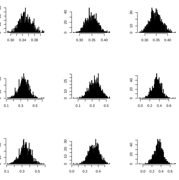
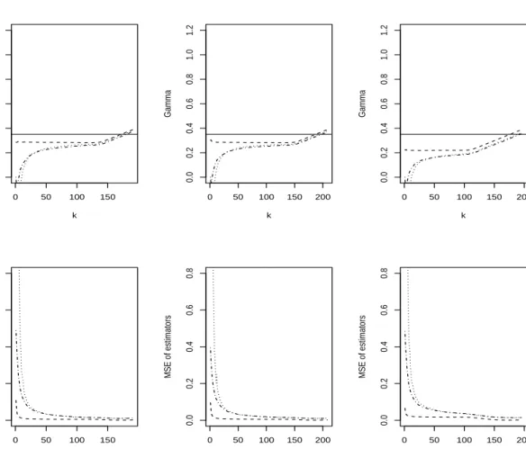
In order to evaluate the quality of the Gaussian approximation of the asymptotic distribution of the proposed estimator (3.4) of the conditional tail index (at x= 0.5), we plot the histograms of theRHill, moment, and UH estimates. The histograms are given in the Figures 2 (for n= 500) and 3 (forn= 1500). For each of Hill, moment and UH, we also represent the averaged estimate ofγ1(x) and the corresponding empirical MSE, as functions of kx (see Figure 4). The

plots are given for c= 10%,25%,40% and n= 1000 (the graphs for the other values ofnyield similar observations and are therefore omitted).

FIGURES 2, 3, and 4 HERE

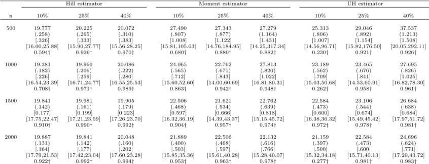
Next, we turn to the estimation of the extreme quantile q(1/5000,0.5) of order 1−1/5000 of the conditional distribution of Y given x = 0.5 (q(1/ 5000,0.5)≈19.70786). For each configuration of the simulation design parame-ters, we calculate the conditional estimate (3.5), based on the Hill, moment, and UH estimators of the conditional tail index. Then, for each sample size nand censoring percentagec, we obtain the averaged value of theq_b(c,.),j_(1/5000,_0.5)

(j= 1, . . . , R), along with their empirical root mean square and mean absolute errors. Finally, we compute confidence intervals (with asymptotic level 95%) forq(1/5000,0.5) and we obtain the empirical coverage probabilities over theR resulting intervals. Table 2 reports the results.

TABLE 2 HERE

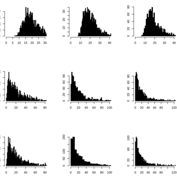
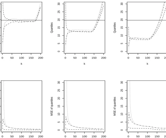
Similarly as above, we evaluate the quality of the Gaussian approximation of the asymptotic distribution of the estimator (3.5) of the extreme quantileq(1/ 5000,0.5). We plot the histograms of the R= 1000 estimates of q(1/5000,0.5) (based on the Hill, moment, and UH estimates of the conditional tail index). The histograms are given in the Figures 5 (n = 500) and 6 (n = 1500). We also represent the averaged estimate of q(1/5000,0.5) and the corresponding empirical MSE as functions ofkx(see Figure 7), when the conditional tail index

is estimated by the Hill, moment, and UH estimators respectively. The plots are given forc = 10%,25%,40% andn= 1000 (the graphs for n= 500,1500,2000 yield similar observations and are therefore omitted).

(11)

FIGURES 5, 6, and 7 HERE

5.2. Results

From the Table 1, the quality of the various considered estimators ofγ1(x) degra-dates as the censoring percentage increases and the sample size decreases. Note that the empirical coverage probabilities increase as the censoring proportion in-creases, which comes from the fact that the variance estimate increases (this in turn implies that the confidence intervals become wider, and not more precise). The Hill estimator performs much better than the moment and UH for every configuration of the simulation parameters. In particular, the Hill estimator is much less biased than the two others (this is particularly noticeable when the sample size is moderate) and is more robust to censoring. The Figures 2 and 3 reveal that the Gaussian approximation of the asymptotic distribution of the Hill estimator is reasonably satisfied even for a moderate sample size (n= 500). Whenn= 500 and the censoring percentage is moderate (25%) to large (40%), the distributions of the moment and UH estimators are slightly skewed. The superiority of the Hill estimator is also noticeable on the Figure 4.

From the Table 2, the moment and UH estimators of the conditional extreme quantile appear to be biased, even when the sample size is large, and much less robust to censoring than the Hill-based estimator. From this table also, the Hill estimator provides a satisfactory approximation of the true extreme quantile, even when the censoring is heavy and the sample size is small. Moreover, the moment and UH estimators of the conditional extreme quantile suffer numerical instability, as can be noticed from the upper bounds of the confidence inter-vals, which can be meaningless when the sample size is moderate (n = 500) or the censoring fraction is moderate to large. From the Figures 5 and 6, the moment and UH estimators are strongly skewed in almost all configurations of the simulation design. They appear to be moderately skewed when the sample size is large and the censoring proportion is small (10%). The Hill estimator is moderately skewed when the sample size is small. Its distribution is close to the Gaussian when the sample size is large. Finally, from the Figure 7, we observe that the quantile estimate is rather sensitive to the choice ofkx unless

the censoring fraction is small. From this figure, we also observe the superiority of the Hill estimator over the moment and UH in terms of MSE.

6. Discussion and perspectives

In this paper, we have considered the estimation of the tail index and extreme quantiles of a heavy-tailed distribution when some covariate information is avail-able and the data are randomly right-censored. We have constructed several estimators for these quantities, by combining a moving-window approach and the inverse probability-of-censoring weighting method. We have established the asymptotic normality of these estimators. A comprehensive simulation study

(12)

was conducted to evaluate and compare their finite-sample performance. The Hill estimators of the conditional tail index and extreme quantiles appear to outperform the moment and UH estimators: the Hill estimators are less biased, more robust to censoring and more stable with respect to the choice ofkx.

Several issues still deserve attention. In particular, the proposed estimators rely on the smoothing parameterhn,x and the numberkx of upper order

statis-tics. A detailed investigation of how one may choose these values in practice is needed, and is the topic for future research. In this work, we considered the case where the covariateX is controlled. The case where X is random is the topic for our current investigations.

Appendix: proofs of theorems

Proof of Theorem 4.1. The proof proceeds along the same lines as the proof of Theorem 1 in [8], thus we mention the main steps only. We consider first the following decomposition (for any of the Hill, moment, and UH estimator):

p kx b γ_k(c,.) x,mn,x(x)−γ1(x) = 1 b px p kx b γ_k(.) x,mn,x(x)−γ(x) +1 b px p kx(γ(x)−γ1(x)pbx) = 1 b px p kx b γ_k(.) x,mn,x(x)−γ(x) (6.6) −γ1(x) b px p kx b px− γ2(x) γ1(x) +γ2(x) . Consider first the first term in the right-hand side of (6.6). Under the conditions stated in Section 4, it follows from [10] that asn→ ∞,

p kx b γ_k(.) x,mn,x(x)−γ(x) _D −→ N m(x)λ(x), σ2(x) .

Moreover, for everyx∈ X, √kx(pbx−px)

D

−→ N((x), px(1−px)) (the proof is

similar to the proof of Theorem 1 in [8] and is therefore omitted) and thus

√ kx b px b γ(_k.) x,mn,x(x)−γ(x) _D −→ N _m(x)λ(x) px ,σ 2_(x) p2 x .

Consider now the second term in the right-hand side of (6.6). As mentioned above,√kx(pbx−px)

D

−→ N ((x), px(1−px)), and thus by independence, p kx b γ_k(c,.) x,mn,x(x)−γ1(x) D −→ N ₁ px (λ(x)m(x)−γ1(x)(x)),σ 2_{(x) +}_γ1(x)2_p x(1−px) p2 x .

(13)

Proof of theorem 4.3. The proof follows the same steps as the proof of Theorem 4.3.3 in [13], hence we only outline the main steps. Letting βmn,x :=

1−Fbmn,x(Z x (mn,x−kx)|x), we get that βmn,x = mn,x−kx Y i=1 _m n,x−i mn,x−i+ 1 δ(i)x ≤1. Moreover, kx mn,x = mn,x−kx Y i=1 _m n,x−i mn,x−i+ 1 ≤βmn,x.

It follows that kx ≤mn,xβmn,x ≤mn,x and thus,mn,xβmn,x → ∞ as n→ ∞.

The Theorem 4.3.1 of [13] therefore applies, and together with the delta-method, it implies that mn,xβmn,x 1/2 log Zx (mn,x−kx) q(βmn,x, x) ! =Op(1). (6.7)

Now, it follows from (3.5) that

log_bq(c,.)(αmn,x, x) = logZ x (mn,x−kx)+bγ (c,.) kx,mn,x(x) log _β mn,x αmn,x and thus √ kx log(βmn,x/αmn,x) log qb (c,.)_(α mn,x, x) q(αmnx, x) ! = √ kx log(βmn,x/αmn,x) log Z x (mn,x−kx) q(βmn,x, x) ! +pkx b γ_k(c,.) x,mn,x(x)−γ1(x) − √ kx log(βmn,x/αmn,x) log q αmn,x, x q(βmn,x, x) ! +γ1(x) log _β mn,x αmn,x ! :=ξ1,mn,x+ξ2,mn,x−ξ3,mn,x

(14)

where ξ1,mn,x = √ kx log(βmn,x/αmn,x) log Zx (mn,x−kx) q(βmn,x, x) ! ξ2,mn,x = p kx b γ_k(c,.) x,mn,x(x)−γ1(x) ξ3,mn,x = √ kx log(βmn,x/αmn,x) log q αmn,x, x q(βmn,x, x) ! +γ1(x) log _β mn,x αmn,x ! .

Note first that with the notations of Theorem 4.3,

ξ1,mn,x= p kxξ−1mn,x(mn,xβmn,x) 1/2_log Z x (mn,x−kx) q(βmn,x, x) ! .

It follows from (6.7) and the assumptions of Theorem 4.3 that ξ1,mn,x → 0

in probability as n → ∞. Next, from the Theorem (4.1), ξ2,mn,x converges

in distribution to N1 px(λ(x)m(x)−γ1(x)(x)), σ2₍_x₎₊_γ2 1(x)px(1−px) p2 x . Finally, some calculations yield

ξ3,mn,x=− √ kx log(βmn,x/αmn,x) Z βmn,x αmn,x ∆(u, x) u du. By bounding ∆(u, x) above, we obtain that|ξ3,mn,x| ≤k

1/2

x ∆(βmn,x, x) and thus,

ξ3,mn,x → 0 in probability as n → ∞ under the assumptions of Theorem 4.3.

Finally, √ kx log(βmn,x/αmn,x) log qb (c,.)_(α mn,x, x) q(αmnx, x) ! :=ξ1,mn,x+ξ2,mn,x−ξ3,mn,x converges in distribution toN1 px(λ(x)m(x)−γ1(x)(x)), σ2(x)+γ2₁(x)px(1−px) p2 x asn→ ∞. References

[1] J. Beirlant, G. Dierckx, and A. Guillou. Estimation of the extreme-value index and generalized quantile plots. Bernoulli, 11(6):949–970, 2005. [2] J. Beirlant, Y. Goegebeur, J. Teugels, and J. Segers. Statistics of extremes.

Wiley, 2004.

[3] J. Beirlant, A. Guillou, G. Dierckx, and A. Fils-Villetard. Estimation of the extreme value index and extreme quantiles under random censoring. Extremes, 10(3):151–174, 2007.

(15)

[4] J. Beirlant, P. Vynckier, and J. L. Teugels. Tail index estimation, Pareto quantile plots, and regression diagnostics. J. Amer. Statist. Assoc., 91(436):1659–1667, 1996.

[5] B. Brahimi, D. Meraghni, and A. Necir. On the asymptotic normality of Hill’s estimator of the tail index under random censoring. ArXiv e-prints, February 2013.

[6] L. de Haan and L. Peng. Camparison of tail index estimators. Statistica Neerlandica, 52 (1):60–70, 1998.

[7] A. L. M. Dekkers, J. H. J. Einmahl, and L. de Haan. A moment estimator for the index of an extreme-value distribution. Ann. Statist., 17(4):1833–1855, 1989.

[8] J. H. J. Einmahl, A. Fils-Villetard, and A. Guillou. Statistics of extremes under random censoring. Bernoulli, 14(1):207–227, 2008.

[9] P. Embrechts, C. Kl¨uppelberg, and T. Mikosch. Modelling extremal events. Springer, 1997.

[10] L. Gardes and S. Girard. A moving window approach for nonparametric estimation of the conditional tail index.J. Multivariate Anal., 99(10):2368– 2388, 2008.

[11] L. Gardes and S. Girard. Conditional extremes from heavy-tailed distri-butions: an application to the estimation of extreme rainfall return levels. Extremes, 13(2):177–204, 2010.

[12] M. I. Gomes and M. M. Neves. A note on statistics of extremes for censoring schemes on a heavy right tail.In Luzar-Stiffler, V., Jarec, I. and Bekic, Z. (eds.), Proceedings of ITI 2010, SRCE Univ. Computing Centre Editions, pages 539–544, 2010.

[13] A. Lekina. Estimation non-paramétrique des quantiles extrêmes condition-nels. Thèse de doctorat, Université de Grenoble, 2010.

[14] R.-D. Reiss and M. Thomas. Statistical analysis of extreme values with applications to insurance, finance, hydrology and other fields. Birkh¨auser, 2007.

[15] I. Weissman. Estimation of parameters and large quantiles based on thek largest observations. J. Amer. Statist. Assoc., 73:812–815, 1978.

(16)

Hill estimator Moment estimator UH estimator n 10% 25% 40% 10% 25% 40% 10% 25% 40% 500 .349 .350 .345 .323 .315 .317 .322 .304 .323 (.037) (.043) (.045) (.116) (.134) (.172) (.114) (.137) (.171) [.030] [.034] [.035] [.090] [.107] [.136] [.090] [.109] [.135] [.273,.425 ] [.270,.428] [.256,.434] [.081,.566] [.040,.591] [0∗,.652] [.084,.561] [.029,.580] [0∗,.652] .758† .961† .963† .900† .908† .950† .945† .960† .964† 1000 .346 .349 .346 .337 .330 .334 .339 .336 .326 (.027) (.029) (.032) (.081) (.097) (.119) (.081) (.099) (.119) [.022] [.023] [.026] [.065] [.076] [.093] [ .065] [.079] [.093] [.293,.400] [.290,.408] [.283,.409] [.166,.509] [.124,.535] [.095,.572] [.171,.508] [.135,.536] [.088,.561] .969† .986† .990† .959† .964† .970† .965† .968† .970† 1500 .347 .348 .345 .344 .339 .335 .342 .340 .339 (.021) (.025) (.030) (.067) (.071) (.101) (.067) (.072) (.101) [.017] [.020] [.024] [.053] [.057] [.080] [.053] [.058] [.081] [.304,.389] [.300, .396] [.289,.401] [.208,.480] [.171,.506] [.122,.549] [.206,.477] [.183,.511] [.129,.551] .973† .993† .995† .971† .977† .981† .975† .980† .984† 2000 .349 .349 .348 .337 .340 .335 .342 .345 .337 (.019) (.020) (.022) (.058) (.067) (.087) (.058) (.068) (.087) [.015] [ .016] [ .017] [.045] [.052] [.068] [.046] [.053] [.068] [.311,.387] [.310,.389] [.303,.394] [.212,.463] [.202,.477] [.160,.509] [.219,.466] [.209,.480] [.164,.512] .987† .995† .998† .980† .984† .986† .981† .984† .987†

Table 1 (simulation results forγ1(x)). For each configuration of the simulation parameters (n,c, tail index estimator), the first line gives the averaged value of theR= 1000 estimates of γ1(x). (·): empirical root MSE of the estimates. [·]: empirical mean absolute error. [·,·]: 95%-level asymptotic confidence interval forγ1(x) (a∗indicates that the lower bound

(17)

Hill estimator Moment estimator UH estimator n 10% 25% 40% 10% 25% 40% 10% 25% 40% 500 19.777 20.225 20.072 27.490 27.343 27.279 25.313 29.046 37.537 (.258) (.265) (.310) (.807) (.877) (1.164) (.806) (.892) (1.213) [.326] [.333] [.383] [1.008] [1.122] [1.431] [1.007] [1.154] [1.508] [16.00,25.88] [15.90,27.77] [15.56,28.25] [15.81,105.03] [14.76,184.95] [14.25,317.34] [14.56,96.71] [15.82,176.50] [20.05,292.11] 0.594† 0.936† 0.970† 0.680† 0.880† 0.882† 0.230† 0.921† 0.926† 1000 19.381 19.960 20.086 24.065 22.762 27.813 23.189 23.465 27.695 (.182) (.206) (.222) (.565) (.671) (.820) (.562) (.676) (.826) [.226] [.259] [.280] [.712] [.843] [1.022] [.709] [.841] [1.025] [16.54,23.39] [16.71,24.77] [16.55,25.53] [15.60,52.60] [14.00,60.69] [16.81,80.31] [15.03,50.68] [14.53,60.91] [16.82,78.30] 0.708† 0.971† 0.989† 0.863† 0.942† 0.948† 0.262† 0.958† 0.961† 1500 19.841 19.981 19.905 22.506 21.621 22.762 22.584 23.106 26.684 (.142) (.161) (.179) (.468) (.534) (.639) (.473) (.544) (.638) [0.177] [0.199] [0.223] [0.597] [0.666] [0.818] [0.600] [0.674] [0.684] [17.75,22.47] [17.21,23.59] [17.26,23.70] [16.32,36.19] [14.39,43.37] [15.15,45.72] [16.38,36.32] [15.49,45.42] [17.97,51.72] 0.910† 0.990† 0.992† 0.904† 0.957† 0.974† 0.972† 0.978† 0.981† 2000 19.887 19.841 20.048 21.889 22.506 22.132 21.159 22.584 24.696 (.131) (.142) (.160) (.400) (.468) (.616) (.397) (.473) (.624) [.164] [.177] [.202] [.503] [.597] [.766] [.500] [.600] [.771] [17.79,21.53] [17.42,23.04] [17.60,23.28] [15.85,35.36] [15.61,40.28] [15.28,40.07] [15.32,34.18] [15.71,40.13] [17.20,43.72] 0.922† 0.992† 0.994† 0.953† 0.963† 0.978† 0.277† 0.981† 0.983†

Table 2 (simulation results for q(1/5000, .5)). For each configuration of the simulation parameters (n,c, tail index estimator), the first line gives the averaged value of theR = 1000 estimates of q(1/5000, .5). (·): empirical root MSE. [·]: empirical mean absolute error. [·,·]: 95%-level asymptotic confidence interval forq(1/5000, .5)). †: empirical coverage probability.

(18)

0.0 0.2 0.4 0.6 0.8 1.0 0.1 0.2 0.3 0.4 0.5 X Gamma γ1

(19)

%c=10% 0.25 0.30 0.35 0.40 0.45 0 5 10 15 %c=25% 0.20 0.25 0.30 0.35 0 5 10 15 %c=40% 0.20 0.25 0.30 0.35 0 5 10 15 0.20 0.25 0.30 0.35 0 5 10 15 −0.2 0.0 0.2 0.4 0 5 10 15 20 −0.2 0.0 0.2 0.4 0 5 10 15 20 0.0 0.2 0.4 0.6 0 5 10 20 −0.1 0.1 0.3 0.5 0 5 10 20 −0.2 0.0 0.2 0.4 0.6 0 5 10 15 20

Figure 2. Histograms of theR = 1000Hill (1st line), moment (2nd line), and UH (3rd line) estimates of the tail index atx = .5(γ1(.5) = .35), forc = 10% (left column), c= 25%(middle),c= 40%(right). The sample size is 500.

(20)

%c=10% 0.30 0.34 0.38 0 10 20 30 %c=25% 0.30 0.35 0.40 0 20 40 %c=40% 0.30 0.35 0.40 0 10 30 0.1 0.3 0.5 0 10 30 0.1 0.3 0.5 0 10 25 0.0 0.2 0.4 0.6 0 20 40 0.1 0.3 0.5 0 10 30 0.0 0.2 0.4 0 10 20 30 0.0 0.2 0.4 0.6 0 20 40

Figure 3. Histograms of theR = 1000Hill (1st line), moment (2nd line), and UH (3rd line) estimates of the tail index atx = .5(γ1(.5) = .35), forc = 10% (left column), c= 25%(middle),c= 40%(right). The sample size is 1500.

(21)

0 50 100 150 0.0 0.2 0.4 0.6 0.8 1.0 1.2 k Gamma 0 50 100 150 200 0.0 0.2 0.4 0.6 0.8 1.0 1.2 k Gamma 0 50 100 150 200 0.0 0.2 0.4 0.6 0.8 1.0 1.2 k Gamma 0 50 100 150 0.0 0.2 0.4 0.6 0.8 k MSE of estimators 0 50 100 150 200 0.0 0.2 0.4 0.6 0.8 k MSE of estimators 0 50 100 150 200 0.0 0.2 0.4 0.6 0.8 k MSE of estimators

Figure 4.Averaged value (upper-panel) and empirical mean square error (lower panel) of theRestimates ofγ1(.5) =.35, for the Hill (dashed line), moment (dotted line), and

UH (dash-dotted line) estimators, forc= 10%(left column),c= 25%(middle),c= 40% (right). n= 1000. The true valueγ1(.5) =.35is represented as the black constant line

(22)

%c=10% 0 5 10 15 20 25 30 0 10 20 30 40 %c=25% 0 10 20 30 40 0 10 20 30 %c=40% 0 10 20 30 40 0 20 40 60 80 0 20 40 60 80 0 10 30 50 0 20 40 60 80 100 0 20 40 60 80 0 20 40 60 80 120 0 20 40 60 80 0 20 40 60 80 0 10 30 50 0 20 40 60 80 100 0 50 100 200 0 20 40 60 80 120 0 20 60 100

Figure 5.Histograms of theR= 1000estimates ofq(1/5000, .5)≈19.70786, based on the Hill (1st line), moment (2nd line), and UH (3rd line) estimates of the conditional tail index, forc= 10%(left column),c= 25%(middle),c= 40%(right). The sample size is 500.

(23)

%c=10% 0 5 10 15 20 25 30 0 5 15 25 %c=25% 0 10 20 30 40 0 20 40 %c=40% 0 10 20 30 40 0 10 30 50 0 20 40 60 80 0 20 40 0 20 40 60 80 100 0 10 30 50 0 20 40 60 80 120 0 20 40 60 80 0 20 40 60 80 0 10 30 50 0 20 40 60 80 100 0 10 20 30 40 0 20 40 60 80 120 0 20 40 60 80

Figure 6.Histograms of theR= 1000estimates ofq(1/5000, .5)≈19.70786, based on the Hill (1st line), moment (2nd line), and UH (3rd line) estimates of the conditional tail index, forc= 10%(left column),c= 25%(middle),c= 40%(right). The sample size is 1500.

(24)

0 50 100 150 200 0 5 10 15 20 25 30 k Quantiles 0 50 100 150 200 0 5 10 15 20 25 30 k Quantiles 0 50 100 150 200 0 5 10 15 20 25 30 k Quantiles 0 50 100 150 200 0 5 10 15 20 25 30 k MSE of quantiles 0 50 100 150 200 0 5 10 15 20 25 30 k MSE of quantiles 0 50 100 150 200 0 5 10 15 20 25 30 k MSE of quantiles

Figure 7.Averaged value (upper-panel) and empirical mean square error (lower panel) of theRestimates ofq(1/5000, .5)≈19.70786, based on the Hill (dashed line), moment (dotted line), and UH (dash-dotted line) estimators of the tail index, forc = 10% (left column), c = 25%(middle), c = 40% (right). n = 1000. The true q(1/5000, .5) is represented as the black constant line (upper panel).