University of California, Berkeley
U.C. Berkeley Division of Biostatistics Working Paper Series
Year Paper
Balancing Score Adjusted Targeted Minimum
Loss-based Estimation
Samuel D. Lendle
∗Bruce Fireman
†Mark J. van der Laan
‡∗University of California, Berkeley, School of Public Health, Division of Biostatistics, [email protected]
†Kaiser Permanente Division of Research, [email protected]
‡University of California, Berkeley, School of Public Health, Division of Biostatistics, [email protected]
This working paper is hosted by The Berkeley Electronic Press (bepress) and may not be commer-cially reproduced without the permission of the copyright holder.
http://biostats.bepress.com/ucbbiostat/paper311 Copyright c2013 by the authors.
Balancing Score Adjusted Targeted Minimum
Loss-based Estimation
Samuel D. Lendle, Bruce Fireman, and Mark J. van der Laan
Abstract
Adjusting for a balancing score is sufficient for bias reduction when estimating causal effects including the average treatment effect and effect among the treated. Estimators that adjust for the propensity score in a nonparametric way, such as matching on an estimate of the propensity score, can be consistent when the es-timated propensity score is not consistent for the true propensity score but con-verges to some other balancing score. We call this property the balancing score property, and discuss a class of estimators that have this property. We introduce a targeted minimum loss-based estimator (TMLE) for a treatment specific mean with the balancing score property that is additionally locally efficient and doubly robust. We investigate the new estimator’s performance relative to other estima-tors, including another TMLE, a propensity score matching estimator, an inverse probability of treatment weighted estimator, and a regression based estimator in simulation studies.
1
Introduction
Estimators based on the propensity score, the probability of receiving a treat-ment given baseline covariates, are popular for estimation of causal effects such as the average treatment effect (ATE), average treatment effect among the treated (ATT), or the average outcome under treatment. Such methods can be thought of as adjusting for the propensity score in place of base-line covariates, and generally require consistent estimation of the propensity score if it is not known. Common propensity score methods include stratifica-tion or subclassificastratifica-tion (Rosenbaum and Rubin, 1984, Lunceford and David-ian, 2004, Austin, 2010), inverse probability of treatment weighting (IPTW) (Rosenbaum, 1987, Robins, Hern´an, and Brumback, 2000), and propensity score matching (Rosenbaum and Rubin, 1983, Dehejia and Wahba, 2002, Caliendo and Kopeinig, 2008). Methods that adjust for the propensity score nonparametrically, such as propensity score matching or stratification by the propensity score, can be consistent for the parameter of interest in some cases when the estimated propensity score is not consistent. Specifically, if an es-timator of the propensity score converges to a “balancing score” as defined by Rosenbaum and Rubin (1983) then the final estimate can still converge to the true parameter of interest.
We say that an estimator using the propensity score has the balancing score property if it is consistent when the estimated propensity score con-verges to a balancing score. Such estimators are in general not efficient. In this article, we discuss a general class of estimators that have the balancing score property. We also construct a targeted minimum loss-based estimation (TMLE) (van der Laan and Rubin, 2006, van der Laan and Rose, 2011) that is locally efficient, doubly robust and has the balancing score property.
In Section 2, we introduce notation and define the statistical parameter we wish to estimate. In Section 3 we describe a TMLE for the statistical parameter. In Section 4 we discuss the balancing score property and describe the proposed new estimator. In Section 5 we compare the performance of the new estimator to a traditional TMLE as well as other common estimator and conclude with a discussion in Section 6. Some results and proofs not included in the main text are in Appendix A and two modifications to the TMLE algorithm are presented in Appendix B
2
Preliminaries
Consider the random variable O={W,A,Y} where W is a real valued vec-tor, A is binary with values in {0,1} and Y is univariate real number. Call the probability distribution of O P0∈M where M is the statistical model. Assume P0(A=1|W)>0for almost everyW and define the parameter map-ping Ψ fromM toRthat mapsP toEP(EP(Y |A=1,W)) whereEP denotes
expected value under probability distribution P∈M.
SupposeA=1 indicates some treatment of interest and A=0represents some control or reference treatment,W represents a vector of baseline covari-ates measured before treatment, and Y represents some outcome measured after treatment. Then under additional causal assumptions, Ψ(P0) can be
interpreted as the average outcome had everyone in the population received treatment A=1. In this paper we focus on estimation of the statistical pa-rameter Ψ(P0), but other similar statistical parameters can, under
assump-tions, be interpretable as causal parameters such as the ATE or the ATT (Hahn, 1998).
For a probability distributionP∈M, letQ¯(a,w) =EP(Y |A=a,W =w),
QW(w) =P(W =w), Q= (Q¯,QW), g(a|w) =P(A=a|W =w), and g¯(w) = g(1|w). The functiong¯ is called the propensity score. Because the mapping
Ψ depends onPonly throughQ, recognizing the abuse of notation, we
some-times writeΨ(P) =Ψ(Q) =Ψ((Q¯,QW)). The notationP f=R f(o)dP(o). Let O1, . . . ,On be a data set of nindependent and identically distributed random variables drawn from P0 and Oi= (Wi,Ai,Yi). We use the subscript 0 to de-note the true probability distribution, andnto denote an estimate based on a dataset of size n, so, for example, E0 denotes expectation with respect toP0,
¯
Q0(a,w) =E0(E0(Y |A=1,W)), andQ¯nis an estimate ofQ¯0. Letψ0=Ψ(P0).
3
Targeted minimum loss based estimation
A plug-in estimator takes an estimate ofP0, or relavent parts ofP0, and plugs it into the parameter mapping Ψ. In this case, the Ψ depends on P through
¯
distribution ofW, we can calculate the plug-in estimate as Ψ(Qn) = Z w ¯ Qn(1,W)dQW n(w) = 1 n n
∑
i=1 ¯ Qn(1,Wi)A targeted minimum loss-based estimator forΨ(P0)is a plug-in estimator
that takes an estimate of Q0, say Q0n, and, using an estimate g¯n(W) of the propensity score, updates it to Q∗n. The final estimate is calculated asΨ(Q∗n).
The initial estimate Q¯0n can be obtained via a parametric model for
E0(Y | A,W), such as a generalized linear model (McCullagh and Nelder, 1989), or with a data adaptive machine learning algorithm such as the Su-perLearner algorithm (van der Laan, Polley, and Hubbard, 2007, van der Laan and Rose, 2011), which combines parametric and nonparametric mod-els and data adaptive estimators using cross validation. The updating step is defined by a choice of loss functionLforQsuch thatE0L(Q)(O)is minimized at Q0, and a working parametric submodel with finite dimensional real val-ued parameter ε, {Q(ε):ε} such that Q(0) =Q. The submodel is typically
chosen such that the efficient influence curve is in the span of the components of the “score” dd
εL(Q(ε)(O)) at ε=0. WhenL is the negative log likelihood,
d
dεL(Q(ε)(O)) is the score in the usual sense. Starting with k=0, the
em-pirical risk minimizer εnk=arg minε∑ni=1L(Qkn(ε))(Oi) is calculated andQkn is
updated to Qk+n 1=Qkn(εnk). The process is iterated until εk ≈0, sometimes
converging in one step. Details can be found in (van der Laan and Rubin, 2006, van der Laan, 2010a,b, van der Laan and Rose, 2011).
Suppose for nowY is binary or bounded by 0 and 1. A modification to the algorithm and a different TMLE are described in Appendix B if Y is not bounded by 0 and 1. Define the loss function L(Q)(O) =LY(Q¯)(O) +
LW(QW)(O) whereLW(QW)(O) =−log(QW(W))and
LY(Q¯)(O) =−Ylog(Q¯(A,W))−(1−Y)log(1−Q¯(A,W)).
For a working model for Q¯, we use
¯ Q0n(ε)(A,W) =logit−1 logit(Q¯0n(A,W)) +ε A gn(1|W)
indexed by ε. We call this a logistic working model. The estimate εn0 can be
as a fixed offset term, and g A
n(1|W) as a covariate. By using the empirical
distribution ofW as an initial estimate forQ0W n, and negative log likelihood loss function for LW, the empirical risk is minimized at Q0W n, so no update is needed. In this case, the algorithm converges in one step, because g A
n(1|W)
is not updated between iterations, so an additional update to Q¯1n will yield
εn1=0. The estimate Q¯∗n is calculated as Q¯0n(εn0) and the TMLE estimate of
Ψ(P0)is calculated as Ψ((Q¯∗n,QW n)) = 1 n n
∑
i=1 ¯ Q∗n(1,Wi).Under regularity conditions, the TMLE is asymptotically linear and dou-bly robust, meaning that if the initial estimate Q¯0n is consistent forQ¯0, or g¯n
is consistent for g¯0, thenΨ((Q¯∗n,QW n))is consistent for Ψ(P0). Additionally,
when both Q¯0n and gn are consistent, influence curve of the TMLE is equal to the efficient influence curve, so the estimator achieves the semiparametric efficiency bound. Precise regularity conditions for asymptotic linearity and efficiency are presented in Appendix A in Theorem 3.
4
Balancing score property and proposed
es-timator
A function b of W is called a balancing score if A⊥W |b(W) (Rosenbaum and Rubin, 1983). Trivially,b(W) =W is a balancing score, and by definition of the propensity score, g¯0(W), is a balancing score. Another example of a balancing score is any monotone transformation of the propensity score. Such a function is called a “balancing score” because, conditional on b(W), the distribution ofW between the treated and untreated observations is equal or balanced. That is, P0(W |A=1,b(W)) =P0(W |A=0,b(W)). Rosenbaum and Rubin (1983) show that adjusting for a balancing score yields the same estimand as adjusting for the full set of covariates W which we state in Lemma 1 and offer a different proof in Appendix A.
Lemma 1. Ifb(W)is a balancing score under distributionP, thenEP(EP(Y|A=
1,b(W))) =Ψ(P).
This result gives rise to methods for estimating Ψ(P0) based only on a
balancing score most commonly used for estimating Ψ(P0), and frequently
used estimators include propensity score matching, stratification, and in-verse probability of treatment weighting. When the propensity score is not known, these estimators rely on an estimated propensity score g¯n, and,
un-der regularity conditions, are consistent when g¯n is consistent for g¯0. The IPTW estimator, in particular, requires that g¯n converge to g¯0 for consis-tency. However, many of these methods, such as propensity score matching and stratification by the propensity score, can be seen as nonparametrically adjusting for the propensity score and only rely on the propensity score being a balancing score. For these estimators, it is sufficient for g¯n to converge to
some balancing score under P0. We call this property the balancing score property. In practice, an estimator g¯n can converge to a balancing score but not the true propensity score when, for example, the true g¯0 depends on
high order interactions between covariates, but a main terms logistic regres-sion does well at approximating a monotone transformation of the balancing score.
Estimators based only on the propensity score are not doubly robust. We wish to construct a locally efficient doubly robust estimator with the balancing score property. Start with an initial estimators Q¯0n for Q¯0 and g¯n
for g¯0 and call their limits Q¯0 and b, respectively, as n→∞. Define
θ0=arg min
θ∈Θ
E0L0(Q¯0(b,θ))(O) (1)
wereL0is a loss function depending on choice of working model forQ¯0n(gn,θ).
Consider two working model and loss function pairs: a logistic working model
¯
Q0n(g¯n,θ)(A,W) =logit−1[logit(Q¯0n(A,W)) +θ(A,g¯n(W))] (2)
with loss function
L0(Q¯0n(g¯n,θ))(O) =−Ylog(Q¯0n(g¯n,θ)(A,W))−(1−Y)log(1−Q¯0n(g¯n,θ)(A,W)),
which is the negative log likelihood loss whenY is binary, and a linear working model
¯
Q0n(g¯n,θ)(A,W) =Q¯n0(A,W) +θ(A,g¯n(W)) (3)
with loss function
the squared error loss. For both working models Θ is unrestricted. Let
¯
Q0n =Q¯0n(θn) where θn is an estimate of θ0 discussed below. We call the
estimate Ψ((Q¯0n,QW n)) a doubly robust balancing score adjusted (DR-BSA)
plug-in estimator. In Theorem 1, we show that this estimator is consistent when b is a balancing score orQ¯0=Q¯0 and is therefore doubly robust.
Theorem 1. Assume
Ψ((Q¯0n(gn,θn),QW n))−Ψ((Q¯0(b,θ0),QW0))→0, as n→∞.
In addition, assume that either g¯ is a balancing score or Q¯0=Q¯0. Then
Ψ((Q¯0n(gn,θn),QW n)) is consistent for ψ0.
Proof. By definition of θ0, we have
E0h(A,b(W))(Y−Q¯0(b,θ0)(A,W)) =0
for all functionsh of A andb(W). In the Lemma 3 in Appendix A, we prove that b is a balancing score if and only if there exists a function φ so that
¯
g0(w) =φ(b(w))a.e., so we can select the function
h(A,b(W)) = A
φ(b(W)) = A ¯ g0(W).
In addition, we also have that E0Q¯0(b,θ0)(1,W)−Ψ((Q¯0(b,θ0),QW,0)) =0.
This proves that
P0D∗(Q¯0(b,θ0),QW,0,g0) =0,
where
D∗(Q¯,QW,g)(O) = A
g(1|W)(Y−Q¯(A,W)) +Q¯(1,W)−Ψ((Q¯,QW))
is the efficient influence curve ofΨatP. SinceE0D∗(Q¯,QW,g0) =ψ0−Ψ(Q),
this shows
Ψ((Q¯0(b,θ0),QW0)) =Ψ((Q¯0,QW0))
This proves that under the stated consistency condition, we indeed have that
Ψ((Q¯0n(gn,θn),QW n))is consistent for ψ0. This proves the consistency under
the condition that b is a balancing score.
Consider now the case thatQ¯0=Q¯0. Thenθ0=0and thusQ¯0(b,θ0) =Q¯0.
Thus, the limitΨ((Q¯0(b,θ0),QW0)) =Ψ((Q¯0,QW,0)), which proves the second
Now, use Q¯0n = Q¯0n(gn,θn) as the initial estimator for the TMLE step
described in Section 3 to obtain Q¯∗n. The TMLE of Ψ(P0) is calculated as
Ψ((Q¯∗n,QW n)). We call this a balancing score adjusted TMLE (BSA-TMLE).
In Theorem 2 we showΨ((Q¯∗n,QW n))is consistent ifQ¯=Q¯0orbis a balancing
score and is therefore doubly robust with the balancing score property.
Theorem 2. Assume
Ψ((Q¯0n(gn,θn)(εn),QW n))−Ψ((Q¯0(b,θ0)(ε0),QW0))→0, as n→∞,
where ε0=arg minεP0L(Q¯
0(b,θ
0)(ε)).
In addition, assume thatb is a balancing score, orQ¯0=Q¯0. Then ε0=0
and Ψ((Q¯0n(g¯n,θn)(εn),QW n)) is consistent for ψ0.
Proof. Firstly, assumebis a balancing score so by Lemma 3 that there exists a mapping φ so that g0(w) =φ(b(w)) a.e.. In the proof of the previous
theorem we showed that
E0 A b(W)(Y−Q¯ 0(b, θ0)(A,W)) =E0 A g0(W) (Y−Q¯0(b,θ0)(A,W)) =0.
The left-hand side equals dd
εP0L(Q¯
0(b,
θ0)(ε))
ε=0 and this score equation in
ε is solved by ε0. This proves that ε0=0 under the assumption that this
score equationP0L(Q¯0(b,θ0)(ε)) =0has a unique solution. The latter follows
from the fact that the submodel with single parameterε has an expected loss
that is strictly convex.
This now proves that the limitΨ((Q¯0(b,θ0)(ε0),QW0)) =Ψ((Q¯0(b,θ0),QW,0))
so that we can apply the previous theorem which shows that the latter limit equals ψ0. This proves the consistency of the TMLE when b is a balancing
score.
Consider now the case that Q¯0=Q¯0. Then θ0=0 and thus Q¯0(b,θ0) =
¯
Q0. Thus, the limit Ψ((Q¯0(b,θ0),QW0)) =Ψ((Q¯0,QW,0)), which proves the
consistency under the condition that Q¯0 =Q¯0. In the latter case, it also follows that ε0=0.
The BSA-TMLE is a TMLE as described in Section 3 where in addition to attempting to adjust for W, the initial estimator Q¯0n is making an extra attempt to adjust for a balancing score.
Ifg¯n(W)is discrete and θ0 is estimated in a saturated parametric model,
When g¯n(W) is not discrete, it can be discretized into k categories based on
quantiles. The parameter θ0 can be estimated with a saturated parametric
model with standard logistic regression software with dummy variables for each stratum and treatment combination, and logitQ¯n(A,W) as an offset.
When Q¯n(A,W) is unadjusted forW, for example Q¯n is estimated in a GLM with only an intercept and treatment as a maint term, this reduces to usual propensity score stratification. In general, when the number of categories k
is fixed and does not grow with sample size, stratification is not consistent, though one hopes that the residual bias is small (Lunceford and Davidian, 2004). Ifkis too large, there is a possibility of all observations in a particular stratum having the same value for A, in which case θn(A,W) is not well
defined. In many applications, the number of strata is often set based on the rule of thumb k=5 recommended by Rosenbaum and Rubin (1984). Though the stratification estimator of ψ0 is not root-n consistent when k is
fixed, the BSA-TMLE removes this remaining bias ifgnconsistently estimates the true propensity score. In practice, the number of strata k can be chosen based on cross-validation in such a way that it can grow with sample size. Alternatively, θ0 can be estimated in an generalized additive model with Q¯0n
as an offset:
¯
Q0n(A,W) =logit−1[logit(Q¯0n(A,W))+
Aθ1(gn(1|W)) + (1−A)θ2(gn(1|W))]
(4)
(Wood, 2011). Other parametric or nonparametric methods can be used and cross-validation based SuperLearning can be used to select the best weighted combination of estimators forθ0(van der Laan and Rose, 2011, van der Laan
et al., 2007). When model (3) is used, a nearest neighbor or kernel regression can be used where residuals from the initial estimate Ri=Yi−Q¯0n(Ai,Wi) are treated as an outcome, estimating θ0(A,W) =E0(Y−Q¯0(A,W)|A,gn(1|W)).
This is similar to the bias corrected matching estimator presented by Abadie and Imbens (2011).
5
Simulations
We demonstrate properties of the proposed BSA-TMLE in various scenarios, and compare it to other estimators. The estimators compared in simulations include a plug-in estimator based on just the initial estimator of Q¯0 without
update, non-doubly robust BSA plug-in estimators, an inverse probability of treatment weighted estimator (IPTW), and a TMLE using an initial estima-tor for Q¯0 not directly adjusted for a balancing score.
The plug-in estimator not adjusted for a balancing score is calculated as
Ψ((Q¯0n,QW n))withQ¯0nas defined in Section 4. We call this the simple plug-in
estimator. The DR-BSA plug-in estimator uses the balancing score adjusted
¯
Q0n as in Section 4 and is calculated asΨ((Q¯0n,QW n)). The non-doubly robust
BSA plug-in estimator adjusts for the balancing score, but uses as initial
¯
Q0n an unadjusted estimate that is not a function ofW. The non-DR-BSA plug-in estimator can be thought of as only adjusting for gn(1|W) and not
the whole covariate vectorW. The IPTW estimator is calculated as
n−1 n
∑
i=1 AiYi gn(1|Wi).In the simulation studies, we use three methods for adjusting the initial estimator with the propensity score. All simulations were conducted in R (R Core Team, 2012). The initial estimator Q¯0n was adjusted with either a generalized additive model (GAM) in (4), or a nearest neighbor approach analogous to propensity score matching. The non-DR-BSA plug-in estimator based on nearest neighbors reduces exactly to a propensity score matching estimator. The GAM was fitted with themgcvpackage (Wood, 2011) and the nearest neighbor/propensity score matching type estimator was implement with the Matching package (Sekhon, 2011).
The initial estimates forQ¯0 and g¯0 are estimated using generalized linear models. Specifically, g¯0 is estimated using logistic regression, and Q¯0 is esti-mated with least squares whenY is continuous, and logistic regression when
Y is binary. To investigate robustness to various kinds of model misspecifi-cation, models are either correctly specified, or some relevant covariates are excluded.
The data generating distribution in the simulations was as follows. Base-line covariates W1, W2 and W3 have independent uniform distributions on
[0,1]. Treatment Ais Bernoulli with mean
logit−1(β0+β1W1+β2W2+β3W3+β4W1W2).
OutcomeY is either Bernoulli or normal with variance1 and mean
wheremis logit−1ifY is Bernoulli, or the identity ifY is normal. All estima-tors were evaluated on 1,000 datasets of size n=100 and n=1,000. Bias, variance, and mean squared error (MSE) are calculated for each estimator.
In the first scenario, which we call distribution one,α= (α0,α1,α2,α3,α4) =
(−3,2,2,0.5)andβ= (β0,β1,β2,β3,β4) = (−3,1,1,0,5)soW1andW2are
con-founders, and the propensity score depends on the productW1W2. The true parameter ψ0≈0.0985 and the variance bound is approximately 1.5691/n.
The variance bound of a parameter in a semiparametric model is the mini-mum asymptotic variance that a regular estimator can achieve, and depends on the parameter mapping Ψ and the true distribution P0 (Bickel, Klaassen,
Ritov, and Wellner, 1993). This is analogous with the Cram´er-Rao bound in a parametric model. An estimator that asymptotically achieves the variance bound is called efficient.
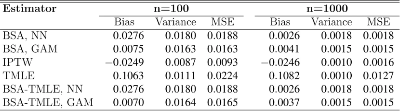
The first set of results in Table 1 demonstrate the balancing score prop-erty. The initial estimate Q¯0n is unadjusted. A correct logistic regression model is specified for g¯0, but predictions are transformed by the Beta
cumu-lative distribution function with both shape parameters equal to2. Although artificial, this means that g¯n converges to a monotone transformation of g¯0, which is a balancing score, but does not converge to the true g¯0. We can see
that the TMLE not adjusted for the propensity score and the IPTW estima-tors are not consistent as the bias is not decrease substantially when sample size increase. Conversely, methods where the initially estimateQ¯0nis adjusted with the propensity score, are consistent, as bias is decreasing quickly with sample size.
Table 2 shows similar performance in a more realistic scenario. In this setting, the initial estimator for Q¯0n is unadjusted, but the logistic regression model for the propensity score is misspecified by excluding the interaction termW1W2. Here predictions are not transformed. Hereg¯n is close to but not
exactly a balancing score, but it is close enough that the bias in estimators that nonparametrically adjust forg¯nis small. The IPTW estimator, however, is still biased at large n because g¯n is not converging to g¯0. In this case
TMLE performs well even with an unadjusted initial estimator but this is not guaranteed when g¯n is misspecified.
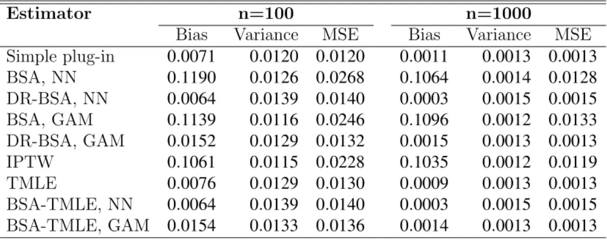
Table 3 examines the performance of estimators when the model for g¯0
is misspecified, (only including W1 in the logistic regression model,) but the initial estimate Q¯0n is a correctly specified model. Here we see that esti-mates that rely only on estimated propensity score, (the non-doubly robust BSA estimators and IPTW,) fail to be consistent, but estimates that use the
Table 1: Simulation results for distribution one with Q¯0n unadjusted and g¯n
correctly specified but transformed with Beta CDF
Estimator n=100 n=1000
Bias Variance MSE Bias Variance MSE BSA, NN 0.0276 0.0180 0.0188 0.0026 0.0018 0.0018 BSA, GAM 0.0075 0.0163 0.0163 0.0041 0.0015 0.0015 IPTW −0.0249 0.0087 0.0093 −0.0246 0.0010 0.0016 TMLE 0.1063 0.0111 0.0224 0.1082 0.0010 0.0127 BSA-TMLE, NN 0.0276 0.0180 0.0188 0.0026 0.0018 0.0018 BSA-TMLE, GAM 0.0070 0.0164 0.0165 0.0037 0.0015 0.0015
Table 2: Simulation results for distribution one with Q¯0n unadjusted, and g¯n
misspecified but close to a balancing score
Estimator n=100 n=1000
Bias Variance MSE Bias Variance MSE BSA, NN 0.0311 0.0166 0.0176 0.0027 0.0016 0.0016 BSA, GAM 0.0147 0.0159 0.0161 0.0033 0.0014 0.0014 IPTW 0.0390 0.0410 0.0425 0.0357 0.0025 0.0037 TMLE 0.0096 0.0172 0.0173 0.0098 0.0016 0.0017 BSA-TMLE, NN 0.0311 0.0166 0.0176 0.0027 0.0016 0.0016 BSA-TMLE, GAM 0.0101 0.0189 0.0190 −0.0042 0.0015 0.0016
Table 3: Simulation results for distribution one with Q¯0n correctly specified and g¯n misspecified
Estimator n=100 n=1000
Bias Variance MSE Bias Variance MSE Simple plug-in 0.0071 0.0120 0.0120 0.0011 0.0013 0.0013 BSA, NN 0.1190 0.0126 0.0268 0.1064 0.0014 0.0128 DR-BSA, NN 0.0064 0.0139 0.0140 0.0003 0.0015 0.0015 BSA, GAM 0.1139 0.0116 0.0246 0.1096 0.0012 0.0133 DR-BSA, GAM 0.0152 0.0129 0.0132 0.0015 0.0013 0.0013 IPTW 0.1061 0.0115 0.0228 0.1035 0.0012 0.0119 TMLE 0.0076 0.0129 0.0130 0.0009 0.0013 0.0013 BSA-TMLE, NN 0.0064 0.0139 0.0140 0.0003 0.0015 0.0015 BSA-TMLE, GAM 0.0154 0.0133 0.0136 0.0014 0.0013 0.0013
correctly specified initial estimate of Q¯0, are consistent. Importantly, even when the initial estimate is adjusted with the completely misspecified g¯n,
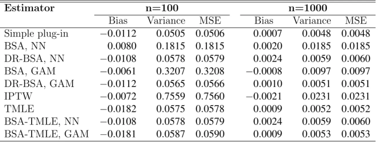
final estimates are still consistent when the initial Q¯0n is correctly specified. In a second scenario, called distribution two, Y is conditionally normal with α= (0,10,8,0,2) andβ = (−1,0,0,3,0). HereY depends onW1 andW2
but Adoes not, so they are not confounders. Additionally,Adepends onW3, but Y does not, so W3 is an instrumental variable. In this setting, because none of the baseline covariates are confounders, an unadjusted estimator of
ψ0will be consistent but not efficient, because it will fail to take into account
the relationship with the non-confounding baseline covariates W1 and W2. Here, the true ψ0 is 2 and the variance bound is approximately 5.1979/n.
Table 4 shows results from distribution two where the initial estimate for
¯
Q0 is the least squares estimate from a linear regression model with A, W1,
W2, andW3 are main terms, and the initial estimate for the propensity score
is the MLE from a logistic regression model with main terms W1, W2, and
W3. Here we see that, although all estimators have low bias, those that only adjust forg¯n, (the non-doubly robust BSA estimators and IPTW,) have much
higher variance than those with a correctly specified initial estimate. This demonstrates the importance in terms of efficiency of attempting to estimate
¯
Table 4: Simulation results from distribution two withQ¯0n correctly specified and g¯n correctly specified and includes an instrumental variable
Estimator n=100 n=1000
Bias Variance MSE Bias Variance MSE Simple plug-in −0.0112 0.0505 0.0506 0.0007 0.0048 0.0048 BSA, NN 0.0080 0.1815 0.1815 0.0020 0.0185 0.0185 DR-BSA, NN −0.0108 0.0578 0.0579 0.0024 0.0059 0.0060 BSA, GAM −0.0061 0.3207 0.3208 −0.0008 0.0097 0.0097 DR-BSA, GAM −0.0112 0.0565 0.0566 0.0010 0.0051 0.0051 IPTW −0.0072 0.7559 0.7560 −0.0021 0.0231 0.0231 TMLE −0.0182 0.0575 0.0578 0.0009 0.0052 0.0052 BSA-TMLE, NN −0.0108 0.0578 0.0579 0.0024 0.0059 0.0060 BSA-TMLE, GAM −0.0181 0.0587 0.0590 0.0009 0.0053 0.0053
6
Discussion
In this paper we discuss the balancing score property of estimators that nonparametrically adjust for the propensity score. We see in simulations that even when the propensity score estimator is not consistent,Ψ(P0)can be
estimated with low bias if the estimate of the propensity score approximates a balancing score well enough. Additionally we introduce a balancing score adjusted TMLE which has the balancing score property and is also doubly robust and locally efficient, and provide regularity conditions for asymptotic linearity in Appendix A.
The estimators present in this paper are for the statistical parameter
E0[E0(Y |A=1,W)], which, under assumptions, can be interpreted as the population mean of a variableY whenY is subject to missingness (Kang and Schafer, 2007). The results and similar estimators are immediately applicable to other interesting statistical parameters such as
E0[E0(Y |A=1,W)−E0(Y |A=0,W)]
and
which, under non-testable causal assumptions, can be interpreted as causal parameters called the ATE or ATT, respectively (Hahn, 1998, van der Laan and Rose, 2011). Additionally, the results are immediately generalizable to the estimation of parameters in marginal structural models (Robins, 1997, Rosenblum and van der Laan, 2010).
Traditionally, propensity score based estimators estimate the propensity score based on how well g¯n approximates the trueg¯0. Collaborative targeted
minimum loss-based estimation (CTMLE) is a method that chooses an es-timator for the propensity score based on how well it helps reduce bias in the estimation of Ψ(P0) in collaboration with an initial estimate of Q¯0 using
cross-validation (van der Laan and Gruber, 2010, van der Laan and Rose, 2011). In doing so, CTMLE attempts to adjust the propensity score for the most important confounders first, and avoid adjustment for instrumen-tal variables. This can lead to improvements in efficiency and robustness to violations of the assumption P0(A=a|W)>0. Applying an analogous tech-niques of estimator selection for balancing score adjusted estimators is an area of further research.
References
A. Abadie and G.W. Imbens. Bias-corrected matching estimators for average treatment effects. Journal of Business & Economic Statistics, 29(1):1–11, 2011.
Peter C Austin. The performance of different propensity-score methods for estimating differences in proportions (risk differences or absolute risk re-ductions) in observational studies. Statistics in medicine, 29(20):2137–48, September 2010. ISSN 1097-0258. doi: 10.1002/sim.3854.
Peter J. Bickel, Chris A. J. Klaassen, Ya’acov Ritov, and Jon A. Wellner.
Efficient and Adaptive Estimation for Semiparametric Models. The Johns Hopkins University Press, Baltimore, 1993. ISBN 0801845416.
M. Caliendo and S. Kopeinig. Some practical guidance for the implemen-tation of propensity score matching. Journal of economic surveys, 22(1): 31–72, 2008.
non-experimental causal studies. Review of Economics and statistics, 84(1): 151–161, 2002.
S. Gruber and M.J. Van Der Laan. A targeted maximum likelihood estimator of a causal effect on a bounded continuous outcome. The International Journal of Biostatistics, 6(1), 2010.
Jinyong Hahn. On the role of the propensity score in efficient semiparamet-ric estimation of average treatment effects. Econometrica, 66(2):315–331, March 1998. ISSN 0012-9682. doi: 10.2307/2998560.
J.D.Y. Kang and J.L. Schafer. Demystifying double robustness: a comparison of alternative strategies for estimating a population mean from incomplete data. Statistical science, 22(4):523–539, 2007.
J.K. Lunceford and M. Davidian. Stratification and weighting via the propen-sity score in estimation of causal treatment effects: a comparative study.
Statistics in medicine, 23(19):2937–2960, 2004.
P. McCullagh and J.A. Nelder. Generalized linear models, volume 37. Chap-man & Hall/CRC, 1989.
R Core Team. R: A Language and Environment for Statistical Computing. R Foundation for Statistical Computing, Vienna, Austria, 2012. URL
http://www.R-project.org/. ISBN 3-900051-07-0.
James M. Robins. Marginal structural models. InProceedings of the Ameri-can Statistical Association. Section on Bayesian Statistical Science, pages 1–10, 1997.
J.M. Robins, M. ´A. Hern´an, and B. Brumback. Marginal structural models and causal inference in epidemiology. Epidemiology, 11(5):550–560, 2000. P.R. Rosenbaum. Model-based direct adjustment. Journal of the American
Statistical Association, 82(398):387–394, 1987.
P.R. Rosenbaum and D.B. Rubin. The central role of the propensity score in observational studies for causal effects. Biometrika, 70(1):41, April 1983. P.R. Rosenbaum and D.B. Rubin. Reducing bias in observational studies
using subclassification on the propensity score. Journal of the American Statistical Association, 79(387):516–524, 1984.
Michael Rosenblum and Mark J van der Laan. Targeted maximum likeli-hood estimation of the parameter of a marginal structural model. The international journal of biostatistics, 6(2):Article 19, January 2010. ISSN 1557-4679. doi: 10.2202/1557-4679.1238.
Jasjeet S. Sekhon. Multivariate and propensity score matching soft-ware with automated balance optimization: The Matching package for R. Journal of Statistical Software, 42(7):1–52, 2011. URL
http://www.jstatsoft.org/v42/i07/.
Mark J. van der Laan. Targeted Maximum Likelihood Based Causal Infer-ence: Part I. The International Journal of Biostatistics, 6(2), January 2010a. ISSN 1557-4679. doi: 10.2202/1557-4679.1211.
Mark J van der Laan. Targeted maximum likelihood based causal inference: Part II. The international journal of biostatistics, 6(2), January 2010b. ISSN 1557-4679. doi: 10.2202/1557-4679.1241.
Mark J van der Laan and Susan Gruber. Collaborative double robust targeted maximum likelihood estimation. The international journal of biostatistics, 6(1), January 2010. ISSN 1557-4679. doi: 10.2202/1557-4679.1181.
Mark J. van der Laan and Sherri Rose. Targeted Learning: Causal Inference for Observational and Experimental Data. Springer, New York, 2011. ISBN 1441997814.
Mark J. van der Laan and Daniel Rubin. Targeted Maximum Likelihood Learning. The International Journal of Biostatistics, 2(1), January 2006. ISSN 1557-4679. doi: 10.2202/1557-4679.1043.
Mark J van der Laan, Eric C Polley, and Alan E Hubbard. Super learner.
Statistical applications in genetics and molecular biology, 6(1), January 2007. ISSN 1544-6115. doi: 10.2202/1544-6115.1309.
A. W. van der Vaart. Asymptotic statistics. Cambridge University Press, Cambridge, UK New York, NY, USA, 1998.
A. W. van der Vaart and Wellner J. A. Weak convergence and empirical processes. Springer, New York, 1996.
Simon N. Wood. Fast stable restricted maximum likelihood and marginal likelihood estimation of semiparametric generalized linear models. Journal of the Royal Statistical Society: Series B (Statistical Methodology), 73(1): 3–36, 2011. ISSN 1467-9868. doi: 10.1111/j.1467-9868.2010.00749.x. Wenjing Zheng and Mark J Van Der Laan. Asymptotic Theory for
Cross-validated Targeted Maximum Likelihood Estimation. Working Paper 273, U.C. Berkeley Division of Biostatistics Working Paper Series, 2010. URL
http://www.bepress.com/ucbbiostat/paper273/.
Wenjing Zheng and Mark J van der Laan. Targeted maximum likelihood esti-mation of natural direct effects. The international journal of biostatistics, 8(1), January 2012.
A
Some results and proofs
Proof of Lemma 1. In this proof, E means expectation with respect to P. First note thatE(Y |A=1,W,b(W)) =E(Y |A=1,W)becausebis a function of onlyW. Next,
E[E(Y |A=1,W)|A=1,b(W)] =E[E(Y |A=1,W)|b(W)]
because the inner conditional expectation is a function of only W and W ⊥ A|b(W) when b is a balancing score. Thus,
E[E(Y |A=1,b(W))] =E{E[E(Y |A=1,W,b(W))|A=1,b(W)]}
=E{E[E(Y |A=1,W)|A=1,b(W)]}
=E{E[E(Y |A=1,W)|b(W)]}
=E[E(|A=1,W)] =Ψ(P)
Lemma 2. Ifg¯ntakes only discrete values with supportG, thenΨ((Q¯0n,QW n))
is a TMLE if θ0 is estimated in a saturated parametric model
logitQ¯0n(θ)(a,w) =logit(Q¯0n(A,W)) +
∑
a∈{0,1}c∈G
where Q¯0n is some initial estimator for Q¯0, Q¯0n=Q¯0n(θn) andI is the indicator
function.
Proof of Lemma 2. The MLEθn(or empirical risk minimizer for the negative
quasi-binomial log likelihood, ifY is not binary), solves the score equations for each parameter θa,c:
0=
n
∑
i=1
I(Ai=a,gn(1|Wi) =c)(Y−Q¯0n(Ai,Wi))
whereQ¯0n(a,w) =Q¯0n(θn)(a,w). Additionally, any functionhofAandgn(1|W)
is in the linear span of basis functionsI(A=a,gn(1|W) =c)for all a∈ {0,1},
c∈G, so 0= n
∑
i=1 h(Ai,gn(1|Wi))(Y−Q¯1n(Ai,Wi)).In particular, the above equation is solved when h(a,w) = g a
n(1|w), which is
the score from the parametric submodel in (5). Thus if the TMLE update is applied to the estimate Q¯0n, εn =0, and Q¯∗n =Q¯0n so Ψ((Q¯0n,QW n)) is a
TMLE.
Lemma 3. The function b is a balancing score if and only if there exists some function φ such that φ(b(w)) =g0(w) a.e..
Proof. Suppose b is a balancing score. By definition of the propensity score and the property of the balancing score, we know that
g0(W) =E0(A|W) =E0(A|W,b(W)) =E0(A|b(W)).
Thus g¯0(W) =φ(b(W)), whereφ(x) =E0(A|b(W) =x), which proves that if
bis a balancing score, then there exists some functionφ such thatφ(b(w)) = g0(w)a.e..
Suppose now that g¯0(w) =φ(b(w)) a.e. for some φ. We have E0(A|
b(W),W) =g0(W), but sinceg¯0(W) =φ(b(W)), it follows thatE0(A|b(W),W) =
φ(b(W)) and thus that E0(A|b(W),W) =E0(A|b(W)) so b is a balancing
Theorem 3. Define Φ1(Q) =P0Q¯g¯−g¯g¯0 and Φ2(g) =P0(Q¯−Q¯0)g0¯g¯. Assume
D∗(Q∗n,gn)falls in aP0-Donsker class with probability tending to 1;P0{D∗(Q∗n,gn)− D∗(Q,g)}2→0 in probability as n→∞; P0(Q¯0−Q¯∗ n)(g¯0−g¯n) (g¯−g¯n) ¯ gg¯n = oP(1/ √ n); P0(Q¯∗n−Q¯)(g¯n−g¯)/g¯ = oP(1/√n); P0(Q¯−Q¯0)(g¯−g¯0)/g¯ = 0;
Φ1(Q¯∗n) andΦ2(g¯n) are asymptotically linear estimators ofΦ1(Q¯) and Φ2(g¯)
with influence curves IC1 and IC2, respectively.
ThenΨ(Q∗n)is asymptotically linear with influence curveD∗(Q,g) +IC1+
IC2.
Proof. Since P0D∗(Q,g) =ψ0−Ψ(Q) +P0(Q¯0−Q¯)(g¯0−g¯)/g¯ (e.g, Zheng and
Laan (2010), Zheng and van der Laan (2012)), where we use the notation
¯
g(W) =g(1|W) and Q¯(W) =Q¯(1,W), this results in the identity:
Ψ(Q∗n)−ψ0= (Pn−P0)D∗(Q∗n,gn) +P0(Q¯0−Q¯∗n)(g¯0−g¯n)/g¯n.
The first term equals (Pn−P0)D∗(Q,g) +oP(1/√n)if D∗(Qn∗,gn) falls in aP0 -Donsker class with probability tending to 1, andP0{D∗(Q∗n,gn)−D∗(Q,g)}2→
0 in probability asn→∞(van der Vaart and A., 1996, van der Vaart, 1998).
We write
P0(Q¯0−Q¯∗n)(g¯0−g¯n)/g¯n=P0(Q¯0−Q¯∗n)(g¯0−g¯n)/g¯+P0(Q¯0−Q¯∗n)(g¯0−g¯n)(g¯−g¯n)
¯ gg¯n
.
Assume that the last term is oP(1/√n). We now write
P0(Q¯0−Q¯∗n)(g¯0−g¯n)/g¯=P0(Q¯∗n−Q¯+Q¯−Q¯0)(g¯n−g¯+g¯−g¯0)/g¯
=P0(Q¯∗n−Q¯)(g¯n−g¯)/g¯+P0(Q¯∗n−Q¯)(g¯−g¯0)/g¯
+P0(Q¯−Q¯0)(g¯n−g¯)/g¯+P0(Q¯−Q¯0)(g¯−g¯0)/g¯ ≡P0(Q¯∗n−Q¯)(g¯n−g¯)/g¯+Φ1(Q¯n∗)−Φ1(Q¯)
+Φ2(g¯n)−Φ2(g¯) +P0(Q¯−Q¯0)(g¯−g¯0)/g¯,
whereΦ1(Q) =P0Q¯g¯−g¯g¯0 and Φ2(g) =P0(Q¯−Q¯0)g0g¯¯. We assume that the first
term is oP(1/√n), the last term equals zero (i.e., either g=g0 or Q¯ =Q¯0), and Φ1(Q¯∗n) and Φ2(g¯n) are asymptotically linear estimators with influence
curves IC1 and IC2, respectively. This proves Ψ(Q∗n) is asymptotically linear
B
TMLE when
Y
is not bounded by
0
and
1
If Y is not bounded by 0 and 1, but we can assume Y is bounded by l and
u with −∞<l<u<∞,Y can be transformed toY†=Yu−−ll. Similarly Q¯0n can
be transformed to Q¯0†n = Q¯0n−l
u−l . The procedure described in Section 3 can be
applied to the data structure(W,A,Y†)usingQ¯0†n as initial estimator, and the final estimate can be transformed back to the original scale asΨ((Q¯∗n,QW n))∗
(u−l) +l. When l and u are not known, they can be set to the minimum and maximum of the observedY as described in (Gruber and Van Der Laan, 2010).
For completeness we can define an alternative TMLE using a linear work-ing model where
¯
Qn0(ε)(A,W) =Q¯0n(A,W) +ε A gn(1|W)
with loss function
LY(Q¯)(O) = (Y−Q¯(A,W))2
the squared error loss. Here, ε0=arg minεE0LY(Q¯)(O) can be estimated by
standard least squares regression software, with Q¯0n(A,W) as an offset. Asymptotically, a TMLE using a linear working (or linear fluctuation) is the equivalent to a TMLE with a logistic working model, but in practice can perform poorly. This is because if gn(1|Wi) is very small for some observa-tions, which is more likely in small samples,εn0can be large in absolute value,
having a large effect on Q¯∗n with a linear fluctuation, which is unbounded. Because of this, if it is reasonable to boundY by some l andu, it the logistic working model is recommended because Q¯∗n always respects these bounds, even if εn0 is large.