Conflict Resolution in Mobile Networks: A
Self-Coordination Framework Based on
Non-dominated Solutions and Machine
Learning for Data Analytics
Jessica Moysen, Department of Signal and Theory Communications, Universitat
Polit`ecnica de Catalunya-UPC, Barcelona, Spain
Mario Garc´ıa-Lozano, Department of Signal and Theory Communications,
Universitat Polit`ecnica de Catalunya-UPC, Barcelona, Spain
Lorenza Giupponi, Communications and Network Division, Centre Tecnol`ogic de
Telecomunicacions de Catalunya-CTTC, Barcelona, Spain
Silvia Ru´ız, Department of Signal and Theory Communications, Universitat
Polit`ecnica de Catalunya-UPC, Barcelona, Spain
Abstract
Self-organizing network (SON) is a well-known term used to describe an autonomous cellular network. SON functionalities aim at improving network operational tasks through the capability to configure, optimize and heal itself. However, as the deployment of independent SON functions increases, the number of dependencies between them also grows. This work proposes a tool for efficient conflict res-olution based on network performance predictions. Unlike other state-of-the-art sres-olutions, the proposed self-coordination framework guarantees the right selection of network operation even if conflicting SON functions are running in parallel. This self-coordination is based on the history of network measurements,
which helps to optimize conflicting objectives with low computational complexity. To do this, machine learning (ML) is used to build a predictive model, and then we solve the SON conflict by optimizing more than one objective function simultaneously. Without loss of generality, we present an analysis of how the proposed scheme provides a solution to deal with the potential conflicts between two of the most important SON functions in the context of mobility, namely mobility load balancing (MLB) and mobility robustness optimization (MRO), which require the updating of the same set of handover parameters. The proposed scheme allows fast performance evaluations when the optimization is running. This is done by shifting the complexity to the creation of a prediction model that uses historical data and that allows to anticipate the network performance. The simulation results demonstrate the ability of the proposed scheme to find a compromise among conflicting actions, and show it is possible to improve the overall system throughput.
I. INTRODUCTION
A cellular network with intelligence and autonomous capabilities is called a self-organizing network (SON). The SON was introduced by the 3rd Generation Partnership Project (3GPP) as a key component of Long Term Evolution (LTE) networks, starting from the first release of this technology (Release 8) and expanding in the subsequent ones. The 3GPP has defined the main areas of the SON in [1], which are classified into configuration, healing and self-optimization. In addition, the 3GPP defined the minimization of drive tests (MDT) functionality in Release 9. This feature enables operators to collect user equipment (UE) measurements, with the purpose of optimizing network management [2]. Finally, in order to handle the potential conflicts that may exist due to the parallel execution of multiple SON functions, the self-coordination concept was introduced in Release 10 [3].
In this paper, we discuss the self-coordination problem. In particular, we focus on the output parameter SON conflict, i.e., when two or more SON functions aim at adjusting the same output parameter with opposite values. So, a SON coordinator controlling the actions of the SON functions during operation is considered a necessity [4]. In order to evaluate the performance of the proposed scheme, we focus on the handover management issue. We consider a well-known
SON conflict between mobility load balancing (MLB) and mobility robustness optimization (MRO). MLB and MRO are two of the most important self-optimization functions that deal with mobility management. Both mechanisms modify the behavior of handover, which is a procedure that allows connections to be transferred between base stations in a seamless manner. However, each one pursues a different objective:
• MLB aims at balancing traffic load among cells so that cells with excess traffic (congested cells) can transfer some of their users to less loaded neighboring cells and vice versa. This can be done by changing the parameters that govern UE cell selection, such as handover thresholds, hysteresis margins and times to trigger a handover event. The primary goal is to achieve a higher system capacity, and this is done by distributing UE traffic across the available radio resources in the system.
• On the other hand, MRO is designed to improve mobility robustness:
– Minimization of call drops due to radio link failures: Depending on how the handover parameters are adjusted, too-early handovers may happen for some users. This means that the communication fails due to high propagation losses with the new cell. Similarly, too-late handovers may imply that communication with the serving base station is lost before a new connection is established.
– Minimization of unnecessary handovers: Too-short time-of-stays in the new cell or ping-pong (quick handover back to the previous cell) should not happen. For example, a vehicular user moving in a city where macrocells coexist with a layer of small cells should utilize a larger timer to trigger handovers toward picocells. This should avoid handovers from macro- to picocells, where vehicular users with high speed would have very short time-of-stays. Note that this would cause data throughput degradation due to the high volume of signaling transmission required to repeatedly update the serving cell.
with independent objectives. However, if both are applied in parallel and without coordination, the actions requested by each SON function may be different. They may cause opposite changes in handover parameters, and so, they may enter into a conflict. Under these circumstances, the system would enter into a cycle of constant re-configuration, thereby causing performance degradation due to excessive signaling that requires radio resources.
In this context, machine learning (ML) is proposed as a candidate tool that allows the network to learn from experience and solve conflicts in an effective manner. The main feature is that the network is able to run different SON functions in parallel and improve the system performance. In particular, thanks to the use of a variety of techniques from data mining, statistics and ML, it is possible to analyze historical data to make predictions about unknown future events. This is known as predictive analytics and for the current work, it turns the network management from reactive to predictive. In this context, big data analytics are currently receiving big attention due to their capability to provide insightful information from the analysis of high volumes of data that are readily available for operators.
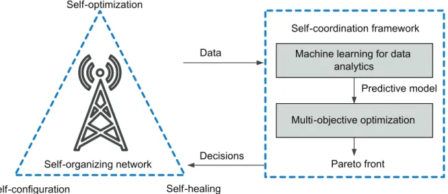
Based on that, the motivation behind this paper is to provide a tool that allows mobile network operators to become proactive by anticipating behaviors and making decisions accordingly. We focus on building a tool for efficient self-coordination that is based on the network performance prediction that is made by doing a proper data analysis of UE measurements. The tool works in two steps as graphically depicted in Figure 1:
1) In the first step, the proposed scheme learns from past experience to obtain a network performance predictor for each SON function individually. In particular, ML is used for data analytics. Available measurements are globally utilized in a learning process that yields an estimator by means of regression models.
2) Then, performance predictions are the inputs of a multi-objective optimization process, which searches for a set of non-dominated solutions or Pareto front. That is to say, the solutions cannot improve the performance of one SON function without degrading the
Self-organizing network Self-configuration Self-optimization Self-healing Data Predictive model Self-coordination framework Decisions Pareto front Machine learning for data
analytics
Multi-objective optimization
Fig. 1: Self-coordination framework.
other one. In this paper, we select the Non-dominated Sorting in Genetic Algorithms II (NSGA-II), which is able to obtain a better spread of solutions with lower computational complexity than other algorithms [5].
In summary, the self-coordination framework aims at guaranteeing the operator’s needs by finding the operating point that provides the best performance trade-off when an SON conflict happens. This is done through the multi-objective optimization process, which uses the insights from big data (i.e., it uses the patterns found in historical data) to predict the performance metric of each SON function, and then it searches for a representative subset of solutions that are non-dominated to each other.
This paper is organized as follows. Section II describes previous works and relates them to the current research. In Section III, we describe the self-coordination framework, its main design principles and the algorithms that we use to build it. In the same section, we discuss design details, the fine-tuning of the prediction model (Section III-A), and the multi-objective optimization process (Section III-B). In Section IV, we present the details of our particular case of study (MLB-MRO SON conflict) where the proposed scheme is applied. Section V
describes the simulation platform and test scenarios. Subsequently, the simulation results and the corresponding discussion are presented. Finally, Section VI concludes this paper.
II. RELATEDWORK AND CONTRIBUTIONS
As we stated earlier, in order to guarantee a correct network operation, the SON functions have to be coordinated. Examples of solutions for the self-coordination problem can be found in [6], [7]. In [6], the authors focus on a preventive coordination mechanism that uses a policy-based decision process. The proposed scheme contains a policy engine to make automated operational decisions but under the control of the operator. That is to say, operators can decide which SON functions to execute by changing the rules that determine system behavior in a particular situation. However, in this solution, they address the coordination of a single SON function among the different cells. In [7], the authors propose a solution for the concurrent execution of multiple SON functions. They demonstrate that the proposed approach is able to coordinate several SON functions by taking advantage of game theory. To do that, each SON function is modeled as a Markov decision process (MDP) and solved by means of reinforcement learning (RL). However, a scalability vs. convergence trade-off arises and a detailed analysis is needed due to the required computational cost. Indeed, our approach tackles the conflict resolution problem for multiple SON functions addressing real-time computational requirements. In particular, it shifts processing complexity to the creation of a predictive model to be used when the network is in exploitation. This allows it to make fast and still accurate evaluations of the actions that are being evaluated by the SON coordinator and, hence, to make appropriate decisions in real time.
Since the implementation of MLB has a negative impact on the performance of MRO, the interaction between these two SON functions has received increased interest among researchers in this field. The work in [8] focuses on solving this conflict by adjusting the handover parameters taking into account the traffic load distribution. MLB modifies the handover parameters of the serving and the neighboring cells considering the MRO performance metrics and the load level
of the neighboring cells. This way, it ensures a reduction in the number of early and too-late handovers and radio link failures while balancing the load among cells. This solution does not take advantage of learning from past experience, and decisions are always made based on instantaneous network information. Therefore, there is room to further minimize erroneous decisions. In this context, an example of an RL application for MLB-MRO SON conflict can be found in [9] and [10]. In both works, the authors take advantage of experience gained from past decisions in order to reduce uncertainty about the impact of the actions taken to resolve conflicts. The authors in [9] propose the use of Q-learning as an RL method. However, value-based methods such as Q-learning may compromise feasibility since they require a huge state (and action) space. Different authors provide a wide variety of strategies to reduce complexity such as function approximation and state space aggregation. The authors in [10] follow the latter while employing general policy iteration (GPI) [11]. The authors demonstrate that by using this method, the operator’s needs can be met. However, the drawback of policy-based methods is that they suffer from high variance in the quality of results and they only consider a small subset of solutions so there is a certain probability that good solutions are not evaluated.
We propose to solve the self-coordination problem by means of multi-objective evolution-ary algorithms in combination with ML. The use of multi-objective optimization alone would be unfeasible since the search for the solutions requires multiple performance evaluations to be done by means of system-level simulations. A real-time execution of this process would be absolutely unfeasible and this is one of the biggest problems in existing multi-objective approaches. Thanks to the use of ML, we can capitalize on the big data available in mobile networks and create a prediction model that allows real-time multi-objective optimizations. The proposed scheme exploits both components working together, namely, big data analytics and multi-objective optimization. In this regard, we found several works in the literature regarding the benefits of big data in 5G networks, such as [12], [13], where the authors identify different sources of data that can act as an input to the SON entity, e.g., to perform load balancing and
prediction operations, among others.
In this work, we take advantage of the MDT functionality (enhanced in Release 11) by collect-ing measurements indicatcollect-ing throughput and connectivity issues to estimate network performance. The exploitation of these huge amounts of data is analyzed with regression analysis, where the primary goal is to predict UE performance. We consider the analysis of our previous works [14]–[16], where the exploitation of the huge amount of data is analyzed with regression models to make better decisions for management purposes. In particular, our work in [15] focuses on two families of regression models, linear and nonlinear. A comparison was performed among different models, selected on a basis of low complexity and high accuracy. Prediction results were analyzed for different kinds and amounts of UE measurements. Based on the outcomes of that research, in this new work, we focus on bagging in combination with the support vector machine (SVM), referred to hereafter as the Bagged-SVM method.
Since we aim to find a trade-off between different goals, once the predictive model has been built, we solve the SON conflict by means of multi-objective optimization, and in particular, multi-objective evolutionary algorithms that use non-dominated sorting [5]. These kinds of algorithms are based on meta-heuristics that simulate the process of natural evolution and operate efficiently when a large number of parameters need to be configured simultaneously. While the multi-objective problem formulation presented herein can be solved by means of RL [17], it is important to note that following this approach, the agent needs a good strategy to explore the environment within a reasonable amount of time. Therefore, in this paper we have supplied the agent with NSGA-II, which is able to maintain a spread of solutions with a lower computational complexity.
Given this, the contributions of this paper can be summarized as follows:
X We present a tool for an efficient SON conflict resolution based on network performance predictions. A prediction model is created by extracting relevant information from the mobile network. This allows the operator to anticipate system behavior to make effective decisions in real-time. Scalability is guaranteed since the processing complexity is shifted
Itf-N Self-coordination framework Response i c2 i c1 2 SON 1 Cell Action requests M Cell 1 SON N SON i Cell 2 SON 1 SON N SON 2 SON 1 SON N SON 1 1 c 1 2 c 1 N
c
c
iNc
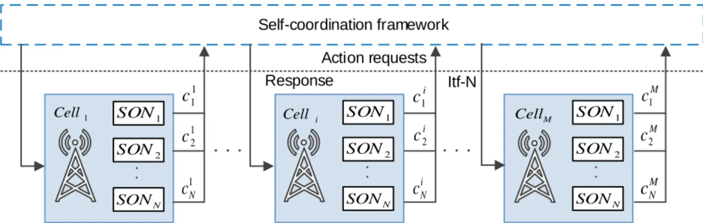
NM M c2 M c1Fig. 2: Each SON function requests the adjustment of different network parameters of cell i, and each one sends the action requests to the self-coordination framework.
to the creation stage of the model, allowing fast performance evaluation when optimization is running.
X In order to evaluate the proposed scheme, we analyze, without loss of generality, the MLB-MRO SON conflict. The simulation results show that the proposed scheme can not only solve the SON conflict but also improve overall system throughput.
III. GENERALSELF-COORDINATION FRAMEWORK
We consider a wireless network composed of a set M = {1, . . . , M} of M=|M| cells regularly deployed with inter-site distanceD. On each cell j = (1, . . . , N), we consider N SON functions running in parallel. We denote by c(j) = (c(j)
1 , . . . , c (j)
N ) the configuration parameter
vector of a cell j, with c(ij) denoting the value for the parameter of the SON function i, e.g., the transmission power (TXP), the antenna tilt (TILT), the action to switch ON or OFF the cell, handover parameters such as the Cell Individual Offset (CIO), hysteresis margin (HYS) or time to trigger (TTT). The N SON functions are implemented on every cell, which must send a request to the SON coordinator and get a positive response in order to adjust some of its parameters. These requests and responses are represented in Figure 2 with the links between each cell and the SON coordinator and they must pass through the interface-N (Itf-N). We propose to solve
the challenge of coordination among SON functions by analyzing their interactions based on the measurement history of the network. To do this, we design the self-coordination framework based on two main functions: 1) machine learning for data analytics, and 2) multi-objective optimization. Each is depicted in Figures 3 and 4, respectively, and described in the subsequent subsections.
A. Machine learning for data analytics
The main objective of this function is to analyze large amounts of data sets to uncover hidden patterns, correlations and other useful information to make better decisions. This is done by considering the UE measurement reports, which contain power and quality measurements from the serving and neighbor base stations:
- Reference Signal Received Power (RSRP): Average power received from LTE reference signals, used for channel estimation and handover/cell selection.
- Reference Signal Received Quality (RSRQ): Ratio between the total power received from reference signals and the total power received in the full bandwidth. The RSRQ mea-surement provides additional information about interference levels to make a reliable han-dover/cell reselection decision.
Once the data have been collected, we perform a data preparation process to extract and analyze the radio measurements. To do that, we propose to make use of ML techniques, which have been demonstrated to be very effective for making predictions based on observations. Among the most important ML tools for data analysis, we focus on regression analysis. It is important to note that evaluating the network performance for a given configuration requires a dynamic system-level simulation, which requires high computational time. If several configurations need to be assessed during the optimization, the computational cost is indeed prohibitive. So, regression analysis shifts the processing complexity to the model creation stage and allows fast performance evaluations when optimization is running.
Partitioning data Processing data Collecting data Training data Testing data Model Model validation Bagged-SVM
Fig. 3: Machine learning for data analytics.
Collect n measurements (new data)
s
s
1,..., psize Prediction function Model Metric predicted Genetic operations Reach stopping criteria Pareto front no yesFig. 4: Multi-objective optimization.
Regression analysis is an ML technique, which allows us to predict the performance metric of each SON function. Regression takes an input vector (x) and an output value (y) to develop a predictive model, returning the predicted output yˆ. We represent the input space by an n -dimensional input vectorx= (x(1), . . . , x(n))T ∈Rn, where each dimension is an input variable.
The size of the input space is [x×n]. The number of rows is the number of UEs at any place and anywhere, and the number of columns corresponds to the number of measurements n. In addition, a set involves m samples ((x1, y1), . . . ,(xm, ym)). Each sample consists of an input
vectorxi, and a corresponding output yi, which represents the UE performance indicator. Hence
x(ij) is the value of the input variable x(j) in sample i, and the error is usually computed via
|yˆi−yi|. To evaluate the accuracy of the model, after the data have been collected and normalized,
we randomly select 3/4 of the data to be the training set (x.train, y.train), and place the rest into the testing set (x.test, y.test).
A well-known paradigm to improve the accuracy of regression models is ensemble learning, which combines multiple weak learners to solve the same problem. This approach usually produces more accurate solutions than a single model would. In this sense, one of the most useful techniques is bagging [18]. Bagging improves regression by subsampling the training samples and randomly generating training subsets. Then, it runs the learning algorithms several times, each one with a different subset, and a final regressor is obtained by averaging the different outputs. As we stated earlier, in this work, we focus on bagging in combination with SVM, referred to hereafter as the Bagged-SVM method.
SVM analysis is a popular ML tool for classification and regression, first identified byVladimir Vapnikin [19]. The motivation to use SVM is that this method shows high accuracy in predictions and we can obtain good behaviors with nonlinear problems. For the current problem, given ((x1, y1), . . . ,(xm, ym)), the goal is to find a function f(x) that deviates from yn by a value no
greater than . The main idea is to characterize the optimal hyperplane, which will approximate all training samples with the required precision. For this purpose, the problem can be mapped onto a higher dimensional space. This allows the points to be relocated onto another space such that they become linearly separable and the fit is easier. In particular, data are transformed into a higher dimensional space by means of kernel functions. Since nonlinear kernels can be used, nonlinear regression is also possible. The estimation accuracy depends on the setting of the
precision, the kernel parameters and the regularization parameter c[20]. Hence, we tune these parameters to generate predictions by creating a model on a subset of training samples. For further details on the theory behind SVM, the reader is referred to [21], [22].
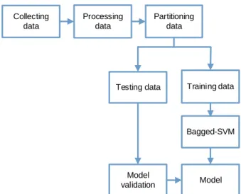
The whole process is depicted in Figure 3 and summarized as follows:
1) Collecting data. For each UE, we collect RSRP and RSRQ from the serving and neighbor-ing cells. To test the performance of each SON function, different metrics are obtained. 2) Processing data. Once data are collected, they are prepared by normalizing every variable. 3) Partitioning data. To validate the model to be created, observations are partitioned into two
sets, one for calibration and the other for validation.
4) Building the ML models. We select the SVM regression model, where in order to enhance the performance of the learning algorithm, multiple data sets are used by means of the bagging technique. SVM is then applied to produce a regressor. For each test value, we predict and evaluate its performance against the actual value in terms of root mean square error (RMSE).
The model produced by the regressive algorithm is the input to the multi-objective optimization process described below.
B. Multi-objective optimization
As we stated earlier, we consider the situation in which optimizing a particular solution with respect to a single SON objective can result in unacceptable results with respect to the other SON objectives. That is, the parallel execution of N SON functions may generate a resource conflict if at least two of them request to adjust parameters in a way that cancels the actions the other one intends to take. Therefore, potential conflicts may occur, that will cause degradation of network performance. In this context, multi-objective optimization is a promising tool to find the point that provides the best trade-off performance of conflicting SON functionalities. In particular, we use multi-objective evolutionary algorithms to find a compromise between multiple SON functions. Evolutionary algorithms are population-based meta-heuristic algorithms
that are capable of obtaining a set of solutions simultaneously, so they are very suitable to solve multi-objective optimization problems. The general approach determines an entire Pareto optimal solution set or Pareto front. This is a representative subset of solutions that are non-dominated with respect to each other. These kinds of solutions cannot improve any of the objectives without conflicting with at least one of the other objectives, i.e., optimizing a decision vector (s) with respect to a single objective often degrades other objectives. As a consequence, a reasonable solution to a multi-objective problem is to find a set of solutions that satisfies the objectives at an acceptable level without being dominated by any other solution. That is, the final solution of the decision-maker is always a trade-off.
s1 s2 .. . sn → SON1 SON2 .. . SONN → F1 F2 .. . FK
Let us consider N SON functions that pursue the optimization of K objectives. A minimization problem with K objectives can be formulated as follows:
minimize (F1(s), F2(s), . . . , FK(s))
subject to s∈S
where s = s1, . . . , sn is an n-dimensional decision variable vector in the solution space S.
Thus, the objective is to find an objective vectors∗ (feasible solution) that minimizes a given set of K objective functions, i.e., we say that s∗ is Pareto optimal if there is no alternative vector s where improvements can be made to at least one SON objective function without reducing another one.
Among the multi-objective formulations available in the literature, we use NSGA-II [5]. The reason for using this approach is that these kinds of methods take advantage of genetic algorithms (GAs), which are heuristic algorithms that can adapt their objective functions to the
multi-objective problem. GAs are able to improve partial solutions since they create new individuals by performing selection, crossover and mutation, but at the same time they keep the best individuals (i.e., the elitism). In this regard, NSGA-II allows less computational complexity than other evolutionary algorithms, and it also prevents the loss of good solutions once they are found since it preserves the elitism.
The concept of GA was introduced by Holland in [23]. GAs are inspired by the evolutionary theory explaining the natural selection. In GAs, a solution vector is called a chromosome, which is represented by a series of genes made of discrete units. Each unit controls one or more of the chromosome features. A chromosome corresponds to a unique solution s in the solution space S. GAs manage a set of chromosomes or population, which is usually initialized by random valid solutions. As the search evolves, the population eventually converges to a single solution. To do that, the two most important operators are crossover and mutation. Crossover combines two parent chromosomes to form two new solutions called offspring. By iteratively applying the crossover operator, the best offsprings appear more frequently in the population, leading to convergence toward a good solution. On the other hand, mutation introduces genetic diversity in the population by means of random alterations in the offspring. The probability of mutation is very small and depends on the length of the chromosome. Therefore, the new chromosome produced by mutation will not be very different from the original one.
Given this, the procedure is adapted to our particular problem as follows: NSGA-II starts with a random initial population s1, . . . ,spsize of size p
size. Each feasible solution corresponds to a
vector of size M, where each value denotes the network parameter to be optimized, which is associated with each cell. In order to evaluate the fitness of each chromosome, in each iteration
t, we collect n0 measurements at some arbitrary points in the scenario. These measurements are obtained as a consequence of having configured the parameters of the scenario according to each chromosome s. These n0 measurements (new data) and the built model already described in Section III-A, are the inputs to the prediction function, which gives us the UE performance.
As a result, for each s ∈ S, we obtain a predicted performance metric. The algorithm applies crossover and mutation to create an offspring population. In generationt, an offspring population of sizepsize is created from the parent population, and non-dominated fronts F1, F2, . . . , FK are
identified in the combined population. The next population is filled starting from solutions in
F1, then F2, and so on. A high-level overview of the process is depicted in Figure 4.
In summary, we first exploit the huge amount of data already available in the network to predict future network performance. We build a prediction model based on historical UE measurements and we apply regression analysis techniques to predict network performance. Second, we use the built model as an input of the multi-objective evolutionary algorithm to solve potential conflicts by finding a set of solutions that satisfies the objectives without being dominated by any other solution. In this way, the gain in time is substantial since the built model allows fast performance evaluation when optimization is running.
IV. MLB ANDMROFUNCTION CONFLICT
In this section, we analyze in detail the MLB-MRO SON conflict. First, we explain the handover triggering procedure. Second, we explain the reason for the conflict, and finally, the considered performance indicators.
A. Handover Triggering Procedure
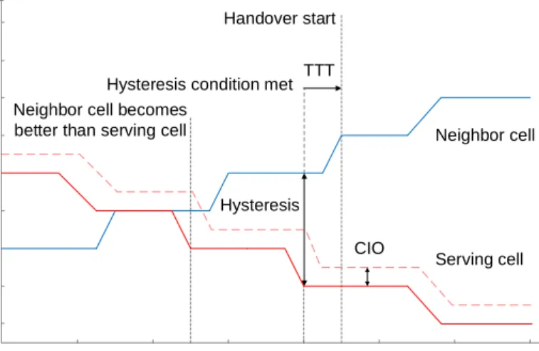
Among the different handover triggering procedures in LTE, we focus on Event A3, which is the main criterion to manage intra-LTE mobility. Event A3 is defined as the situation in which the UE perceives that a neighbor cell’s RSRP is better than the serving cell’s RSRP by a certain margin [24]. In order to reduce the ping-pong effect, measurements used to assess the event are averaged, hysteresis margins are introduced and the conditions must be met during the so-called TTT. Hence, the event entering condition is defined as
where RSRPnc and RSRPsc are the averaged reference signal power strengths of the neighbor
and the serving cell, respectively, while offset and hysteresis parameters cause the serving and neighbor cells to be more and less attractive, respectively [24]. The combination of both defines a net hysteresis margin that delays notification of the event to guarantee that the neighbor cell is now the dominant one. These values are used as a basis and can be modified to adapt the condition to a particular UE mobility status, for example, being reduced for a high-speed UE. Finally, the cell individual offset, or CIO, is a cell-specific parameter set by the serving cell for each of its neighboring cells. It is used for load management, since the higher its value, the more attractive the corresponding neighbor will be. The whole process can be appreciated in Figure 5a, which shows the trace of average RSRP measurements from the serving cell and a neighbor before and after a handover. On the other hand, Figure 5b illustrates the difference between the hysteresis margin and the TTT taken by each SON function.
B. SON Conflict
In order to explain the SON conflict, we implement MLB and MRO SON functions in a distributed manner. As previously introduced, both of them aim at adjusting the CIO, hysteresis and the TTT handover parameters for different purposes. The goal of MLB is to optimize the network quality of service (QoS) by evenly distributing the load among the different cells. On the other hand, the MRO aims at decreasing the number of radio link failures (RLFs) caused by too-early or too-late handovers.
Figure 6 shows that the two SON functions are implemented in a distributed manner and concurrently executed in a per-cell manner. In order to analyze the MLB-MRO SON conflict, we assume that the serving cell (cellA) is overloaded and its neighbor (cellB) has a lower load.
Therefore, cellA chooses its neighbor cellB to balance the load, and the action request is to
adjust the CIO, the hysteresis and TTT handover parameters. This way, the condition in Event A3 can be met by UEs close to the cell edge. Hence, several handovers will happen from cellA
Neighbor cell
Serving cell Hysteresis condition met TTT
Handover start Time (sec) 74 75 76 73 40 41 77 39 Neighbor cell becomes better than serving cell
R S R P ( d B m ) 72 36 37 38 42 43 78 79 80 Hysteresis CIO (a) Neighbor cell Serving cell Hysteresis condition met TTT
Handover start Time (sec) 74 75 76 73 40 41 77 39 Hystersis - CIO Hystersis - CIO_MRO Hystersis - CIO_MLB Neighbor cell becomes
better than serving cell
R S R P ( d B m ) 72 36 37 38 42 43 78 79 80 (b)
Fig. 5: Effect of the handover parameters. The figure on the left side depicts the perceived RSRP of serving cell and a neighboring cell by a UE, which crosses the border of the cells. By default, the algorithm uses a hysteresis margin of 3.0dB and a TTT of 256 ms. On the right, the MLB and MRO tune these values in order to achieve their own goals.
in cellA causing an increase in the RLFs rates and ping-pong effects. As a consequence, the
MRO SON function detects these metrics and tries to reduce them by requesting new changes in CIO, the hysteresis and TTT parameters. Since cellA is still overloaded, the MLB changes
Action request: Adjust CIO, Hysteresis and TTT parameters shorter to increase
the number of handovers
Find cell/UE candidate for load
balancing Mobility change Cell A Cell B X2 MLB MLB MME/GW MME/GW S1 (a)
Action request: Adjust CIO, Hysteresis and TTT parameters larger to prevent
too-early handovers RLF (Radio Link Failure) monitoring HO report Mobility Change Cell A Cell B X2 MRO MRO MME/GW MME/GW S1 (b)
Fig. 6: In the figure on the left side, the MLB aims at increasing the number of handovers by adjusting the CIOAB shorter to force UEs to handover to cellB, whereas in the figure on the
right side the MRO aims at decreasing the number of handovers by adjusting the CIOAB larger
to prevent too-early handovers.
C. Performance Indicators
Besides the UE measurement reports, which contain RSRP and RSRQ values coming from the serving and the neighboring cells, the data about the performance of each UE is also collected once it performs a handover. These metrics are chosen based on the objective of each SON function.
On the one hand, the main objective of MLB is to improve end-user experience and achieve higher system capacity by distributing user traffic across system radio resources. As a conse-quence, the load of a cell is measured in terms of the average physical resource blocks (PRBs) that can be allocated to the users and the average signal to interference plus noise ratio (SINR) of each cell. The number of bits at the physical layer, referred to as the transport block size (TBS), is chosen taking into account the data that need to be transmitted by a UE. The media access control (MAC) has to first decide on the modulation scheme that can be scheduled to the user and then check the physical resource grid for the availability of the resource blocks. Given this, the MAC can decide upon the modulation and coding scheme index and its TBS index taken from [25], and then decide the number of PRBs that can be allocated to the user (i.e., users are allocated a specific number of subcarriers for a predetermined amount of time).
On the other hand, the main objective of MRO is to guarantee proper mobility. So, in this case, RLF and the ping-pong effect are the performance metrics. RLFs may happen due to poor handover parameter settings, for example, a UE’s being forced to hand off too early to a cell and, as a consequence, failing to establish the new connection before a timer expires. The ping-pong effect happens when a new handover is performed back to the source cell right after a successful handover and a new handover is performed before a determined minimum time of stay. In both cases, the MRO will be activated.
At the beginning of every Transmission Time Interval (TTI), the system will detect the load level of every cell. If the resource usage is higher than a threshold, the MLB will be activated in that particular cell. On the other hand, if the system detects that RLFs occur in the serving
cell before, during or after a handover procedure, the MRO will be activated.
V. PERFORMANCE EVALUATION
As we stated earlier, in order to evaluate the performance of the proposed scheme, we consider the MLB-MRO SON conflict. We first present the simulation scenario and then the simulation results for this SON conflict.
A. Simulation Parameters
The proposed scheme is assessed by means of the 3GPP-compliant, full protocol stack, ns-3 LTE-Evolved Packet Core Network Simulator (LENA). The simulation setup is based on the assumptions for evaluating the SON conflict. We consider two sites of tri-sectored macro eNodeBs (i.e., three sectors per each site, resulting in six cells) regularly deployed with a 500 m inter-site distance and with UEs nonuniformly spread. A full-buffer traffic model, Transmission Control Protocol (TCP) and a Proportional Fair (PF) scheduler are considered. The PF works by scheduling a user when its instantaneous channel quality indicator is above its own average channel. The rest of the simulation parameters are described in Table I.
The LTE module of ns-3 has been used to evaluate the capacity of the proposed scheme and to solve the SON conflict proposed in Section IV. By doing this, we model not only the LTE radio access network, but also the corresponding core network, known as the Evolved Packet Core (EPC). In this sense, the EPC mode is used to provide end-to-end connectivity to the users. The EPC model also enables a direct connection between two eNBs (X2 procedure) to handover a UE from a source eNB to a target eNB, and the user average throughput is obtained by enabling the Radio Link Control (RLC) simulation output. Notice that in the LTE-EPC ns-3 network simulator, generally, there is no RLF (handling of radio link failure is not yet modeled), i.e., once the UE goes into a connected mode, it does not change its state during the simulation. In order to bypass this issue, we tune the handover by increasing the timers (e.g., the handover joining time). As a consequence, when a handover radio link failure occurs, handover timers will
TABLE I: Parameters.
LTE Value
Scheduler Proportional Fair
Transport protocol Transmission Control Protocol (TCP)
DL/UL traffic model Full-buffer
Layer link protocol Radio Link Control (RLC)
Mode Unacknowledged Mode (UM)
Carrier frequency 2GHz
Bandwidth 5MHz DL and UL
Number of PRBs 25
Transmission Time Interval (TTI) 1ms
Simulation time 200s
Macro cell scenario
Macro-cell sites 2
Number of cells 6
Number of UEs per cell in the range[7−37]
Number of UEs 108
Macro-cell Tx power 46dBm
UE Tx power 10dBm
Distance between adjacent
macro-cell sites 500m
Overloaded cell 1
TABLE II: Handover parameters.
Parameters Value
RSRP range 0-97 dBm
CIO values 0-30 dB
Hysteresis values 0-15 dB
TTT 13 first valid values (all in ms) [24]
Mobility Random Walk Mobility
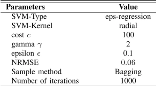
TABLE III: Bagged-SVM parameters.
Parameters Value SVM-Type eps-regression SVM-Kernel radial costc 100 gammaγ 2 epsilon 0.1 NRMSE 0.06
Sample method Bagging
Number of iterations 1000
indicate such situation in a natural manner. In the case that a UE goes very far away from the eNB, schedulers just stop assigning resources to that UE, and once it comes back, allocations start again. As a result, we consider that a UE detects an RLF when its channel quality indicator
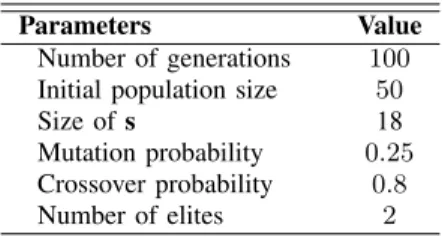
TABLE IV: GA parameters.
Parameters Value
Number of generations 100
Initial population size 50
Size ofs 18
Mutation probability 0.25
Crossover probability 0.8
Number of elites 2
is equal to zero, and the MAC traces of that UE will be zero, meaning, the UE is out of range during that period of time. The handover parameters are described in Table II, and the ML and genetic algorithm parameters are described in Tables III and IV.
B. Simulation Results
We present the simulation results that allow a performance comparison between two different schemes:
1) The MLB and MRO are independently executed, and they tune the CIO, hysteresis and TTT handover parameters to achieve their own objectives.
2) Proposed scheme: The self-coordinator framework is activated to avoid the MLB-MRO SON conflict (BDA-NSGA-II).
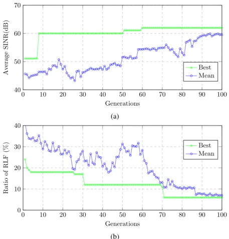
In order to evaluate the performance of the MLB-MRO SON functions, each one is executed independently. We implement both of them by taking advantage of genetic algorithms. For this scheme, the metrics are the average SINR to evaluate the performance of the MLB SON function, and the RLF rate for the case of the MRO SON function. We define the RLF rate as the number of RLFs divided by the total number of handovers performed during a predefined time window. Figures 7a and 7b show the fitness value of the best individual found in each generation (Best) and the mean of the fitness values across the entire population (Mean). We observe that, the chromosome tends to get better as generations proceed. Figure 7a depicts the time evolution of the average SINR in the scenario during the evolution of the genetic algorithm. We observe that, as the generations proceed, the MLB SON function is able to find the configuration of the
0 10 20 30 40 50 60 70 80 90 100 40 50 60 70 Generations Av erage SINR(dB) Best Mean (a) 0 10 20 30 40 50 60 70 80 90 100 0 10 20 30 40 Generations Ratio of RLF (%) BestMean (b)
Fig. 7: Evolution of the performance when MLB and MRO functions are independently executed.
vector with handover parameters that maximize the value of SINR. Similar behaviors can be appreciated in Figure 7b, where the figure shows the evolution of the genetic algorithm in terms of the ratio of RLF.
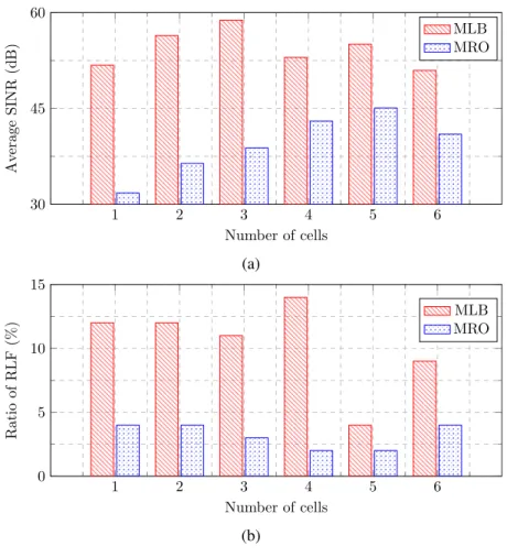
Figures 8a and 8b show the performance of each cell in the network as a consequence of the actions taken by MLB and MRO SON functions. In Figure 8a, we observe that the actions taken by the MLB function yield higher values of SINR. This is because the number of overloaded cells has been reduced by choosing appropriate neighbors to balance the load. The action that is requested by the MLB function is tuning the values of the CIO, the hysteresis margin and the TTT to promote handovers. However, due to the new consecutive handovers, executed within a short period of time, the ratio of RLF increases (see Figure 8b). We observe opposite behaviors
1 2 3 4 5 6 30 45 60 Number of cells Av erage SINR (dB) MLB MRO (a) 1 2 3 4 5 6 0 5 10 15 Number of cells Ratio of RLF (%) MLB MRO (b)
Fig. 8: MLB-MRO performances.
in case of the MRO SON function, which decreases the ratio of RLF in each cell, but also decreases the values of SINR in each cell.
In the following paragraphs, we analyze the performance results for the proposed scheme. As we stated in Section V, the metrics that have been considered are the average number of PRBs allocated to each user and the MLB and MRO objective functions, average SINR and RLF and ping-pong ratios, respectively.
As we already explained in Section III, once we extract the most relevant information from the mobile network, the next step is to obtain the network performance prediction model. To do that, we determine the SVM tuning parameters (see Table IV) prior to fitting the model,
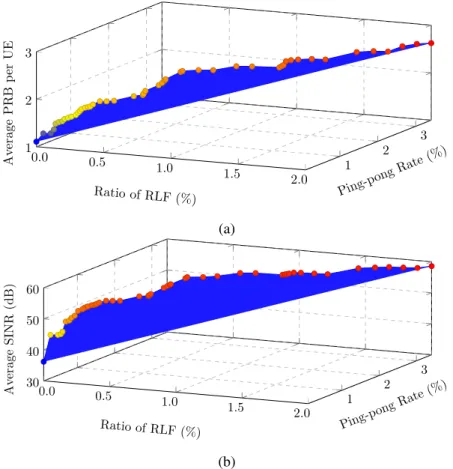
and then we fit the training data. The SVM regression model is run several times, each with a different subset of training samples. Finally, in order to evaluate the accuracy of the predictions, the performance of the learned function is measured on the test set, resulting in 94%prediction accuracy, which is expressed in terms of (1-NRMSE)×100, where NRMSE is the normalized RMSE. Then, the network performance prediction model is fed into the NSGA-II, which finds the best configuration of handover parameters for each cell. The first step when solving a multi-objective problem is to get a handle on the feasible region. Figures 9a and 9b capture the whole spectrum of the Pareto front considering the average number of PRBs and the average SINR respectively. Note that the Pareto front has four dimensions, one for each of the performance metrics to optimize: the radio link failure rate, the ping-pong rate, the average number of physical resource blocks allocated to UEs and the average SINR. Hence, in order to provide an insightful representation, we have provided two 3-D projections (Figures 9a and 9b). Each figure represents three of the objectives: the ratio of RLFs, the ping-pong rate and the average number of PRBs per UE in case of Figure 9a and the average SINR in Figure 9b. If there were a single point that minimizes these objectives, it would be the solution; but often, there are different optimal points for each objective. These are represented on the top of the figure and they determine the Pareto front. Any point on this front is a non-dominated or “Pareto optimal” solution. By moving along the curve, it is possible to prioritize the minimization of RLFs and ping-pong rate at the expense of the SINR, or vice versa, but we cannot improve all three of them at once, and the blue shaded region is the feasible region. However, any point in the feasible region that is not on the Pareto front is not a non-dominated solution. Each objective can be improved with no penalty to the other. From these figures, we observe that the proposed scheme, referred to hereafter as BDA-NSGA-II, gives us the set of points that provides the best performance of conflicting SON functionalities, i.e., by predicting the performance metric based on the historical data collected from the network, we are able to find the operating point that provides the best performance trade-off. Moreover, Figures 10a-10c represent the parameter space. That is, each bin represents
0.0 0.5 1.0 1.5 2.0 1 2 3 1 2 3 Ratio of RLF (%) Ping-p ongRate (%) Av erage PRB p er UE (a) 0.0 0.5 1.0 1.5 2.0 1 2 3 30 40 50 60 Ratio of RLF (%) Ping-p ongRate (%) Av erage SINR (dB) (b)
Fig. 9: Objective space considering the average number of PRBs per UE, the ratio of RLF and ping-pong rate objectives (left side), and the average SINR, the ratio of RLF, and ping-pong rate objectives (right side).
the ratio (%) of the values of the CIO, hysteresis and TTT on the Pareto front. In order to avoid misunderstanding due to the diversity in CIO and hysteresis values, we define three different indicators for Figures10a and 10b. Please note that the meaning of the x-axis labels are indicated in Table V. In order to calculate the ratios, we consider the frequency distribution of the values of each handover parameter chosen by each SON function and the proposed scheme in the last population of solutions. Then, for each value we calculate the percentage as noccurrences
psize ×100,
where noccurrences is the number of times that each value has been selected in the solutions, and
psize is the size of the population itself.
TABLE V: CIO and Hysteresis x-axis indicators.
CIO Hysteresis
Low [0, 10] [0, 5]
Medium (10, 20] (5, 10] High (20, 30] (10, 15]
highest rate. On the other hand, for the TTT, which delays handover execution, just 8 values out of the 16 possibilities defined by the 3GPP are found, with 128 ms being the most likely one. It is important to note that all the solutions in the Pareto front are non-dominated and constitute a global solution to the SON conflict in the form of trade-off. That is to say, the tool provides a set of solutions, and the operator must choose one or another depending on the objective to be prioritized. It is a usual practice to define thresholds for each of the performance metrics and to choose a solution respecting all of them (or at least the closest one). In this particular example, we choose one of the solutions having an RLF ratio < 1%, ping-pong rate
<1%, average SINR>15 dB and the average number of allocated PRBs >2. Figure 11 shows the Cumulative Distribution Function (CDF) of the cell average throughput. From this figure, we observe that our proposed scheme is able to find the operating point that provides the best performance trade-off.
VI. CONCLUDING REMARKS
In this paper, we have addressed the issue of SON conflict. In particular, we focus on the SON conflict that results from the concurrent execution of multiple SON functions. The main contribution of this work is to present a framework that is able to take advantage of big data analytics, i.e., we exploit the huge amount of data already available in the network to predict future performance. We build a prediction model based on historical UE measurements, and we apply regression analysis techniques to predict network performance. The built model is then used as an input of multi-objective evolutionary algorithm to solve the potential conflicts by finding a set of solutions that satisfy the objectives at an acceptable level without being dominated by any other solution.
Low Medium High 0.0 0.2 0.4 0.6 0.8 1.0 CIO Values Ratio(%) BDA-NSGA-II MRO MLB (a)
Low Medium High
0.0 0.2 0.4 0.6 0.8 1.0 Hysteresis Values Ratio(%) BDA-NSGA-II MRO MLB (b) 64 128 160 256 320 512 640 1024 0.0 0.2 0.4 0.6 0.8 1.0 TTT Values Ratio(%) BDA-NSGA-II MRO MLB (c)
Fig. 10: Ratio of the handover parameters across the Pareto front.
To evaluate the performance of the proposed scheme, we focus on the MLB-MRO SON conflict. The simulation results demonstrate the ability of the proposed scheme to solve conflicts
0.00 0.05 0.10 0.15 0.20 0.25 0.0 0.2 0.4 0.6 0.8 1.0 Average THR(Mbps) CDF BDA-NSGA-II MLB MRO
Fig. 11: CDF of the average throughput values in the whole network.
based on a prediction of network performance, which is obtained from a proper analysis of UE measurements. As a result, the proposed scheme learns from past experience to predict network performance according to the target of each SON function and then solve the conflict based on non-dominated solutions.
ACKNOWLEDGMENT
This work was supported by the Spanish National Science Council and ERFD funds under TEC2014-60258-C2-2-R and TEC2017-89429-C2-2-R projects.
REFERENCES
[1] 3GPP, “Evolved Universal Terrestrial Radio Access Network (E-UTRAN); Self configuring and self optimizing network uses case and solutions (Release 9),” 3GPP, TR 36.902, v9.2.0, 2009.
[2] J. Johansson, W. A. Hapsari, S. Kelley and G. Bodog, “Minimization of drive tests in 3GPP release 11,” IEEE Communications Magazine, vol. 50, no. 11, pp. 36–43, November 2012.
[3] 3GPP TSG SA WG5 (Telecom Management) Meeting 85, “Study of implementation alternative for SON coordination,” 3GPP, TSG S5-122330, 2012.
[4] Z. Altman, M. Amirijoo, F. Gunnarsson, H. Hoffmann, I. Z. Kovcs, D. Laselva, B. Sas, K. Spaey, A. Tall, H. van den Berg and K. Zetterberg, “On design principles for self-organizing network functions,”2014 11th International Symposium on Wireless Communications Systems (ISWCS), pp. 454–459, August 2014.
[5] K. Deb, A. Pratap, S. Agarwal and T. Meyarivan, “A fast and elitist multiobjective genetic algorithm: NSGA-II,”IEEE Transactions on Evolutionary Computation, vol. 6, no. 2, pp. 182–197, April 2002.
[6] T. Bandh, H. Sanneck and R. Romeikat, “An experimental system for son function coordination,”2011 IEEE 73rd Vehicular Technology Conference (VTC Spring), pp. 1–2, May 2011.
[7] J. Moysen and L. Giupponi, “Self-coordination of parameter conflicts in D-SON architectures: A Markov decision process framework,”EURASIP Journal on Wireless Communications and Networking, vol. 2015, no. 1, p. 18 pages, March 2015. [8] J. Chen, H. Zhuang, B. Andrian and Y. Li, “Difference-based joint parameter configuration for MRO and MLB,”2012
IEEE 75th Vehicular Technology Conference (VTC Spring), pp. 1–5, May 2012.
[9] P. Mu˜noz, R. Barco and I. de la Bandera, “Load balancing and handover joint optimization in LTE networks using fuzzy logic and reinforcement learning,”ELSIVER Computer Networks, vol. 76, pp. 112–125, January 2015.
[10] O. Iacoboaiea, B. Sayrac, S. Ben Jemaa and P. Bianchi, “SON Coordination for parameter conflict resolution: A reinforce-ment learning framework,”2014 IEEE Wireless Communications and Networking Conference Workshops (WCNCW), pp. 196–201, April 2014.
[11] C. Szepesv´ari, “Algorithms for reinforcement learning, ser. G - Reference information and interdisciplinary subjects series,” Morgan and Claypool, 2010.
[12] N. Baldo, L. Giupponi and J. Mangues-Bafalluy, “Big data empowered self organized networks,”20th European Wireless Conference, pp. 1–8, May 2014.
[13] A. Imran, A. Zoha and A. Abu-Dayya, “Challenges in 5G: How to empower SON with big data for enabling 5G,”IEEE Network, vol. 28, no. 6, pp. 27–33, November 2014.
[14] J. Moysen, L. Giupponi, and J. Mangues-Bafalluy, “A mobile network planning tool based on data analytics,” Mobile Information Systems, Hindawi, vol. 2017, February 2017.
[15] J. Moysen, L. Giupponi, N. Baldo and J. Mangues-Bafalluy, “Predicting QoS in LTE HetNets based on location-independent UE measurements,”2015 IEEE 20th International Workshop on Computer Aided Modelling and Design of Communication Links and Networks (CAMAD), pp. 124–128, September 2015.
[16] J. Moysen, L. Giupponi and J. Mangues-Bafalluy, “On the potential of ensemble regression techniques for future mobile network planning,”2016 IEEE Symposium on Computers and Communication (ISCC), pp. 477–483, June 2016.
[17] K. Van Moffaert and A. Now´e, “Multi-objective reinforcement learning using sets of Pareto dominating policies,” The Journal of Machine Learning Research, vol. 15, no. 1, pp. 3483–3512, January 2014.
[18] T. G. Dietterich, “An experimental comparison of three methods for constructing ensembles of decision trees: Bagging, boosting and randomization,”Machine Learning, vol. 40, pp. 139–157, August 2000.
[19] V. N. Vapnik,The Nature of Statistical Learning Theory. New York, NY, USA: Springer-Verlag New York, Inc., 1995. [20] E. M. Jordaan and G. F. Smits, “Estimation of the regularization parameter for support vector regression,”on Proceedings
of the International Joint Conference Neural Networks (IJCNN), vol. 3, pp. 2192–2197, 2002.
[21] N. Cristianini and J. Shawe-Taylor,An Introduction to Support Vector Machines and Other Kernel-based Learning Methods. Cambridge University Press, 2000.
[22] A. Smola and B. Sch¨olkopf, “A tutorial on support vector regression,”Statistics and Computing, vol. 14, no. 3, pp. 199–222, August 2004.
[23] J. H. Holland,Adaptation in Natural and Artificial Systems. Cambridge, MA, USA: University of Michigan Press, Ann Arbor, 1975.
[24] 3GPP, “Technical Specification Group Radio Access Network; Evolved Universal Terrestrial Radio Access (E-UTRA); Radio Resource Control (RRC); Protocol Specification (Release 10),” 3GPP, TS 36.331, v10.7.0, 2010.
[25] ——, “Technical Specification Group Radio Access Network; Evolved Universal Terrestrial Radio Access (E-UTRA); Physical layer procedures (Release 10),” 3GPP, TS 36.213, v10.2.0, 2011.