Does Financial Development Lead to Trade Liberalization?

Does Financial Development Lead to Trade Liberalization?*

2000 09 10

Helena Svaleryd+ and Jonas Vlachos++

It has long been argued that trade restrictions can be motivated by insurance considerations in the absence of full risk diversification. Recent theoretical research suggests that markets for risk can alleviate resistance to reform and protectionist lobby group pressure. We empirically address the hypothesis that institutions reducing risk can facilitate liberal trade policy. Our results reveal a robust positive relationship between openness to trade and the development of domestic and international financial markets.

JEL Classification: F13; G20

Keywords: Financial markets; Trade policy; Panel data

*

We thank Marcus Asplund, Tore Ellingsen, Lars Frisell, Almas Heshmati, Fredrik Heyman, Torsten Persson, two anonymous referees and seminar participants at the Stockholm School of Economics and Stockholm University for helpful suggestions and Mark Blake for editorial assistance. Dani Rodrik and Romain Wacziarg have generously shared their data with us.

+

Department of Economics, Stockholm University, 106 91 Stockholm, Sweden. Email: [email protected].

++_{Corresponding author:}

Department of Economics, Stockholm School of Economics, Box 6501, 113 83 Stockholm, Sweden. Email: [email protected].

1. Introduction

It has long been argued that trade restrictions can be motivated by insurance considerations in the absence of full risk diversification. See for example Corden [1974], Hillman [1977], Cassing [1980], Newbery and Stiglitz [1984], Eaton and

Grossman [1985], Cassing et al. [1986].1 It follows that the development of

institutions for risk diversification, e.g. financial markets, might reduce barriers to trade. Given the abundance of theoretical models, it is surprising that no empirical work has brought this hypothesis to the data. In this paper, we address the issue empirically and show that there exists a positive relation between openness to trade and proxies for the degree of financial sector development in a broad panel of countries.

International trade brings about substantial changes in competition, technology, prices of intermediary and final goods, and in the long run even in factor endowments and the institutional features of a society. The exact outcome of trade liberalization for different individuals is therefore uncertain. Rodrik [1998] provides evidence that openness to trade also increases the permanent degree of income volatility in an economy.2 The theoretical papers mentioned above argue that trade barriers can be welfare enhancing if private markets fail to pool such risks. Feeney and Hillman [1998] explicitly demonstrate how asset market incompleteness can affect trade policy in a lobby group model. In their model, the degree portfolio diversification determines the protectionist lobbying effort conducted by owners of sector specific capital. If risk can be fully diversified, special interest groups have no incentive to lobby for protection and free trade will prevail.

In the light of this literature, we ask the question whether institutions allowing for better insurance possibilities and risk diversification within a country facilitate the removal of trade barriers. In particular, we investigate whether the development of domestic financial markets is systematically related to trade policy. Moreover, since openness to trade increases aggregate income volatility, we expect international

1

Dixit [1987, 1989ab] is a dissenting voice in this literature. When explicitly modeling the reasons behind the absence of insurance markets, he finds the scope for government intervention to be limited.

2

Traca [2000] shows theoretically that we have reasons to expect trade to increase income volatility. Further empirical evidence for this view is given in Gottschalk and Moffit [1994], and Ghosh and Wolf [1997].

financial integration to reduce the demand for trade protection. This hypothesis is also brought to the data. The expected positive relation between financial development, both domestic and international, and openness to trade appears clearly in both a cross-country and a panel data setting. Simple causality tests indicate that causality runs both from trade to financial development and in the opposite direction. However, instrumental variable techniques reveal an exogenous effect of financial markets on trade.

This paper is organized as follows. Section 2 provides a more extensive theoretical and empirical motivation for the study. Section 3 outlines the empirical methodology, while section 4 describes the data. Especially how we measure trade policy and the development of the financial sector. Section 5 presents the results and section 6 concludes.

2. Theoretical and empirical motivation

As mentioned in the introduction, there are a number of papers dealing with trade policy as an insurance device, all set within a social planner framework. Feeney and Hillman [1998], however, provide a positive theory of trade policy as income insurance. Specifically, they model a two-sector economy with perfectly negatively correlated productivity shocks, which determine which sector will be exporting and import competing. Ex post the import competing sector can choose to lobby for protection and policy makers respond by implementing a tariff. The tariff increases the price for the import-competing good but it also induces a consumption distortion in the economy thereby lowering aggregate welfare. In the standard case when no portfolio diversification is possible, the equilibrium tariff will always be positive since the income gain from lobbying is larger than the consumption distortion for the import competing sector.

Next domestic asset markets are introduced into this framework. Suppose that before the uncertainty regarding productivity is revealed, specific factor owners can trade in the asset markets. In the case when asset markets work without friction, the incentive for lobbying disappears since specific factor owners will optimally hold a fully diversified portfolio with specific capital from both sectors and therefore only care about aggregate welfare. Suppose instead that the agents can only trade with a subset

of capital. They may then be unable to reach a perfectly pooled equilibrium. The extent of lobbying and consequently tariffs will be determined by the difference between the income gain and the consumption distortion. Compared to the model without any trade in sector-specific capital, the limited access to capital markets reduces the payoff from protectionist policies. Thus, the degree of asset market incompleteness affects the lobby pressure for the imposition of tariffs and consequently how liberal a country’s trade policies will be. Regardless of how susceptible the political sector is to private demand for protection, this effect will always be present. Given this setup, the empirical prediction would be a causal effect from financial development to trade liberalization. Another possibility is that the demand for financial services increases when the volatility of income goes up. In this case causality would run from openness to financial development.

The main focus of the Feeney-Hillman model is on domestic diversifiable risk and the functioning of domestic financial markets. The productivity shocks that hit the two sectors are perfectly negatively correlated implying that the risk can be domestically diversified.3 The assumption that a significant share of the risk facing the agents can be domestically diversified, receive support in studies of output shocks and volatility. Ghosh and Wolf [1997] use US data to show that shocks to output growth in a particular industry in a particular state is mainly driven by shocks to the sector, and that these shocks are not (much) correlated across sectors. Hence there is scope for risk diversification between industries within a country using domestic financial markets. Using international data, Clark and Shin [2000] provide further support for this view by showing that the main source of variation in output and employment for an industry in a country is due to shocks to that industry in that country (as opposed to shocks common to the whole country or industry). By showing that shocks to the traded goods sector are larger than shocks to the non-traded goods sector, Ghosh and Wolf also provide indirect evidence that trade increase the volatility of output, i.e. support for the underlying assumption in the models mentioned in the beginning of this section.

3

In some cases, access to international asset markets can reduce lobbying pressure in the Feeney-Hillman model. For this to happen, an asymmetry of assets that can be traded must be present between

The higher volatility of the tradable sector, compared to the non-tradable sector, is given a theoretical explanation in Traca [2000].4 In his model, productivity shocks hit both sectors. The tradable sector is also subject to price shocks, uncorrelated to the productivity shocks. When shocks hit the non-traded goods sector, prices move to offset the volatility of aggregate income. Since world market prices are given, no such offsetting mechanism is at work in the traded goods sector. Hence volatility in this sector is higher.

Although the main focus of this paper is the impact of domestic financial development on trade policy, it is obvious that an international dimension exists as well. If trade raises aggregate risk, as Rodrik [1998] argues, it is not possible to diversify this risk in purely domestic financial markets. Therefore, the amount of international risk sharing should also have a positive impact on openness to trade. In addition, Feeney and Hillman [2000] observe that internationally open financial markets eliminate of reduce the interest in strategic trade policy. This being said, the literature on international risk sharing indicates that this effect is likely to be small. When summarizing the evidence, Lewis [1995] and Tesar [1995] find that the amount of consumption smoothing that take place internationally is limited and that this amount is quite persistent over time.5 Moreover, there is a strong ‘home-bias’ in equity holdings, suggesting that portfolios are not optimally diversified.6 One reason for this could be the blurred distinction between international and domestic financial markets. Due to the presence of internationally active corporations and the cross-listing of companies, it is possible that international diversification can be achieved within the domestic market. It is clear that whatever measures we use to capture the degree of domestic financial development will also capture this effect.

Another issue regarding international financial integration is concerned with the timing of liberalization events. The Feeney-Hillman model suggests that financial

sectors. If we interpret the share of tradable capital as the degree of financial development, the

assumption of asymmetries between sectors is quite odd.

4

Traca cites empirical evidence by Gottschalk and Moffit [1994] to motivate his model.

5

The last point is important because if international risk sharing is constant over time, this effect will be captured by the country specific fixed effects when running panel regressions.

6

Stulz [1999] finds more recent evidence that globalization has so far had quite a limited impact on the cost of capital to firms. Kraay et al. [2000] show that countries’ foreign asset positions have been very persistent over time and have mainly taken the form of loans rather than equity during the 1966-1997 period. Both these papers indicate that international capital markets are not yet well integrated.

integration should precede trade liberalization. Generally, however, trade liberalization seems to proceed or be simultaneous with international financial liberalization.7 In practice, it is difficult to separate trade and financial liberalization from each other. As shown by Tamirisa [1999], capital controls can effectively work as an impediment to trade. Thus, measures of financial openness, rather than explaining trade policy, may be part of what we wish to explain. Since trade and financial liberalization can be part of the same policy, questions concerning the timing between the two types of events may hence even be impossible to answer.8

3. From Theory to Estimation

There are, of course, other determinants of trade policy besides the concern for insurance. The optimal tariff argument makes it clear that countries, (economically) large enough to affect international goods prices can increase their welfare by the introduction of a tariff. In a related vein, Alesina and Wacziarg [1998] argue that the cost of self-sufficiency is lower for large than for small countries. Countries with large markets should therefore be less open to trade than countries with small domestic markets. As the demand for variety in the choice of goods is likely to increase with wealth, per capita GDP is another probable determinant of trade policy.9 This leaves us with the following basic trade policy equation to estimate:

Trade Policy = f(Market Size, GDP, Financial Development)

Since the institutional environment is roughly the same for all sectors within a country, and risk diversification is essentially an inter-sector activity, the natural level of comparison is between countries. It is of course possible that the need and the opportunities for risk diversification differ between industries. However, since it is unclear in what way industries differ, we argue that the most suitable approach is to

7

We thank an anonymous referee for making this point.

8

There are of course other factors that can explain financial liberalization. One is that the gains from the removal of capital restrictions can increase after an increase in trade since the volume of

international transactions has gone up. Another reason (not related to trade) is that governments running deficits might want to free capital movements in order to get access to international credit more cheaply.

9

The inclusion of per capita GDP in the trade policy equation can be motivated by other arguments as well: Industrial specialization and dependence on imported intermediate goods are just some factors likely to increase with GDP.

use country level data. Thus, we analyze how aggregate measures of financial development affect the aggregate trade policy choices made in a country.

Due to the level of aggregation, it is neither possible to discriminate between different sources of uncertainty, nor to be explicit about the mechanism that causes financial development to affect openness to trade. What is possible, however, is to control both for aggregate risk caused by openness and for aggregate income uncertainty. This is of importance since domestic asset markets cannot help diversifying aggregate risk.

A standard cross-section approach has the disadvantage of being a static approach to the essentially dynamic problem of financial development and trade policy. To allow for a time dimension, we make extensive use of panel data. Panel data has a number of advantages compared to both cross-section and time-series analysis, the most obvious being the ability to control for time and country specific fixed effects. In addition, the panel approach allows us to undertake causality tests not possible in a cross-section setting.

4. Data

The panel in this study is constructed for the years 1960-1994. To smooth short-term fluctuations, and to fill gaps in the series, all time varying variables are averages over five year periods. The selection of countries is based on the widely used Barro-Lee [1994] data set, which contains data for 138 countries. Data availability restricts the sample for some regressions to around 80 countries (for more details on the data, see Table A1 in the Appendix). When running panel regressions, we first remove countries for which one or more variables are only available for one (or no) time periods. This procedure allows us to make better comparisons between fixed and random effects estimations. We also check for outliers and remove Hong Kong and Singapore as these countries display an extreme degree of trade, which largely consists of transit trade. We now turn to the more serious problem of how to measure trade policy and financial sectors.

4.1 Measuring trade policy

There is a huge literature discussing the pros and cons of different aggregate measures of the restrictiveness of trade policy (see for example Harrison [1996], Anderson and

Neary [1998]). The conclusion to be drawn from these studies is that no fully satisfactory measure is available. For our purpose, the measures should be objectively comparable across countries and time. These requirements severely restrict the number of measures at hand.

A popular direct measure of trade policy is the Sachs-Warner [1995] index. In their study of the period between 1950-94, a country is judged as open when it does not not fulfill any single one of the following criteria: (i) Average tariffs are higher than 40%, (ii) non-tariff trade barriers cover more than 40% of imports, (iii) the economic system is considered socialist, (iv) major exports are monopolized by the state, (v) the black market exchange rate premium exceeded 20%. The fraction of years between 1950-94 when the country is judged as open is then used to construct the index. A natural criticism of this index is that the different criteria might not be equivalent when evaluating the protectionist impact of trade policy. Yet another problem is that the index only considers the discrete nature of trade policy and not the degree of restrictiveness. Despite these criticisms, the index is useful since it attempts to handle the problem of aggregating and combining different aspects of trade policy coherently across countries and time.

The second indicator of trade policy to be used is openness, measured as the ratio of the sum of imports and exports to GDP. Openness itself is not a measure of trade policy since trade is determined by other factors than policy. Lee [1993] constructs a simple measure of free trade openness, which controls for distance to the world’s major trading economies and land area. The main advantage compared to the incidence measures is that all relevant trade restrictions are captured in a single,

aggregate measure. The most obvious shortcoming here is the hypothetical

counterfactual under free trade, making the measure sensitive to misspecifications of the trade equation. Despite these limitations, we will follow Lee and control for structural features of the economy and use trade share to GDP as a measure of trade policy (OPEN in this paper).10

10

We have experimented using an “effective tariff”-measure, defined as tariff revenue divided by the value of imports. This measure has some severe drawbacks. Using population, foreign direct

investment, land area, population density, per capita GDP, measures of financial development, and regional dummies as explanatory variables of our effective tariff measure, we basically find that GDP

4.2 Measuring financial development

The purpose of the paper is to investigate whether the financial system, in its role as an insurance mechanism, is correlated with trade openness. Thus, we need a measure describing the financial systems ability to hedge, diversify, and pool risks.

The possible proxies for financial development can be divided into three different categories: The size of financial sector; the financial systems ability to allocate credit; and the real interest rate. Since the real interest is largely affected by macroeconomic factors, it will not be used in this study. A general problem with size based measures is that the size of the financial sector does not necessarily measure its ability to diversify risk.

The most popular measure for size of financial sector is the ratio of liquid liabilities to GDP, labeled LLY in this paper. A potential problem with this measure is that it can be too high in countries with undeveloped financial markets, since no other value-keeping asset than money exists. To allocate credit is a major function of the financial sector, especially the banking industry. Proxies focusing of the financial system’s ability to allocate credits have been developed by for example King and Levine [1993ab]. Since we are interested in the financial system’s ability to diversify private sector risk, we will use credit issued to private enterprises divided by GDP, and label it DC.

Another kind of measure focuses on the stock market. Levine and Zervos [1998] measure stock market capitalization by the value of listed companies on the stock market as share of GDP in a given year (here labeled MCAP). Although large markets do not necessarily function effectively, many researchers use capitalization as an indicator of stock market development. Compared to the other measures, MCAP is intuitively better related to the underlying idea of portfolio diversification than LLY and DC. Unfortunately, this variable is not available prior to 1975, and the number of countries for which MCAP is available is also more limited than for LLY and DC.

and population are significant, but the explanatory power of these regressions is very low. The results from these regressions are not presented.

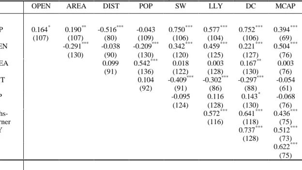
The correlations between LLY, DC, MCAP, and GDP (among other variables) are presented in Table A2.11

4.3 Measuring the possibilities of international risk-sharing

The IMF annually summarizes the restrictions on international capital markets that

each country imposes in their report Exchange Arrangements and Exchange

Restrictions. These indicators take the number one if a certain restriction is imposed and zero otherwise. Although these binary indicators are, they are the only available measure for a wide range of countries over time (we have data between 1967-1993). Moreover, they have been found to have significant explanatory power on international consumption risk sharing (Lewis [1996]), thus making them suitable for our purposes. In order to account for the differences in the degree of restrictiveness between countries, the simple annual average of four indicators is calculated and

labeled CAPCONT.12 These annual averages are then converted into five-year

averages in order to fit the rest of the data.

5. Results

Now we are ready to formulate the specifications we would like to estimate. Theory predicts that better developed financial markets will reduce risk and lead to less trade protection, even when controlling for other determinants of trade policy. This prediction is given support in the data.

5.1 The Sachs-Warner index

We begin by looking at the Sachs-Warner index. Given the discussion in Section 2 we use land area and population as proxies for country size and GDP per capita as a measure of wealth. According to theory, the size proxies should have a negative effect and GDP a positive effect on openness. Moreover, we include dummies for geographical region (OECD, East Asia, Latin America and Sub-Saharan Africa) and proxies for financial development in the regression. In line with our hypothesis, we

11

In Table A2 the correlations in the 1990-94 cross section are presented. The results are essentially unchanged when considering the full sample of observations.

12

The indicators are ‘Bilateral payments’, ‘Restrictions for payments on capital transactions’,

‘Restrictions for payments on current account transactions’, and ‘Proscribed currency/payment arrears’. See Lewis [1996] for a thorough discussion of the data. Using alternate versions of this index does not affect the results to any significant degree. However, when using the widest measure (capital

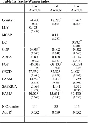
expect the proxies for financial development to enter with a positive sign. Since the Sachs-Warner index is an aggregate index based on the fraction of years a country has been open since 1950, we can not take the time variation of the variables into account. Since it is not obvious which time period to use in OLS regressions, we use the average of the explanatory variables to estimate the following equation:

Sachs-Warneri = α + β1AREAi + β2POPi + β3GDPi + β4FDi +β5Regioni + εi

where FDi is one of our measures of financial development. The results from the

estimations are presented in Table 1. The coefficients on LLY and DC are positive and significantly different from zero, as expected. MCAP, however, is not significant on conventional levels. One possible explanation is that the MCAP sample mainly includes OECD countries, which score high on the index. Per capita GDP is positive but only significant in one specification. Population enters, as expected, negatively into the regressions although not always statistically significant. The other proxy for size – area is never significant. Adding foreign direct investments as a control variable (not reported here) does not affect the results. Due to the construction of the index, the interpretation of the coefficient values of 0.43 and 0.38 is not fully clear. In the full sample of observations, the medians of LLY and DC are around 29 and 22, with standard deviations of 24 and 26, respectively. The median of the Sachs-Warner index is 20. An increase in LLY or DC by about one standard deviation (25 percentage points) would yield an increase in the index by 10. For a country around the median of the Sachs-Warner scale (New Zealand and Mexico), an increase of 10 is equivalent to getting ahead of 5 countries in the openness ranking. Thus, the results indicate a positive relationship between openness and financial development. The proxies for financial development are statistically significant in two out of three specifications.

As discussed in Section 2, we would like to control for international financial openness. The measures at hand, however, partly overlap with the Sachs-Warner index and should thus not be included in the regressions. However, if we nevertheless include the measure CAPCONT, the results remain virtually unchanged.

transactions) by itself, this variable loses its significance. Since most countries have some restrictions on international transactions, this should be of no surprise.

[Table 1A here]

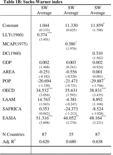
Since the Sachs-Warner measure is constructed as an average over the period 1950-1994 it is not clear how one would go about to investigate the question of causality. In Table 1B we re-estimate the specifications in Table 1A, but instead of using the average of the financial markets proxies we use their initial value. The rationale is that if the causality runs from financial markets to openness, the initial level of financial market development should be a determinant of a country’s future openness. The results show that the initial level of LLY and MCAP can explain the degree of openness. However, DC is no longer statistically significant. At least the results do not contradict the prediction that the initial level of financial market development affects the country’s openness for trade.

[Table 1B here]

5.2 Openness: Cross-sectional results

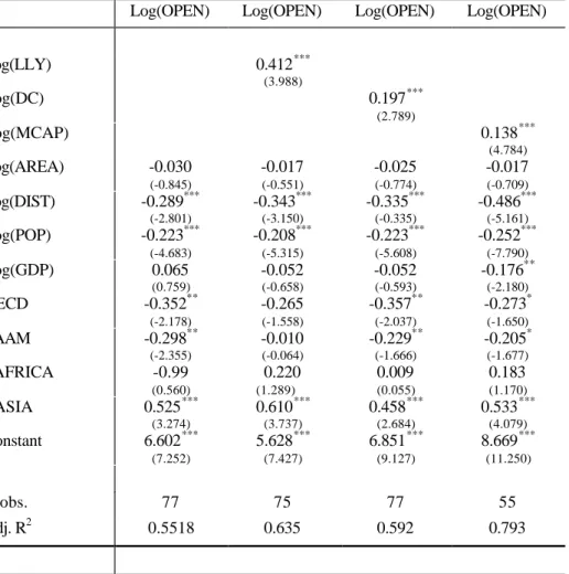
The other approach chosen to investigate whether financial markets affect trade policy is to use the direct measure of trade, i.e. OPEN. Actual trade is not a measure of trade policy therefore we must control for structural factors such as population and area. Not only does country size affect trade policy it also affects the country’s propensity to trade. This assumption is based on gravity models, which show that, everything else equal, large countries will tend to trade less than smaller ones. GDP per capita is included given the reasons presented in section 3. Further, high transportation costs are likely to decrease trade by making it less profitable. We use our aggregate distance measure as a proxy for transportation cost. We also include regional dummies. This gives us the following baseline cross-section specification:

OPENi = α + β1AREAi + β2POPi + β3DISTi + β4GDPi + β5FDi + β6Regioni + ει

The results from cross-sectional regressions on 1990-94 data are presented in Table 2. We estimate the baseline regression both with and without the inclusion of measures of financial development. In the presented regressions all variables are in logs. We can motivate a log specification on theoretical grounds: It is reasonable to assume that

the risk reducing effect is more important when starting from a low degree of

financial development.13 The results, however, are not contingent on the log

specification. In the baseline openness equation (column 2), population and distance indeed come out with the expected negative sign. Moreover, the proxy for financial markets, LLY, is statistically significant and positive as predicted by theory. In columns 3 and 4, we show that this relationship holds for both DC and MCAP as well.

Comparing columns 2 and 3, we see that the adjusted R2 increases by 8 percentage points when adding LLY to the openness equation, implying that multicollinearity between GDP and LLY is not what is driving the results.14 Further, we see that the point estimates vary quite a bit between the proxies, making it difficult to judge the effect of the development of financial markets on trade. Moreover, it must be remembered that we are dealing with proxies, making the interpretation of the slope coefficients a bit unclear. However, if we consider the point estimate of 0.412,15 then an increase in LLY by 10 percent of GDP would imply an increase in the trade to GDP ratio by 4 percentage points. To get some further intuition about the size of this effect, note that the median values of LLY and OPEN in the period 1990-94 are around 40 and 60, with a standard deviation of 27 and 41, respectively. Increasing LLY by one standard deviation would then be associated with an increase in the trade to GDP ratio by 11 percentage points. For the country with median openness, this is an increase in the trade share of GDP by 18 percent. Repeating this exercise for DC and MCAP shows that an increase by one standard deviation in the respective variable would increase OPEN by 7 and 5 percentage points, respectively. All in all, these estimates indicate that an increase by one standard deviation in financial development increases openness to trade by between 8-18 percent for a country with median openness.

[Table 2 here]

13

This argument does not apply to the special case of CARA utility.

14

For the log-specifications, the adjusted R2 without the proxies for financial development are 0.55, 0.55, and 0.74, for the respective sample. This means that the increase in explanatory power from adding financial proxies is between 4 and 8 percentage points.

15

The point estimate is higher in 1990 than any other time period. The coefficients on DC and MCAP are more stable over time.

The relationship between LLY and OPEN holds for all cross-sections except the 1960-64 period. For DC, the result is somewhat weaker, although still pretty strong. In 1985-89, the effect is borderline significant (p-value 0.115) and it fails to hold in 1960-64 and 1965-69. MCAP is strongly significant, both in the 1980-84, 1985-89 and 1990-94 periods. In the first period of availability, 1975-79, MCAP is not significant. In this period, the very small sample of countries is likely to be part of the explanation. Since MCAP is the proxy closest to our idea of portfolio diversification, it is encouraging for the hypothesis that it remains significant at the 1%-level in the three last time-periods.

Aggregate vs. diversifiable risk

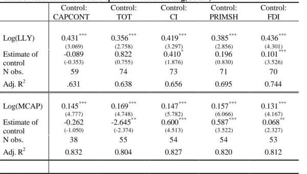
In section 2, the difference between domestically diversifiable risk and aggregate risk was discussed. Domestic insurance markets cannot diversify aggregate risk – access to international insurance markets is necessary for that purpose. In Table 3, we show the result of some tests for LLY and MCAP that consider these issues.16 In the first column we add the index of international financial openness. The sign of this variable is negative (although not significant) as we would expect it to be if access to international financial markets help facilitate an open trade policy. Including the variable CAPCONT does not affect the estimates of LLY and MCAP. Next, terms of trade shocks, TOT, are included which also has a limited effect on the estimates. In the next two columns, we control for variables likely to increase aggregate external risk. The first of these variables is an index on the product concentration of exports, CI,17 the second the share of primary exports of all exports, PRIMSH. It is reasonable to assume that a high value on either of these variables will increase aggregate income volatility caused by price movements on the international markets. Since domestic risk markets cannot diversify aggregate risk, controlling for external risk is the equivalent to controlling for non-diversifiable risk. The inclusion of these variables does not affect the results for LLY or MCAP. In the last column we include the share of foreign direct investments to GDP, FDI, in order to account for the possibility of a

16

The results are essentially the same for DC. The reason why both LLY and MCAP are presented is that the sample differs quite a bit between the variables.

17

The Gini-Hirschman index of concentration over 239 three-digit SITC export categories, calculated by UNCTAD.

spurious correlation between financial development and trade.18 It is plausible that FDI is positively related to both trade and financial development. This inclusion does not affect the basic results.

[Table 3 here]

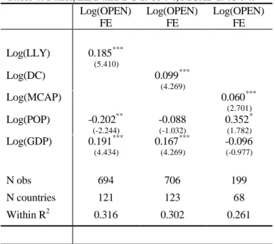
5.3 Openness: Panel results

By using a panel of data, we can go beyond the simple cross-section approach, controlling also for time and country specific effects, as well as bringing time into the analysis. The baseline panel specification is:

Openit = α + β1AREAi + β2POPit + β3DISTi + β4GDPit

+ β5FDit + β6Regioni + λt + vi + εit

Where λt is a time-specific effect, constant over countries, vi is a country-specific

effect, constant over time, and εit is the usual residual. AREA and DIST will not be

included in fixed effects estimations since these variables are time-invariant and can hence not be distinguished from the country specific effects. We introduce further variables later on.

The baseline panel results are presented in Table 4. The results are very similar to the ones in the cross-country setting, although the point estimates on our proxies for financial development are somewhat smaller. We have also run random effects regressions, but since these results are similar to the fixed effect estimations, we do not present them.19 More generally, the fixed effects approach is an attempt to account for the changes in openness which have occurred between 1960-94. To account for these changes, we should need more (time varying) explanatory variables than the ones we have included in the baseline regressions. However, the result that financial

18

We have also controlled for the investment share to GDP, human capital, and population density but this does not affect the results.

19

The great exception in the difference in explanatory power – the ‘within’ R2 that applies to fixed effect estimations and the ‘overall’ R2 applying to random effects. The overall R2 is between 0.7-0.8 depending on sample and specification. Since some of our control variables for trade are time invariant (DIST, AREA, regional dummies), it should be of no surprise that the within R2 is much lower than the overall R2.

development is positively related to openness, even after controlling for both fixed country effects and time-specific events, is encouraging for our basic hypothesis.

[Table 4 here]

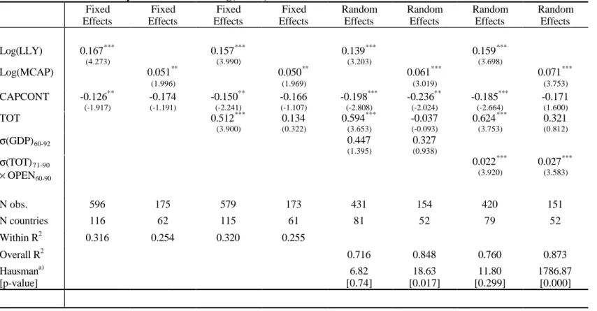
Aggregate risk, once again

To check the robustness of the panel results, especially with respect to aggregate and domestically non-diversifiable risk, we continue our study by including additional control variables. The results from these regressions are reported in Table 5.20 The first variable we include is CAPCONT, the index capital controls. As we would suspect the sign of the coefficient is negative, although the statistical significance varies between specifications. The negative sign gives support for the hypothesis that international risk sharing is an important determinant of trade policy. In section 2 we mentioned some caveats with this measure. Most importantly, capital controls can effectively work as trade restrictions, thus belonging on the left hand side of the regression. Regardless of the exact mechanism involved, however, the sign should be negative. Domestic financial markets still have a positive and significant impact on trade in all specifications. Hence we can conclude that the basic result is not due to a correlation between international financial restrictions and financial development. Both the development of domestic asset markets and the integration on international financial markets have independent effects on openness to trade.

[Table 5 about here]

Next, we include TOT, terms of trade shocks. TOT is defined as the growth rate of export prices minus the growth rate of import prices. We would expect the sign of this coefficient to be positive: A country is likely to trade more if export prices are rising and import prices are falling (or growing at a slower rate). This prediction is supported by the data and the inclusion of TOT does not affect the point estimates of LLY and MCAP (TOT is not included in the baseline specification since it is not available for the full time period).

20

All specifications have been estimated for DC as well. These regressions are virtually identical to the LLY-regressions so we do not present the results.

In the cross-section regressions we had to rely on export concentration, CI, and the share of primary resources in exports, PRIMSH, as proxies for aggregate external risk. The panel setting allows for more direct ways of approaching this problem. In columns 5 and 6 of Table 5, we control for total aggregate risk as measured by the standard deviation of per capita GDP during the period 1960-92. The variable is not significant and does not affect the coefficients on LLY or MCAP. In the last two columns, we control for aggregate external risk, measured by the standard deviation of terms of trade multiplied by average openness. Given its construction, it is of no surprise that this variable is positively related to openness. Since the key estimates are not affected by these inclusions, we conclude that the effect of financial markets on openness is not caused by a correlation with external risk. Rather, the stability of the coefficient even after the inclusion of aggregate risk measures indicates that domestic risk sharing is what matters for openness. As our controls for aggregate risk are time-invariant and hence we must use random effects estimations for the last four regressions.21 For these estimations, we perform the Hausman specification test. If the empirical model is correctly specified and the Hausman test returns a significant result, this can be interpreted as evidence that the individual specific effects and the regressors are correlated and hence that fixed effects estimation should be used. As can be seen in the last row of Table 5, the Hausman test indicates that the random effects estimator is appropriate for the LLY regressions, but not for the MCAP regressions. Despite this limitation, we conclude that domestic asset markets does have an independent positive relation with openness to trade, and that access to international asset seems to have a positive impact on trade, although this result is somewhat weaker.

5.4 Causality

So far, we have established a robust relationship between our proxies for financial development and openness to trade, but we have been silent on the issues of causality and the possibility of simultaneity. Recent studies suggest that greater openness to trade increases investment (see for example Wacziarg [1998]). Investments might in turn influence our measures of financial market development. Second, increased exposure to the fluctuations of the international market could increase the demand for

21

It should also be noted that the effect of aggregate risk, measured in these ways, is captured in the country specific fixed effects when running fixed effects estimations.

portfolio diversification. Finding a causal link from financial development to trade would lend specific support for the Feeney-Hillman [1998] hypothesis. The reverse causality, from trade to financial development, would not, however, contradict the underlying theoretical reasoning. Finally, although the Feeney and Hillman story suggests that causality runs from well-developed financial markets to trade policy, one can easily imagine political decisions affecting both variables simultaneously.

In order to explore the causality aspects, we first turn to the concept of Granger causality tests. The Granger test amounts to checking whether the lagged independent variables are jointly significant in a regression of the dependent variable on its own lagged values, i.e. a regression of the following kind:

The inclusion of the lagged dependent variable on the RHS creates a dynamic panel data problem: The lagged dependent variable is correlated with the fixed effect. To eliminate the bias caused by the presence of fixed effects, the equation is estimated in first differences. Since first the differentiation induces MA(1) residuals, the lagged difference of the dependent variable has to be instrumented for. This will be done using the twice-lagged difference and the twice-lagged level of the dependent variable as instruments.22

The estimates presented in Table 6 only include one lag, since 5-year averages make the time series rather short. Columns 1 and 2 show that the causality run both ways. LLY and DC do Granger cause openness, but there is also an effect of openness on the two proxies for financial development. MCAP, however, does not Granger cause OPEN instead the causality clearly runs in the opposite direction. Thus, which conclusion to draw depends on which proxy is used. Judging by the result for DC and LLY there is an effect of financial markets on trade, while MCAP shows that there is no such effect. It should be kept in mind that we have very few time-periods available when testing for causality using MCAP.

22

The dynamic panel data problem and its solutions are discussed in Baltagi [1995], chapter 8.

it i r it n r r r it n r r it

y

X

v

y

=

α

+

α

+

β

+

+

ε

∑

∑

[Table 6]

5.5 Simultaneity

In order to take into account the possible simultaneity indicated in section 5.4, we use instruments for financial development to see if the exogenous component of each of the proxies is significant. Finding instruments for financial development that are not correlated with trade policy is not an easy task. LaPorta et al. [1997] have come up with a number variables that could possibly serve our purposes, however. Unfortunately, these variables are all time-invariant, making panel regressions impossible.23 Instead we limit our focus to the 1990-94 cross-section and attempt to instrument for our three proxies of financial development. The instruments we use are; (i) an index of minority shareholder protection that takes a value between 0-6 with a higher value indicating stronger minority rights; (ii) a ‘rule of law’ index constructed by the risk rating agency International Country Risk (ICR) that assesses the law and order tradition of a country and ranges between 0-10, with lower scores for less tradition of law and order; (iii) the number of assassinations per million inhabitants. We use these instruments in order to capture the ideas that the protection of shareholders, an effective legal system, and a relatively safe environment are crucial elements for the development of financial markets. Why these instruments should have a relation to trade policy is less clear, and below we test for an independent effect of the instruments on openness to trade. Using these instruments limits the number of observations, and we end up with 36-38 countries in the regressions.Even though the sample is limited, we see in Table 7 that LLY, DC, and MCAP are all significant with the expected sign. The level of significance in a bit lower than in the OLS-estimations, but this should be of no surprise since we lose efficiency by using instrumental variables. Compared to the OLS-estimates in Table 2, all point estimates are much larger, suggesting elasticities between 0.2-0.6.24

[Table 7 here]

In order to account for the validity of the instruments, we also report the test statistics from the Hansen overidentification test in Table 7. This test assesses if the

23

As explained above, all time-invariant variables are captured in the country specific fixed effects.

24

instruments have an independent effect of openness to trade beyond their ability to explain cross-country variation in financial development. The test statistic is obtained by running the residuals from the second stage regression on the instruments and multiplying the R2 from this regression with the number of observations. Under the null-hypothesis that the instruments are not correlated with the error term, the test is distributed χ2 with (j-k) degrees of freedom, where j is the number of instruments, and k the number of variables instrumented for. Since the 10% critical value equals 4.61, all three IV-regressions pass the test by a wide margin.

Using the instrumental variables of financial development on the Sachs-Warner index does not yield any significant results. One reason could be that the instruments are from the late 1980’s or the early 1990’s, while the Sachs-Warner index is an average between 1950-1994. Thus, even if the results had been significant, we would have had reasons to question the exogeneity of the instruments.

These results are broadly consistent with the results on Granger causality. LLY and DC Granger cause OPEN, and have an exogenous effect on OPEN when using instrumental variables. MCAP seems to have an exogenous effect on openness, even though the Granger tests tell a different story.

Finally, we consider the possibility that both openness and financial development are simultaneously caused by the same underlying variable, not yet included in the regressions. One obvious possibility is that market friendly policies in general could affect both financial development and trade policies. To control for this, an index of “regulatory burden” described in Kaufmann et.al. [1999] is added to the regressions. This index is a combination of measures of market unfriendly practices. Further, dummy variables of a country’s legal origin as described in LaPorta et.al. [1997] are included on the right hand side of the regressions. The inclusion of these variables does not affect the results and the regressions are not presented.

6. Conclusion

Previous work on the relation between openness to trade and financial markets has been purely theoretical. This paper is a first attempt to empirically investigate if

financial markets have an impact on trade restrictions. Our major finding is that there does exist a strong, positive relationship between openness to trade and domestic financial development. In addition, the degree of integration on international financial markets has an independent, positive, effect on openness to trade.

This positive relation is shown to hold for two out of three proxies of financial development when the Sachs-Warner index is used as a measure of trade policy. Further, all three proxies enter positively into cross-section and panel estimations using (structurally adjusted) trade as a measure of openness. These results hold both in fixed and random effects-settings, even when controlling for a number of factors affecting trade. Some evidence of simultaneity between trade and financial development is found, and the direction of causality seems to be running both from financial development to trade, and in the opposite direction. Considering the possible simultaneity, we find support for an exogenous effect of financial markets on openness to trade.

This paper can be seen as a complement to the recent literature suggesting that risk reducing policies and trade policy is interdependent. In an oft-quoted paper, Rodrik [1998] presents theoretical and empirical arguments that countries more open to trade show greater fluctuations in income, and that the government sector is expanded in order to reduce these fluctuations. Since risk is aggregate in his model, private risk diversification within a country is not possible. Rodrik argues informally and shows empirically, however, that policies that reduce risk between groups within a country are also an important response to openness to trade. Agell [1999] follows the same line of thought when showing that open countries are more prone to provide insurance through labor market regulations such as minimum wage laws and unemployment insurance than closed ones. The common theme in these two papers is that risk-increasing policies can be optimally combined with policies reducing risk. Our paper makes the point that private risk diversification can facilitate risk-increasing policies. This point should apply to other areas than trade policy and is of interest when discussing, among other issues, the timing and political feasibility of policy reform.

Our results qualify some conclusions drawn in the recent literature. Both Agell [1999] and Rodrik [1997] warn that the current trend towards globalization of economic

activity leads to a greater exposure to risk, and thus greater demand for risk-reducing reforms, while simultaneously reducing the scope for government interventions especially through taxation and labor-market regulations. However, globalization also encompasses financial markets. If domestic asset markets and the integration of international asset markets facilitate liberal trade policies, as our results suggest, better domestic and international financial markets may well alleviate the negative effects of globalization pointed out by Agell and Rodrik.

Appendix Table A1: Descriptive statistics

Variable (years available)

Description Source Mean Standard deviation

N obs

Assassina-tions

Number of assassinations per million inhabitants World Bank1 0.261 0.474 70 AREA (1960-94)

Land area in km2 WDI 761052 1693138 134 CAPCONT

(1967-92)

Restrictions index on inter-national capital movements

IMF 0.503 0.301 757

CI (1990)

Export concentration index, defined in text UNCTAD 0.401 0.247 122 DC (1960-94) Financial resources to private sector, % of GDP IMF-IFS 30.809 26.148 797 DIST (1960-94)

Distance to 20 major trading economies

Barro-Lee 5.953 2.311 90 FDI

(1990-94)

Foreign direct investment, net inflow, % of GDP

WDI 1.798 2.997 126

Log(GDP) (1960-92)

(Log of) real per capita GDP PWT 7.685 1.027 853 LLY

(1960-94)

Liquid liabilities, % of GDP IMF-IFS 36.534 24.461 783 MCAP

(1987-94)

Value of listed companies, % of GDP World Bank1 26.975 40.976 217 Minority rights

Index of minority share holder protection World Bank1 2.441 1.231 41 OPEN (1960-94) Exports + imports, % of GDP WDI 63.960 37.196 811 POP (1960-94)

Thousands of inhabitants WDI 28941 101986 880 PRIMSH

(1990)

Share of primary exports in total exports

WDI 0.657 0.313 116

Regulatory burden

Index of market unfriendly practices

World Bank2

0.137 0.795 124 Rule of law ICR index of law and order

tradition World Bank1 7.072 2.618 41 Sachs-Warner (1950-94) Index of openness, Defined in text SW 0.331 0.339 122 TOT (1965-92) Growth of merchandise export prices minus growth of import prices

Wacziarg [1998]

-0.0067 0.066 803

PWT stands for Penn world tables 5.6; WDI for World Bank, World Development Indicators;World Bank1 for the Financial Structure and Economic Development Database; World Bank2 for the World Bank Governance Indicators described in Kaufmann et.al. [1999]; UNCTAD for Handbook of

International Trade and Development Statistics of UNCTAD; IFC for International Finance Corporation, Emerging Stock Market Factbook; IMF for the IMF’s Exchange arrangement and

Exchange Restrictions;IMF-IFS for IMF’s International Finance Statistics; Barro-Lee for Barro and Lee [1994]; SW for Sachs and Warner [1995]. PWT and Barro-Lee are available free of charge from http://www.nber.org. The Financial Structure and Economic Development Database and the

Table A2: Correlation between main variables of interest (1990-94 cross section)

OPEN AREA DIST POP SW LLY DC MCAP

GDP 0.164* (107) 0.190** (107) -0.516*** (80) -0.043 (109) 0.750*** (106) 0.577*** (104) 0.752*** (106) 0.394*** (69) OPEN -0.291*** (130) -0.038 (90) -0.209*** (130) 0.342*** (120) 0.459*** (125) 0.221*** (127) 0.504*** (76) AREA 0.099 (91) 0.542*** (136) 0.018 (122) 0.003 (128) 0.167** (130) 0.003 (76) DIST 0.104 (92) -0.409*** (91) -0.302*** (86) -0.297*** (88) -0.054 (61) POP -0.095 (124) 0.116 (128) 0.143* (130) -0.068 (76) Sachs-Warner 0.572*** (116) 0.641*** (118) 0.436*** (75) LLY 0.737*** (128) 0.512*** (73) DC 0.622*** (75)

*** Indicate significance at 1%-level, ** at 5%-level, * at 10%-level. Figures in parentheses are number of observations. Note that the above correlations are virtually the same for the full sample of observations.

References

Agell, J. [1999], “On the benefits from rigid labor markets: Norms, Market Failures, and Social Insurance”, Economic Journal, 109, F143-F164.

Alesina, A. and R. Wacziarg [1998], “Openness, Country Size and Government”, Journal of Public Economics, 69, 305-321.

Anderson, J. and P. Neary [1998], “Measuring the Restrictiveness of International Trade Policy”, mimeo, chapters 2-4.

Baltagi, B. [1995], Econometric Analysis of Panel Data, Wiley, Chichester. Barro, R. and J-W. Lee [1994], “Data Set for a Panel of 138 Countries”, mimeo Harvard University.

Cassing, J. [1980], “Alternatives to Protectionism”, in J. Levenson and J.W. Wheeler [eds.], Western Economies in Transition, Westview Press, Boulder.

, A. Hillman, N. Long [1986], “Risk Aversion, Terms of Trade Uncertainty and Social-Consensus Trade Policy”, Oxford Economic Papers, 38, 234-242.

Clark, T. and K. Shin [2000] “The Sources of Fluctuations Within and Across Countries” in Gregory D. Hess (ed.), Intranational Economics, forthcoming Cambridge University Press.

Corden, M. [1974], Trade Policy and Economic Welfare, Clarendon Press, Oxford. Dixit, A. [1987], “Trade and Insurance with Moral Hazard”, Journal of International Economics, 23, 201-220.

. [1989a], “Trade and Insurance with Adverse Selection”, Review of Economic Studies, 56, 235-248.

. [1989b], “Trade and Insurance with Imperfectly Observed Outcomes”, Quarterly Journal of Economics, 104, 195-203.

Eaton, J. & G. Grossman [1985], “Tariffs as Insurance: Optimal Commercial Policy when Domestic Markets are Incomplete”, Canadian Journal of Economics, 18, 258-272.

Feeney, J. & A. Hillman [1998], “Endogenous trade liberalization in the presence of domestic and international asset markets”, mimeo University of Michgan.

____ and ____ [2000] “Privatization and the Political Economy of Strategic Trade policy”, forthcoming International Economic Review.

Ghosh, A. and H. Wolf [1997] “Geographical and Sectoral Shocks in the U.S. Business Cycle”, NBER Working Paper #6180.

Gottschalk, P. and R. Moffit [1994] “The Growth of Earnings Instability on the US Labor Market”, Brookings Papers on Economic Activity 2, 217-254.

Harrison, A. [1996], “Openness and Growth: A Time-Series, Cross-Country Analysis for Developing Economies”, Journal of Development Economics, 419-447.

Hillman, A. [1977], “The Case for Terminal Protection for Declining Industries”, Southern Economic Journal, 44, 155-160.

Kaufmann, D., A. Kraay, and P. Zoido-Lobaton [1999] “Governance Matters”, World Bank Working Paper #2196.

King, R. & R. Levine [1993a]: “Finance and Growth: Schumpeter Might Be Right”, Quarterly Journal of Economics, 108, 717-737.

, and . [1993b]: “Finance, Entrepreneurship and Growth”, Journal of Monetary Economics, 32, 513-542.

Kraay, A., N. Loayza, L. Servén, J. Ventura [2000] “Country Portfolios”, mimeo World Bank.

LaPorta, R., F. Lopez-de-Silanes, A. Schleifer, R. Vishny [1997], “Legal Determinants of External Finance”, Journal of Finance, 52, 1131-1150. Lee, J-W. [1993], “International Trade, Distortions, and Long-Run Economic Growth”, IMF Staff papers, 40, 299-328.

Levine, R. and S. Zervos [1998], “Stock Markets, Banks, and Economic Growth”, American Economic Review, 88, 537-58.

Lewis, K. [1995] “Puzzles in International Financial Markets”. In Handbook of

International Economics vol.III, edited by G. Grossman and K. Rogoff. Amsterdam: North-Holland.

Lewis, K. [1996] “What Can Explain the Apparent Lack of International Consumption Risk Sharing?”, Journal of Political Economy, 104:2, 267-297. Newbery, D. and J. Stiglitz [1984], “Pareto Inferior Trade”, Review of Economic Studies, 51, 1-12.

Rodrik, D. [1997], “Trade, social insurance, and the limits to globalization.” NBER Working paper 5905.

. [1998], “Why do more open economies have bigger governments?”, Journal of Political Economy, 106, 997-1032.

Sachs, J. and A. Warner [1995], “Economic Reform and the Process of Global Integration”, Brookings Papers of Economic Activity, no. 1, 1-118.

Stulz, R. [1999] “Globalization of Equity Markets and the Cost of Capital”, NBER Working Paper #7021.

Tamirisa, N. [1999] “Exchange and Capital Controls as Barriers to Trade”, IMF Staff Papers, 46:1, 69-88.

Tesar, L. [1995] “Evaluating the Gains from International Risk-sharing”, Carnegie Rochester Conference Series on Public Policy, 42, 95-143.

Traca, D. [2000] “Globalization, Wage Volatility and the Welfare of Workers”, mimeo INSEAD.

Wacziarg, R. [1998], “Measuring the Dynamic Gains from Trade”, World Bank Policy Research Paper 2001.

Table 1A: Sachs-Warner index SW Average SW Average SW Average Constant -4.403 (-0.547) 18.290* (1.893) 7.767 (1.156) LLY 0.423*** (3.454) MCAP 0.111 (1.250) DC 0.382** (2.404) GDP 0.003** (2.168) 0.002 (0.241) 0.002 (1.540) AREA -0.800 (-0.602) 0.188 (0.160) -1.147 (0.413) POP -19.015 (-1.155) -38.133* (-1.990) -30.294 (-1.529) OECD 27.559*** (2.666) 32.323* (1.971) 24.081** (2.182) LAAM 14.920* (1.931) -4.433 (-0.415) 7.729 (1.001) SAFRICA 2.064 (0.274) -1.141 (-1.222) -5.517 (-0.745) EASIA 40.023*** (3.208) 45.611*** (3.146) 32.430** (2.538) N Countries 114 55 116 Adj. R2 0.552 0.639 0.552

*** Indicate significance at 1%-level, ** at 5%-level, * at 10%-level. t-statistics based on robust standard errors in parentheses.

Table 1B: Sachs-Warner index SW Average SW Average SW Average Constant 1.044 (0.133) 11.330 (0.625) 11.859* (1.708) LLY(1960) 0.374*** (3.401) MCAP(1975) 0.380* (1.976) DC(1960) 0.310 (1.562) GDP 0.002 (1.468) 0.003 (0.241) 0.002 (0.924) AREA -0.251 (-0.182) -0.556 (-0.526) 0.001 (0.001) POP -20.694 (-1.330) -21.471 (-0.721) -29.887* (-1.746) OECD 34.532*** (3.056) 35.631 (1.592) 38.831*** (3.435) LAAM 14.763* (1.943) -4.381 (-0.247) 8.892 (1.166) SAFRICA 0.353 (0.042) -24.373 (-1.213) -8.524 (-1.028) EASIA 51.316*** (3.608) 46.052** (2.276) 48.164*** (3.221) N Countries 87 35 87 Adj. R2 0.620 0.680 0.638

*** Indicate significance at 1%-level, ** at 5%-level, * at 10%-level. t-statistics based on robust standard errors in

Table 2: Baseline cross section 1990-94

Log(OPEN) Log(OPEN) Log(OPEN) Log(OPEN)

Log(LLY) 0.412*** (3.988) Log(DC) 0.197*** (2.789) Log(MCAP) 0.138*** (4.784) Log(AREA) -0.030 (-0.845) -0.017 (-0.551) -0.025 (-0.774) -0.017 (-0.709) Log(DIST) -0.289*** (-2.801) -0.343*** (-3.150) -0.335*** (-0.335) -0.486*** (-5.161) Log(POP) -0.223*** (-4.683) -0.208*** (-5.315) -0.223*** (-5.608) -0.252*** (-7.790) Log(GDP) 0.065 (0.759) -0.052 (-0.658) -0.052 (-0.593) -0.176** (-2.180) OECD -0.352** (-2.178) -0.265 (-1.558) -0.357** (-2.037) -0.273* (-1.650) LAAM -0.298** (-2.355) -0.010 (-0.064) -0.229** (-1.666) -0.205* (-1.677) SAFRICA -0.99 (0.560) 0.220 (1.289) 0.009 (0.055) 0.183 (1.170) EASIA 0.525*** (3.274) 0.610*** (3.737) 0.458*** (2.684) 0.533*** (4.079) Constant 6.602*** (7.252) 5.628*** (7.427) 6.851*** (9.127) 8.669*** (11.250) N obs. 77 75 77 55 Adj. R2 0.5518 0.635 0.592 0.793

*** Indicate significance at 1%-level, ** at 5%-level, * at 10%-level. t-statistics based on robust standard errors in parentheses.

Table 3: Additional controls. Dependent variable is Log(OPEN) Control: CAPCONT Control: TOT Control: CI Control: PRIMSH Control: FDI Log(LLY) 0.431*** (3.069) 0.356*** (2.758) 0.419*** (3.297) 0.385*** (2.856) 0.436*** (4.301) Estimate of control -0.089 (-0.353) 0.822 (0.755) 0.410* (1.876) 0.196 (0.830) 0.101*** (3.526) N obs. 59 74 73 71 70 Adj. R2 .631 0.638 0.656 0.695 0.744 Log(MCAP) 0.145*** (4.777) 0.169*** (4.748) 0.147*** (5.782) 0.157*** (6.066) 0.131*** (4.167) Estimate of control -0.262 (-1.050) -2.645** (-2.374) 0.600*** (4.513) 0.587*** (3.522) 0.068** (2.327) N obs. 38 55 54 54 53 Adj. R2 0.832 0.804 0.827 0.820 0.812

***Indicate significance at 1%-level, ** at 5%-level, * at 10%-level. t-statistics based on robust standard errors in parentheses. CAPCONT is an index of openness to international financial markets; TOT is the change in terms-of trade; CI is the export concentration index; PRIMSH is the share of primary resources in exports; FDI is foreign direct investments. All regressions include regional dummies, Log(AREA), Log(POP), Log(DIST), Log(GDP) and a constant.

Table 4: Panel, LLY and DC 1960-94, MCAP 1975-94. Log(OPEN) FE Log(OPEN) FE Log(OPEN) FE Log(LLY) 0.185*** (5.410) Log(DC) 0.099*** (4.269) Log(MCAP) 0.060*** (2.701) Log(POP) -0.202** (-2.244) -0.088 (-1.032) 0.352* (1.782) Log(GDP) 0.191*** (4.434) 0.167*** (4.269) -0.096 (-0.977) N obs 694 706 199 N countries 121 123 68 Within R2 0.316 0.302 0.261

*** Indicate significance at 1%-level, ** at 5%-level, * at 10%-level. t-statistics based on robust standard errors in parentheses. All regressions include time-period dummies and country-specific fixed effects that are jointly significant.

Table 5: Additional tests. Dependent variable is Log(OPEN) Fixed Effects Fixed Effects Fixed Effects Fixed Effects Random Effects Random Effects Random Effects Random Effects Log(LLY) 0.167*** (4.273) 0.157*** (3.990) 0.139*** (3.203) 0.159*** (3.698) Log(MCAP) 0.051** (1.996) 0.050** (1.969) 0.061*** (3.019) 0.071*** (3.753) CAPCONT -0.126** (-1.917) -0.174 (-1.191) -0.150** (-2.241) -0.166 (-1.107) -0.198*** (-2.808) -0.236** (-2.024) -0.185*** (-2.664) -0.171 (1.600) TOT 0.512*** (3.900) 0.134 (0.322) 0.594*** (3.653) -0.037 (-0.093) 0.624*** (3.753) 0.321 (0.812) σ(GDP)60-92 0.447 (1.395) 0.327 (0.938) σ(TOT)71-90 × OPEN60-90 0.022*** (3.920) 0.027*** (3.583) N obs. 596 175 579 173 431 154 420 151 N countries 116 62 115 61 81 52 79 52 Within R2 0.316 0.254 0.320 0.255 Overall R2 0.716 0.848 0.760 0.873 Hausmana) [p-value] 6.82 [0.74] 18.63 [0.017] 11.80 [0.299] 1786.87 [0.000]

*** Indicate significance at 1%-level, ** at 5%-level, * at 10%-level. t-statistics based on robust standard errors in parentheses. All regressions include Log(POP), Log(GDP) and time period dummies. The random effects estimates also include regional dummies, Log(AREA), and Log(DIST). σ(GDP)60-92 is the standard deviation of GDP 1960-92, σ(TOT)71-90 is the standard deviation of log differences in terms of trade

1971-90, OPEN60-90 is average openness 1960-90. a)

The Hausman test statistics is χ2 distributed with the same degrees of freedom as the number of explanatory variables. The p-value indicates at which probability we can reject the hypothesis that the fixed effects and the regressors are correlated.

Table 6: Granger causality between LLY/DC/MCAP and OPEN.

∆(OPEN) ∆(OPEN) ∆(OPEN)

∆(OPEN) t-1 0.289 (0.699) -0.082 (-0.222) 1.231 (0.363) ∆(LLY) t-1 0.277 ** (2.521) ∆(DC) t-1 0.148 ** (2.102) ∆(MCAP) t-1 -0.126 (-0.406) N obs 476 403 83 ∆(LLY) ∆(DC) ∆(MCAP) ∆(LLY) t-1 0.430 ** (2.233) ∆(DC) t-1 0.462 ** (2.193) ∆(MCAP) t-1 1.129 ** (2.119) ∆(OPEN) t-1 0.115 *** (2.646) 0.212*** (3.427) 1.565*** (2.935) N obs. 390 3.427 34

***Indicate significance at 1%-level, ** at 5%-level, * at 10%-level.t-statistics based on robust standard errors in parentheses. The lagged difference of the dependent variable is instrumented using the twice-lagged difference and the twice-lagged level of the dependent variable.

Table 7: Instrumental variables 1990-94

Log(OPEN) Log(OPEN) Log(OPEN)

Log(LLY) 0.606** (1.993) Log(DC) 0.606** (2.011) Log(MCAP) 0.276* (1.866) N obs. 36 38 37 R2 of residuals on instruments 0.004 0.0001 0.053 OIR-testa) 0.144 0.004 1.961

*** Indicate significance at 1%-level, ** at 5%-level, * at 10%-level. t-statistics based on robust standard errors in parentheses. Regressions include constant, Log(GDP), Log(AREA), Log(DIST), Log(POP), and regional dummies. Instruments are an index of minority shareholder rights, the ‘rule of law’ index by ICR, and the number of assassinations per million inhabitants. a) The null hypothesis of the overidentification test is that the instruments are not correlated with the residuals from the second stage regression. Critical values for the test (2 d.f.): 10%=4.61, 5%=5.99.