METHODOLOGY
Guy R. West
Department of Economics The University of Queensland
ABSTRACT
The methodology in many studies involving input-output analysis appears to be often misunderstood, particularly in the way multipliers are used. The preoccupation with multipliers has led in many cases to incorrect analytical procedures; for example, there is a temptation to first derive a multiplier and then use this multiplier to calculate the total impact on the economy. This paper demonstrates that this approach is often erroneous and can result in significant errors. In addition, the importance of determining how imports are treated when using input-output in empirical situations is discussed. This is particularly relevant when using input-output tables in developing countries. Other issues which are clarified include the use of output multipliers, state versus regional multipliers and impacts, expenditure switching and table balancing.
METHODOLOGY
1. INTRODUCTION
In spite of the well-known theoretical limitations of input-output analysis, there appears to be no abatement in the number of economic impact studies being performed in the input-output framework. This is particularly true at the regional (sub-state) level, and is understandable given the lack of more sophisticated modelling systems available at this level. If anything, the use of input-output at the regional level seems to be increasing. Yet, in spite of its well documented theoretical structure, there is a wide spread lack of consistency in how the model is used; in fact, many applications appear to be based on incorrect analytical procedures.
This paper attempts to clarify what appears to be some common misconceptions in the application of input-output analysis. Firstly, the distinction is drawn between the conventional input-output multipliers and the impact multipliers derived from an impact study. Rather than use the multipliers to calculate the total impacts, the reverse is generally true; impact multipliers should be calculated from the total impacts. A note of warning is also given with respect to the closed model. The importance of determining how imports are treated when using input-output in empirical situations is discussed. Finally, a brief discussion of the limitations of the standard input-output model is presented, which lays the foundation for the search for more sophisticated models which, hopefully, are more ‘realistic’ in empirical applications.
2. INPUT-OUTPUT MULTIPLIERS
One of the first questions most often asked of consultants undertaking an economic impact exercise is: "What is the multiplier?". There appears to be a general confusion, even by analysts working in the input-output field, as to the use of multipliers in impact studies. First of all, the important thing to consider in an impact study is not the size of the multiplier but the magnitude of the total impact on output, value added, income and employment. A small multiplier can correspond to a large total impact and a large multiplier to a small impact on the economy depending on the size of the initial change in final demand. Although multiplier values are a useful indicator, bearing in mind they only show relativities and in some cases don't even express cause and effect relationships, they are not the main reason for the undertaking the impact analysis.
Secondly, generally speaking, the conventional input-output multipliers are not used to calculate total impacts. Rather, it is the other way around; an "impact" multiplier can be constructed only
Consider a simple n = 2 sector regional economy. The transactions flows can be represented by the system of equations thus:
(1) X = F + X + X X = F + X + X 2 2 22 21 1 1 12 11
where Xij = output of local sector i purchased by sector j, Fi = total final demand or sector i's output, and
Xi = total output (production) of sector i.
By dividing the transactions flows by their respective total output levels , the equations can be expressed in direct regional coefficient form:
Xij Xj (2) X = F + X a + X a X = F + X a + X a 2 2 2 22 1 21 1 1 2 12 1 11 or (3) X X = F F + X X a a a a 2 1 2 1 2 1 22 21 12 11
where a are the direct regional input or regional purchase coefficients. Here a is the amount purchased by sector j from sector i per unit of output of sector j. Equation (3) can be rearranged to give: X / X = ij j ij ij (4) F F = X X ) a -(1 a -a -) a -(1 2 1 2 1 22 21 12 11 or simply (4a) F = X ) A I (
where is the matrix of direct input coefficients, X is the vector of industry total outputs, and F is the vector of industry total final demands. This is the usual input-output relationship seen in the literature.
] a [ = A ij
The input-output (output) multiplier for sector j "is defined as the total value of production in all sectors of the economy that is necessary in order to satisfy a dollar's worth of final demand for sector j's output" (Miller and Blair, p.102). The output multiplier for sector 1, for example, would be calculated from equation (4) by setting the final demand for sector 1's output to unity and the remaining final demands to zero:
-1 (5) 0 1 ) a -(1 a -a -) a -(1 = X X 22 21 12 11 2 1
and summing X1 and X2.
Because of the linearity property of the model1, this can be extrapolated to other values of final demand for that sector's output. Thus, for example, a $10 increase in final demand of sector 1 would result in a total increase in production in all sectors of 10 times the value of
from equation (5). X + X1 2
Obviously, this example does not reflect the usual impact scenario; it would be unusual to experience an increase in only one sector's final demand. A more common scenario is that there are multiple changes in final demand or, conversely, no change in final demand if the impact of an existing industry, operating at current production levels, is of interest. In the former case, one can simply use equation (4), or if they were more enigmatic, sum the products of the multipliers times the change in final demand over all sectors. Yet a common practice is to insert the new expenditure into the intermediate quadrant as a new sector, calculate its multiplier, and multiply the multiplier value by the total expenditure level in order to measure the total impact of that expenditure on the economy. This is not correct, as is demonstrated in the following section.
3. IMPACT ANALYSIS
Impact analysis in an input-output framework is undertaken by manipulating the basic equation (4). The three most common scenarios confronting the analyst are: (a) the expansion of existing industries, (b) a new industry in the region, and (c) the economic significance of an existing industry. Each is considered in turn.
3.1 Existing Sectors Supply Additional Sales to Final Demand
In this scenario, the existing industries in the region increase their output in order to meet additional sales to final demand. This is the simplest, and probably most common, approach to impact analysis. The initial stimulus can be in any category of final demand; for example final 1 The properties of the input-output model are discussed later in this paper.
-1 *
-1
government expenditure, capital expenditure or exports. The impact on the economy is then the increase in production levels over all sectors required to meet the additional final demand. The input-output multiplier is obviously a special case of this scenario.
Suppose the additional final demands are and ∆ . The new industry production levels after the impacts are obtained from equation (4):
F1 ∆ F2 (6) ∆ ∆ F + F F + F ) a -(1 a -a -) a -(1 = X X 2 2 1 1 22 21 12 11 * 2 1
which, alternatively, can be rewritten to give the change in industry production levels in response to the additional final demands:
(7) ∆ ∆ ∆ ∆ F F ) a -(1 a -a -) a -(1 = X X 2 1 22 21 12 11 2 1
The sum of all the changes in industry production levels represents the impact on the economy resulting from the expansion in the levels of final demand. While the concept of a multiplier still applies, it is now defined as the ratio of the total change in production to the initial change in exogenous final demand, namely . This is commonly referred to as an impact multiplier in order to distinguish it from the more common input-output multiplier. The impact multiplier is in fact a weighted average of the input-output multipliers over all sectors, the weights being the .
) F + F ( / ) X + X (∆ 1 ∆ 2 ∆ 1 ∆ 2 Fi ∆
An alternative which is sometimes suggested is to treat the change in final demand as a new industry (column) in the intermediate quadrant. Provided the new row is null, we can then calculate the input-output multiplier for this sector in the manner described in the previous section. However, this will not be quite the same as the impact multiplier. It can be easily shown, through the properties of matrix partitioning, that the resultant input-output multiplier would be . The unit in the formula is the additional (over and above the original final demand change, ) "dollar's worth of final demand" for the new sector's output. In other words, this approach adds an additional unit change in final demand
which doesn't actually occur. ) F + F ( / ) X + X ( + 1 ∆ 1 ∆ 2 ∆ 1 ∆ 2 ∆F1 + ∆F2
2 Multiplying this multiplier value by the output level of the new
2
If the disaggregated multiplier is calculated, it shows the additional unit accrues to the newly created sector. However, in reality, there is no new sector.
sector would therefore overestimate the impact on the economy by the amount of the original final demand change3.
3.2 A New Industry Enters the Region
The second scenario reflects the situation of a new (and different) industry entering the region. The new industry is incorporated as an additional sector in the model, in the form of a new row and column in the transactions and direct coefficients matrix, representing the intermediate sales and purchases of the new industry. Subsequently, there may be changes in the direct coefficients as a result of increased production levels and substitution effects4.
The impact on the economy is the difference between the before and after production levels of all the sectors in the economy. Once the new industry is incorporated into the table, it can be treated as an existing sector and its economic significance can be measured. The recommended method for doing this is explained in the next section.
3.3 The Economic Significance of an Existing Industry
There are a number of ways of measuring the economic impact of an existing industry. One is to assume that the industry in question shuts down completely and to calculate the change in industry production levels before and after the shutdown. A second method is to calculate the impact resulting from the loss of all final demand sales by the industry in question. Both are discussed in turn.
Complete Shutdown of the Industry
3 If the new row contains some non-zero elements, the relationship is even more complicated and the
overestimation will be greater still.
4
Note this entails some readjustment of the original transactions, although not necessarily those in the intermediate quadrant, to ensure the new table is balanced (see Section 7 below).
To measure the economic impact of an existing industry producing at its current production level involves comparing the industry production levels both with and without the industry in question.5
Under this assumption, the remaining industries lose all purchases from and sales to the industry in question. Suppose the economy contains three sectors, as shown in equation (8),
(1-a11) -a12 -a13 X10 F10 (1-a ) -a 0 X F1 1 1 1 12 11 (8) F F = X X ) a -(1 a -a -a -) a -(1 a -0 3 0 2 0 3 0 2 33 32 31 23 22 21
and that we wish to estimate the impact of sector 3 on the economy. Remove the effect of sector 3 from the economy by making the third row and column of the input-output table null:
(9) 0 F = X X 1 0 0 0 ) a -(1 a - 1 2 1 3 1 2 22 21 5
In the previous scenario of a new industry entering the region, the industry had to be added to the table to get the 'with' case and the ‘without’ case is the status quo; in this scenario the industry has to be removed to get the 'without' case and the ‘with’ case is the status quo.
∆ ∆ (1-a ) -a 0 X F +a X0 3 13 1 1 12 11
Note that the 0 and 1 superscripts refer to the 'with' and 'without' output levels and final demands respectively. This procedure is based on the premise that the removal of the industry in question does not effect the purchasing patterns of the remaining industries. In other words, the remaining industries would still purchase the same amounts per unit of output from the other intermediate industries, but that purchases from sector 3 are replaced by imports. Thus, the goods and services produced by the industry in question do not have close substitutes in the remaining industries. This is in line with one of the basic assumptions of the input-output model, namely that the commodities produced by each industry are homogeneous products.6 Subtracting (9) from (8) gives: (10) ∆ ∆ ∆ F +a X +a X +a X X a + F = X X 1 0 0 0 ) a -(1 a -0 3 33 0 2 32 0 1 31 0 3 0 3 23 2 3 2 22 21
Noting that the last element of the vector on the right hand side is simply the base level total output from sector 3 (from equation (2)), and assuming that the final demands of sectors 1 and 2 remain unchanged, this can be rewritten as:
∆X (1-a ) -a 0 a X0 3 13 12 11 -1 1 (11) ∆ ∆ X X a 1 0 0 0 ) a -(1 a -= X X 0 3 0 3 23 22 21 3 2
The total impact of the industry of interest on the economy is ∆ which, in this
example, is equal to . The impact multiplier is now
. X + X + X1 ∆ 2 ∆ 3 X + X + X1 ∆ 2 03 ∆ X / ) X + X + X ( 0 3 3 2 1 ∆ ∆ ∆ 6
If we can estimate what the changes would be to the remaining industries after the sector of interest is removed, then these can be incorporated into equation (9).
Note that this is equivalent to deleting the row and column of the sector of interest and performing a final demand change impact analysis on the remaining (n-1) sectors with the new final demands equal to the removed industry's column transactions. The removed industry's production level is then added as part of the total impact on the economy.
In summary, to calculate the total impact on the economy, we make the row and column of the A matrix corresponding to the sector of interest all zeros. We then perform a standard final demand impact analysis with the final demand being the column of transactions of the sector of interest in the flow matrix, and with the final demand element corresponding to the sector of interest replaced by the initial production level of that industry.
As mentioned, the practice of calculating impacts using the conventional input-output multipliers will over-estimate the correct impacts depending on the level of intermediate sales by the industry in question. It is interesting to get an idea of the extent of the over-estimation, and Table 1 compares the impacts from the two methods for the 1986-87 28-sector Australian input-output table (Table 11, ABS, 1990). It can be seen that the total impacts derived from the input-output multiplier approach over-estimates the impact approach by as much as 32 percent in sector 14 (Basic metals and products), with five sectors having over 20 percent difference and sixteen sectors with over 10 percent difference. The only sector experiencing no difference between the two approaches is sector 25 (Ownership of dwellings), due to its having a null row in the intermediate quadrant. The results in Table 1 refer to the open model; if the closed model were used, the differences would be larger due to the relatively large elements in the household column.
This overestimation is understandable when we remember that the input-output multiplier assumes an expansion in final demand sales. However, when measuring the impact of an existing industry producing at its current production level, there is no expansion in final demand.
Table 1 Comparison of Industry Impacts, Open Model, Australia, 1986-87
Multiplier Method Shutdown Method Final Demand Method
Sector Output ($M) Rank Input-Output Multiplier Output ($M) Rank Impact Multiplier Percent Difference Output ($M) Rank 1 28,510.8 (11) 1.690 25,784.7 (10) 1.528 10.57 11,529.4 (13) 2 3,136.4 (28) 1.795 3,000.2 (28) 1.717 4.54 1,544.9 (27) 3 29,079.5 (10) 1.532 26,419.0 (9) 1.392 10.11 15,475.3 (10) 4 25,490.8 (13) 2.392 23,012.5 (12) 2.159 10.77 19,649.1 (8)
5 23,656.9 (14) 2.188 20,129.9 (14) 1.862 17.52 16,479.2 (9) 6 8,666.9 (25) 2.103 8,265.0 (25) 2.005 4.86 7,759.8 (16) 7 8,582.8 (26) 2.053 6,958.2 (27) 1.664 23.35 3,844.4 (24) 8 8,328.5 (27) 1.876 7,447.1 (26) 1.677 11.84 6,816.1 (18) 9 11,455.1 (22) 1.962 9,591.9 (22) 1.643 19.42 4,548.9 (21) 10 16,941.5 (20) 1.689 14,294.8 (19) 1.425 18.52 2,695.8 (25) 11 17,113.7 (19) 1.946 13,924.2 (20) 1.583 22.91 4,051.4 (23) 12 20,638.1 (15) 2.009 18,886.1 (15) 1.838 9.28 7,076.0 (17) 13 9,844.8 (23) 1.986 8,595.5 (24) 1.734 14.53 322.2 (28) 14 30,649.4 (8) 2.202 23,092.0 (11) 1.659 32.73 9,913.2 (15) 15 18,337.2 (18) 2.139 16,638.0 (17) 1.941 10.21 4,370.0 (22) 16 19,903.8 (17) 1.859 16,446.2 (18) 1.536 21.02 11,815.6 (12) 17 20,439.5 (16) 1.847 18,713.8 (16) 1.700 9.22 11,074.5 (14) 18 11,587.8 (21) 1.967 10,380.9 (21) 1.762 11.63 2,575.6 (26) 19 27,889.6 (12) 1.708 22,130.1 (13) 1.335 26.03 6,227.1 (19) 20 74,329.1 (2) 1.856 74,084.7 (2) 1.850 0.33 68,935.2 (1) 21 78,860.3 (1) 1.564 75,537.2 (1) 1.498 4.40 52,194.7 (3) 22 9,423.3 (24) 1.483 9,380.6 (23) 1.476 0.46 4,795.2 (20) 23 52,202.3 (5) 1.551 48,063.4 (5) 1.428 8.61 25,444.3 (7) 24 66,935.9 (3) 1.558 55,886.0 (4) 1.301 19.77 14,272.0 (11) 25 38,550.7 (6) 1.395 38,550.7 (6) 1.395 0.00 38,550.7 (4) 26 30,087.3 (9) 1.587 29,894.4 (8) 1.577 0.65 27,079.4 (5) 27 56,540.7 (4) 1.345 56,075.8 (3) 1.334 0.83 53,972.9 (2) 28 32,596.5 (7) 1.731 30,660.0 (7) 1.628 6.32 26,019.9 (6)
Loss of Final Demand Sales by the Industry
Another measure which is sometimes used as an indicator of the economic significance of an industry is to measure the impact on industry production levels resulting from the loss of all final demand sales by the industry in question. This approach arises directly from the basic assumption of the input-output model that output is demand generated through final demand sales.
The calculation procedure is quite straight forward, and simply involves multiplying the conventional input-output multiplier for the industry in question by the level of aggregate final demand of that industry. The reason this approach is sometimes suggested arises, as mentioned above, from the structure of the input-output model. If these calculations are applied to all the
sectors in the table, and the results summed, they will completely exhaust total intermediate output. However, one needs to be careful that the conclusions reached from the application to any individual industry are in line with expectations. For example, a large industry with most of its sales going to other local firms, with little or no sales to final demand which can occur, e.g., with some manufacturing or processing type industries where total production is absorbed by other local industries for further processing, would produce a measure of economic significance that would be very small or zero. On the other hand, if the industry does not sell much of its output to local firms, but exports most of its output in an unprocessed state, its measure of economic significance will be large.
The industry impacts for the Australian table are also provided in Table 1. It can be seen that the sector rankings differ depending on the procedure used. In the case of the final demand method, the impacts range from a high of $68,935.2 million for sector 20 (Construction) to a low of $322.2 million for sector 13 (Non-metallic mineral products). In the shutdown method, sector 2 (Forestry and fishing) has the smallest impact.
Although the example used above has been cast in terms of output levels, the significance indicators can just as easily be presented in terms of other variables, such as value added or employment. The choice of which measure described above is used will depend on the industry in question. In general, the measure most often used is complete shutdown. It must be remembered, however, that no measure can be regarded as completely realistic in a real world situation. They are only indicative measures which provide some indication of the economic significance of an industry on the local economy.
3.4 Mixed Variable Impacts
The three methods of impact analysis describe above, namely multipliers, changes in final demand and economic significance of a particular industry, can all be classified as special cases of the mixed variable approach to modelling impacts in an input-output framework. The only requirement necessary to uniquely solve the input-output equations in (4) is that each equation must have one predetermined variable, i.e. either Xj or .Fj 7
For example, suppose that the economy contains 3 sectors. From the basic equation (4), we have:
7 Actually, there is no reason why both
X and can't be predetermined. In this case, a necessary condition for solution is that the total number of predetermined variables from all equations must equal the total number of equations in the system.
(1-a11) -a12 -a13 X1 F1 X (1-a11) -a12 0 F1+a13X3 -1 1 (12) F F = X X ) a -(1 a -a -a -) a -(1 a -3 2 3 2 33 32 31 23 22 21
Now let the gross output of sector 3 be fixed as well as the final demands of sectors 1 and 2 . That is, the values of , F and are predetermined. Rearranging equation (12) by putting the predetermined variables on the right-hand side gives:
F1 2 X3 (13) (1-a )X X a + F 1 a a 0 ) a -(1 a -= F X 3 33 3 23 2 32 31 22 21 3 2 X1
which can be solved to find the values of the endogenous variables , and . Obviously, any combination of endogenous/exogenous variables can be used, and this approach provides a powerful tool for assessing a wide range of impact situations.
X2 F3
4. OUTPUT AND VALUE ADDED MULTIPLIERS AND IMPACTS
Output multipliers and the output effects in impact analyses refer to gross expenditure or turnover. Gross output measures are susceptible to multiple counting, because they sum all the intermediate transactions over all stages of production during the production process.8 Consequently, they substantially overstate economic activity. Therefore while output effects provide a measure of the increase in gross sales throughout the economy following an economic stimulus, they are inappropriate as a measure of the contribution to economic activity.
The preferred measure of net impact is value added, which is defined as wages and salaries and supplements paid to labour plus gross operating surplus plus indirect taxes less subsidies. The sum of all industry value added is equal to Gross Regional Product (GRP) - or Gross State Product (GSP) at the state level or Gross Domestic Product (GDP) at the national level - so value 8
See Burns and Mules, pp. 13-14 in Burns, Hatch and Mules (1986) or p. 7 of GSO (1995) for a simple example which clearly demonstrates this fact.
added impacts refer to the contribution to GRP. This is the preferred and consistent measure of economic activity. Output effects should only be used in exceptional circumstances.
5. REGIONAL AND STATE MULTIPLIERS
It is common practice in impact analyses to calculate impacts or multipliers at both regional and state (and perhaps national) levels. If both regional and state input-output tables are available, this would seem to be a simple process. One simply has to insert, e.g., the changes in final demand into the respective regional and state tables.
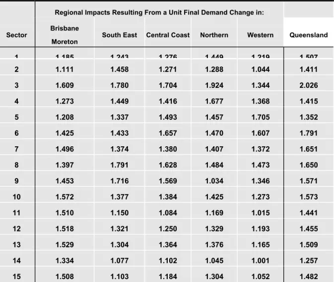
Suppose, for example, there is a stimulus of $1 to the final demand of sector 1 (Primary industry) in the Brisbane Moreton region of Queensland.9 Table 2, which gives the regional multipliers for five regions of Queensland, shows that the impact on the Brisbane Moreton region is $1.185. To measure the impact of the same $1 increase on Queensland, the usual reaction seems to be to insert the $1 stimulus into the final demand of sector 1 of the Queensland table. This results in an impact on the total Queensland economy of $1.507, as shown in the last column of Table 2.
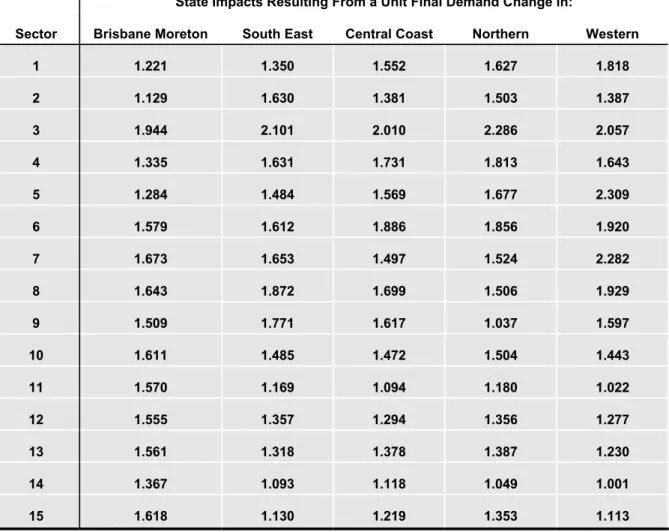
A little thought reveals that this practice for calculating the impacts at the state (or national) level is incorrect and can produce very misleading results. The reason is that the $1 stimulus to the final demand of sector 1 in the Queensland table is not the same $1 increase in just the Primary sector in the Brisbane Moreton region, but a $1 increase spread over all Primary sectors in the state, including the Brisbane Moreton, South East, Central Coast, Northern and Western regions. The $1.507 calculated from the Queensland table is actually a weighted average of the impacts on Queensland which would have occurred if each and every region incurred a $1 stimulus to its final demand. For example, the actual impact on Queensland resulting to a $1 change in the final demand of sector 1 in Brisbane Moreton is $1.221 (first column of Table 3), not $1.507.
9
The discussion in this section applies equally to multiple changes in final demand or other approaches to impact analyses. A unit change (i.e. multiplier) is used here for simplicity.
It can be shown that the state multipliers from a unit change in regional final demand will be higher than the state multiplier from a unit change in state final demand in regions which have a comparative advantage or are dominated by that particular activity, and less in those regions
which do not have a comparative advantage. This is clearly seen in Table 3, which gives the state multipliers resulting from unit final demand changes in each of five regions of Queensland and the corresponding Queensland multiplier for 1985-86. It can be seen that sector 1 (Primary industry) has larger multipliers from unit final demand changes in Central Coast, Northern and West Queensland, and smaller in Brisbane Moreton and South East, than for the state as a whole. Similarly, Sector 14 (Public administration) has a larger multiplier in Brisbane Moreton and smaller multipliers in South East, Central Coast, Northern and Western regions.
Table 2 Regional Output Multipliers, Open Model, Queensland, 1985-86
Regional Impacts Resulting From a Unit Final Demand Change in:
Sector Brisbane
Moreton South East Central Coast Northern Western Queensland
1 1 185 1 243 1 276 1 449 1 219 1 507 2 1.111 1.458 1.271 1.288 1.044 1.411 3 1.609 1.780 1.704 1.924 1.344 2.026 4 1.273 1.449 1.416 1.677 1.368 1.415 5 1.208 1.337 1.493 1.457 1.705 1.352 6 1.425 1.433 1.657 1.470 1.607 1.791 7 1.496 1.374 1.380 1.407 1.372 1.651 8 1.397 1.791 1.628 1.484 1.473 1.650 9 1.453 1.716 1.569 1.034 1.346 1.571 10 1.572 1.377 1.384 1.425 1.273 1.573 11 1.510 1.150 1.084 1.169 1.015 1.441 12 1.518 1.321 1.250 1.329 1.193 1.455 13 1.529 1.304 1.364 1.376 1.165 1.509 14 1.334 1.077 1.102 1.045 1.001 1.257 15 1.508 1.103 1.184 1.304 1.052 1.482
The correct method of calculating the impacts on regional industries at the state level involves the use of an interregional table. Single region state tables do not provide realistic measures of impacts incurred at the regional level on the state economy. The absence of an interregional state table does not justify the use of a single region state table as the results in Table 3 show. If this is
done, in studies involving the measurement of impacts on both the regional and state economies, the relationship between the regional impacts and the state impacts can be extremely misleading, if not absurd. For example, a $1 stimulus to Public Administration (sector 14) in Brisbane-Moreton results in an impact of $1.334 in Brisbane-Brisbane-Moreton (first column of Table 2). Applying the same $1 stimulus to the Queensland table gives a total state impact of $1.257 (last column of Table 2), which is less than the impact in Moreton. In fact, the $1 stimulus in Brisbane-Moreton gives a state impact of $1.367 (first column of Table 3).
Table 3 State Output Multipliers, Open Model, Queensland, 1985-86
State Impacts Resulting From a Unit Final Demand Change in:
Sector Brisbane Moreton South East Central Coast Northern Western
1 1.221 1.350 1.552 1.627 1.818 2 1.129 1.630 1.381 1.503 1.387 3 1.944 2.101 2.010 2.286 2.057 4 1.335 1.631 1.731 1.813 1.643 5 1.284 1.484 1.569 1.677 2.309 6 1.579 1.612 1.886 1.856 1.920 7 1.673 1.653 1.497 1.524 2.282 8 1.643 1.872 1.699 1.506 1.929 9 1.509 1.771 1.617 1.037 1.597 10 1.611 1.485 1.472 1.504 1.443 11 1.570 1.169 1.094 1.180 1.022 12 1.555 1.357 1.294 1.356 1.277 13 1.561 1.318 1.378 1.387 1.230 14 1.367 1.093 1.118 1.049 1.001 15 1.618 1.130 1.219 1.353 1.113 6. EXPENDITURE SWITCHING
When measuring the impact of a special event activity, such as a sporting event, trade exposition, etc., it is important not to simply take the direct expenditure of all visitors as being attributed to the activity. Local residents who visit the special event still contribute to the local economy. If
the event was not staged, they would spend their money on something else. Thus one has to be careful how this 'switching' of expenditure is handled, and in particular the relevant assumptions about what expenditure is included in the impact analysis.
It is often claimed that substitution effects between alternative expenditure in the region have no net effects on the economy. For example, according to the GSO (1995) guidelines (p.10):
Some expenditures simply represent a substitution effect where demand for one industry's output is switched to another, therefore providing little or no net stimulus to the state's economy. On this basis, expenditure of Queensland residents who attend special events in Queensland should be excluded from impact analyses.
While the general thrust of this argument is valid, it should not be accepted in all cases as a fait accompli. The assumption of switching of expenditures from one activity to another in the region having no net effect on the economy is an assumption of the economic base model, and is one of the reasons why input-output is preferred to economic base models. Whether there is a net gain, loss or no change after switching of expenditures occurs depends on the relative interconnectedness of the sectors involved. If the sectors which receive the additional expenditures are more interconnected or less import dependent than the sectors from which the expenditures were switched, there will be a net gain to the economy. Conversely, there would be a net loss if the sectors receiving the additional expenditures are less interconnected.
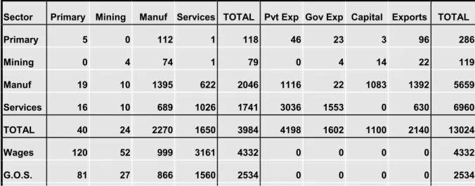
For a simple example which demonstrates this fact, consider the following 4-sector hypothetical transactions table:
Table 4 Hypothetical 4-Sector Transactions Table ($M)
Sector Primary Mining Manuf Services TOTAL Pvt Exp Gov Exp Capital Exports TOTAL
Primary 5 0 112 1 118 46 23 3 96 286 Mining 0 4 74 1 79 0 4 14 22 119 Manuf 19 10 1395 622 2046 1116 22 1083 1392 5659 Services 16 10 689 1026 1741 3036 1553 0 630 6960 TOTAL 40 24 2270 1650 3984 4198 1602 1100 2140 13024 Wages 120 52 999 3161 4332 0 0 0 0 4332 G.O.S. 81 27 866 1560 2534 0 0 0 0 2534
Ind Tax 10 2 58 101 171 469 0 5 3 648
Imports 35 14 1466 488 2003 987 7 152 15 3164
TOTAL 286 119 5659 6960 13024 5654 1609 1257 2158 23702
Employ 12717 3057 106616 306482 428872 0 0 0 0 428872
Suppose that there is a switch in demand expenditure from Primary to Manufacturing amounting to $2.1 million. The accepted method for estimating the resulting changes in output is from the equation (7) where ∆ 0 2.1 + 0 = F -2.1
The results are summarised in Table 5. Even though the initial change in final demand expenditure is zero, there is a net positive output flow-on effect in the economy, due to the more interrelated structure of the Manufacturing sector. However there is also a net decrease in value added, income and employment impacts. Agriculture contributes relatively more to Gross Regional Product per unit of output than Manufacturing, and similarly for employment and income since Agriculture is more labour intensive. Each million dollars of output produced by the Primary sector requires on average 44.46 workers, whereas only 18.84 employees are required (on average) to produce $1 million of Manufacturing output. Thus any cut-back in Primary production will (on average) have a greater impact on employment (and income) levels than a corresponding change in Manufacturing production.
Table 5 The Impacts Resulting from Switching Demand Expenditure from Primary to Manufacturing.
Output
($M) Value Added ($M) Income ($M) Employment (Persons)
Initial Change 0.00 -0.84 -0.51 -53.81
Flow-on
Effect 0.35 0.11 0.05 5.46
Total Impact 0.35 -0.72 -0.46 -48.35
Primary -2.09 -1.54 -0.88 -92.99
Mining 0.03 0.02 0.01 0.86
Manufacturing 2.48 0.84 0.44 46.71
Services -0.07 -0.05 -0.03 -2.94
0.35 -0.72 -0.46 -48.35
7. OPEN AND CLOSED MODELS AND TABLE BALANCING
A point which is often overlooked by analysts is the balancing of the household sector. When only the productive industries of the economy are regarded as endogenous, with household activity assumed exogenous, the model is referred to as being "open". These days, it is common practice to "close" the model with respect to households, on the assumption that the level of local production is a determinant in the level of household income, which in turn is largely spent locally and therefore influences the demand for local goods and services.
Irrespective of the arguments for or against full or partial closure, depending on the propensity to spend locally, the input-output model dictates that all corresponding endogenous row and column totals must be equal10. In many published tables, this restriction is not satisfied since the household row typically only includes wages and salaries and not other forms of income, and therefore the income row total is generally less than the consumption column total. In such cases, technically the results of impact analyses are invalid. In practice, this point is usually ignored, but one needs to be careful that the results are not distorted, particularly if changes in the final demand of the household sector, which is becoming more common, are considered as part of the impacting process.
8. ALLOCATION OF IMPORTS
The discussion so far has implicitly assumed that the input-output table has direct allocation of imports. Input-output tables generally distinguish between two type of imports; competing and non-competing (or complementary). Non-competing imports are imports of those commodities which are not produced locally and have no suitable local substitute. They are allocated directly to an imports row in the primary inputs quadrant, in the column which uses that commodity as an input into the production system. Competing imports are imports of commodities which have an appropriate local substitute, and can be allocated either directly or indirectly.
10
Competing imports which are directly allocated are assigned to an imports row in the primary inputs quadrant in the same manner as non-competing imports. For example, imported raw tea which is blended locally would be assigned to the imports row in the column 'tea processing'. Competing imports which are indirectly allocated, on the other hand, are distributed across the intermediate quadrant in the row sector which would have produced the commodity if it were produced locally. Therefore imported tea would be assigned to the row 'tea growing' and the column 'tea processing'. In other words, each value in the competing imports row with direct allocation is distributed up the column of the intermediate quadrant with indirect allocation.
In both cases, the column totals of the input-output table are the same and represent the total inputs into production. In the case of direct allocation, the row totals will equal the column totals and represent total (local) production or output. With indirect allocation, however, the row totals will overstate the column totals by the amount of the imports in each row of the intermediate quadrant. Therefore, to ensure the table balances, and that the row and column totals represent local production, imports are also subtracted from the final demand quadrant (for an example, see Miller and Blair pp.157-8)11. In other words, competing imports are included twice in the indirect allocation table.
The indirect allocation table is generally touted as producing "stable input-output coefficients" (ABS p.5). This is because the direct coefficient matrix represents a "technology" matrix, which better reflects the technology of the production system, ie each column represents inputs per unit of output of that industry irrespective of where those inputs are purchased. On the other hand, the direct coefficient matrix from the direct allocation table represents regional (or local) purchase coefficients and therefore are more susceptible to changes in import substitution. However, there is virtually no discussion on the distinction between the two in impact applications; most texts frame the discussion in terms of the direct allocation table only and don't even mention the case of indirect allocation. This is less of a problem in Australia, where virtually all regional tables have direct allocation (there are exceptions, such as Burke's Victorian table (Burke, 1984)), but many developing countries, such as Indonesia and India, as well as developed countries like the United States, appear to produce only tables with indirect allocation.12 With the increasing attention being turned to input-output in developing countries, the methodology used with these tables in many cases is incorrect.
11
The Australian table takes a different approach in that instead of subtracting competitive imports from final demand, they are added to primary inputs. Therefore the column totals double count the value of competing imports, and no longer represent local production. This approach appears to be an exception rather than the rule.
12
This arises because of data limitations in official statistics. While it is possible to determine how much of a given input is used by a particular firm, it is much more difficult to identify the source of that input.
Again suppose we have a two-sector economy as depicted in equations (1) and (2). Imports are directly allocated. Equation (3) is generally written in matrix form:
(14) X = F + X A or (15) F ) A -I ( = X -1
where A is the matrix of direct regional input coefficients, F is a vector of final demands (= C+G+I+E)13, and X is a vector of industry gross outputs.
With indirect allocation of competing imports, equation (1) becomes:
(16) X = ) M -F ( + ) M + X ( + ) M + X ( X = ) M -F ( + ) M + X ( + ) M + X ( 2 2 2 22 22 21 21 1 1 1 12 12 11 11
where Mij is the amount of imported commodity i purchased by sector j and Mi=Mi1 + Mi2.
Let b denote the direct technology coefficients and the import coefficients. Expressing equation (16) in coefficient form gives:
X / ) M + X ( = ij ij j ij mij=Mij / Xj (17) X = ) X m -X m -F ( + X b + X b X = ) X m -X m -F ( + X b + X b 2 2 22 1 21 2 2 22 1 21 1 2 12 1 11 1 2 12 1 11 or in matrix form as (18) X = X M - F + X B or (19) F ) M + B -I ( = X -1
which is equivalent to the direct allocation model since B=A + M .
The multipliers and impacts from both models will be the same (as they should), since they 13
With indirect allocation, the final demand vector would be C+G+I+E-M, where C=consumption, G=government, I=investment, E=exports and M=imports.
measure the change in local production in response to a change in final demand. Changing where imports are slotted into the transactions table should not alter the impact on the local economy. Import allocation is simply an accounting format, and doesn't effect actual production levels.
Although we could write
) M -F ( ) B -I ( = X -1 (20) where M M = M 2 1
this cannot be used to calculate X because M is endogenous, that is, its value is determined by X.
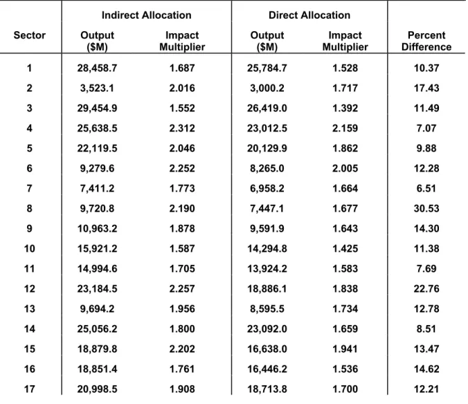
Applying formula (15) to an indirect allocation table will therefore produce erroneous results. Table 6 compares the economic significance, calculated using the direct allocation formula, of the 28 industries in the 1986-87 Australian economy using the direct allocation table (Table 11, ABS, 1990) and the indirect allocation table (Table 14, ABS, 1990). It shows that using the indirect allocation table in unadjusted form can significantly overestimate the impacts. For example, three industries show differences of over 20 percent (8:Clothing and footwear, 12:Petroleum and coal products, and 22:Repairs), while seventeen industries show differences of over 10 percent.
The implication of this is that in order to calculate multipliers or impacts from a table with indirect allocation of competing imports requires knowledge of the import coefficient matrix. Yet, in many cases (for example, some national tables produced for Indonesia, India or the United States), import matrices are not produced, or at least not published. This would appear to make the tables rather limited in their usefulness, unless some way can be found to estimate the import matrix. On possibility is to use the procedure adopted by the Australian Bureau of Statistics, namely to assume that "each using sector draws on imports and local production in the average proportions established for the total supply of each commodity" (ABS p.5).
9. IMPACT VERSUS EVALUATION STUDIES
At this stage, a note of caution regarding the distinction between impact analysis and evaluation studies. There is often some confusion in public discussion on the use of the terms 'impact' and 'evaluation'. Input-output analysis is concerned with measuring the impact or effect of a given stimulus on the economy in economic terms such as levels of output and employment. These impacts are represented simply as transactions; usually as increases or decreases in the value of
gross regional product. Because of the growth-orientation of economics and the general belief that growth is the desired objective, there is some implication attached to input-output analysis that an addition to transactions through an expanded or new industry in the table is a desirable development or benefit to the economy. While this implication is common, it can be somewhat misleading.
The benefit/cost approach to project evaluation attempts to demonstrate the relationship between the benefits derived by society and the costs (monetary or otherwise) induced as a result of an action or investment, i.e. whether society as a whole benefits from the project in question, in comparison to alternative uses for the resources available. Part of these streams of benefits and costs would appear in the input-output table where they are not separated as benefits and costs per se, but are simply transactions within the economy.
Table 6 Comparison of Industry Impacts Using Direct Import Allocation Procedures With Different Import Allocation Tables, Open Model, Australia, 1986-87
Indirect Allocation Direct Allocation
Sector Output
($M) Multiplier Impact Output ($M) Multiplier Impact Difference Percent
1 28,458.7 1.687 25,784.7 1.528 10.37 2 3,523.1 2.016 3,000.2 1.717 17.43 3 29,454.9 1.552 26,419.0 1.392 11.49 4 25,638.5 2.312 23,012.5 2.159 7.07 5 22,119.5 2.046 20,129.9 1.862 9.88 6 9,279.6 2.252 8,265.0 2.005 12.28 7 7,411.2 1.773 6,958.2 1.664 6.51 8 9,720.8 2.190 7,447.1 1.677 30.53 9 10,963.2 1.878 9,591.9 1.643 14.30 10 15,921.2 1.587 14,294.8 1.425 11.38 11 14,994.6 1.705 13,924.2 1.583 7.69 12 23,184.5 2.257 18,886.1 1.838 22.76 13 9,694.2 1.956 8,595.5 1.734 12.78 14 25,056.2 1.800 23,092.0 1.659 8.51 15 18,879.8 2.202 16,638.0 1.941 13.47 16 18,851.4 1.761 16,446.2 1.536 14.62 17 20,998.5 1.908 18,713.8 1.700 12.21
18 12,354.4 2.097 10,380.9 1.762 19.01 19 23,423.2 1.434 22,130.1 1.335 5.84 20 85,774.3 2.142 74,084.7 1.850 15.78 21 81,276.7 1.612 75,537.2 1.498 7.60 22 11,276.7 1.775 9,380.6 1.476 20.21 23 53,236.2 1.582 48,063.4 1.428 10.76 24 59,318.9 1.381 55,886.0 1.301 6.14 25 40,176.5 1.454 38,550.7 1.395 4.22 26 34,560.9 1.823 29,894.4 1.577 15.61 27 61,067.6 1.453 56,075.8 1.334 8.90 28 34,917.3 1.854 30,660.0 1.628 13.89
While it is important to draw this conceptual distinction between impact and evaluation studies, it is not uncommon to observe impact statements used as justification for a course of action. In fact, impact statements are often seen as ends in themselves, negating the need for an evaluation. However, while impact statements should provide important input into evaluation studies, they do not in themselves provide evaluative guidance from a benefit/cost point of view.
10. ASSUMPTIONS AND EXTENSIONS OF THE BASIC MODEL
This paper would not be complete without some mention of the assumptions inherent in the basic model. While the input-output table is simply an accounting statement, the transformation of the table into an operational model requires the use of a number of explicit assumptions.
The assumptions of the input-output model are concerned almost entirely with the behaviour of production. The model is based on the premise that it is possible to divide all productive activities in an economy into sectors whose interrelations can be meaningfully expressed as a simple set of equations. The crucial assumption is that the money value of goods and services delivered by an industry to other producing sectors is a linear and homogeneous function of the output level of the purchasing sector. More precisely, the specific assumptions are as follows:
(i) The inputs purchased by each sector are a function only of the level of output of that sector. The input function is generally assumed linear and homogeneous of degree one, which implies constant returns to scale and no substitution between inputs. The technology is also assumed constant.
production. This implies that there is only one method used to produce each commodity and that each sector has only a single primary output. In other words, there are no joint products.
(iii) The total effect of carrying on several types of production is the sum of the separate effects. This rules out external economies and diseconomies and is known simply as the additivity assumption.
(iv) the system is in equilibrium at given prices.
(v) In the static input-output model, there are no capacity constraints so that the supply of each good is perfectly elastic. Each industry can supply whatever quantity is demanded of it and there are no capital restrictions.
These assumptions highlight the desirable (and undesirable) features that ideally our model should possess. Thus, for example, the input coefficients are fixed average input propensities and we need to accept that each dollar increase in output results in the same proportional increase in inputs. This obviously rules out economies of scale. This distortion may not be excessive provided that the initial impact is small relative to the size of the industry in question and the overall economy. If however, the impacts involve a restructuring of local industries, input-output would not be appropriate. Similarly, we would want the model to be as disaggregated as possible, i.e. contain as many sectors as possible, to minimise the effects of error caused by a sector producing more than one product.
There are other implications too. The model assumes full employment with no capacity constraints, and thus prices have no role to play in the input-output model. Again, one needs to view the application in the light of these restrictions. If the area under study is a small open economy relative to the rest of the nation, where factors of production can easily move into and out of the region and local prices gravitate to external prices (subject to transport margins, etc.)14, then the input-output model would be a reasonable choice. Conversely, if the economy is closed and there is likely to be ‘crowding-out’ of factors, then a more complex model is required.
In terms of applied input-output analysis, the focus of these assumptions comes down primarily to three main points: the static nature of the model, the linearity property, and unlimited capacity. It is for these reasons that more sophisticated models have been developed. These models still retain input-output as a core component, but have become more complex, both in terms of trying to capture a wider subset of reality and in terms of their mathematical structure. It is not the intention of this paper to discuss these alternative models, other than to mention that they are 14 This is referred to as the ‘small country assumption’. It also implies that there is a question of aggregation
involved. If there is some product differentiation between local and imported commodities, this assumption becomes less viable.
available. They range from simple extensions, e.g. the extended activity-commodity framework (e.g. Miyazawa, 1976; Batey and Madden, 1981; Oosterhaven and Folmer, 1985) which retains the linear structure of the simple model, to computable general equilibrium (e.g. Shoven and Whalley, 1992; Dixon, et al., 1992) and integrated input-output/econometric models (e.g. Conway, 1990; West 1994) which are non-linear and differ in the manner in which they estimate the parameters. The former assumes various mathematical forms for supply and demand, e.g. CES production functions and Stone-Geary utility functions. The latter estimates the parameters directly using econometric functions. The former retains the static structure of the input-output model whereas the latter is more closely aligned with dynamic regional econometric models. Both incorporate supply restrictions through prices.
However, for small regional economies, it is unlikely that these more complex models will surpass the simpler input-output model. Notwithstanding the small country assumption, given the considerable difficulties associated with estimating a large number of coefficients and parameters when there is virtually no local data available, the increased ‘fuzziness’ may more than offset the increase in model sophistication. In such cases, the old maxim of ‘simple models for simple economies’ may be worth keeping in mind.
11. CONCLUSION
The methodology used in many studies involving input-output analysis appears to be often misdirected, particularly in the way multipliers are used. The preoccupation with multipliers has led to an abuse of the concept, to the extent that the multiplier often seems more important than the actual dollar or employment impact on the economy. This preoccupation has led in turn to incorrect analytical procedures in many studies; for example, it seems common practice to first derive a multiplier and then use this multiplier to calculate the total impact on the economy. This paper demonstrates that this approach is often erroneous and can result in significant errors.
Other issues which are often misunderstood include the use of output multipliers, state versus regional multipliers and impacts, expenditure switching and table balancing. These are but some of the pitfalls for the unwary analyst. Another factor in the empirical use of input-output tables, particularly in developing countries, is the availability of tables with suitable accounting format. Many developing countries, and some developed countries such as the United States, only publish tables with indirect allocation of imports. Such tables cannot be used for empirical analysis (in the usual multiplier of impact context) unless adjusted for imports. The dilemma is that import matrices are generally not published with the tables. This imposes an additional burden on the analyst, but unfortunately many analysis do not appear to be aware of the problem.
REFERENCES
Australian Bureau of Statistics (1990) Australian National Accounts: Input-Output Tables 1986-87, Cat.No. 5209.0.
Batey, P.W.J. and Madden, M. (1981) Demographic-Economic Forecasting Within an Activity-Commodity Framework: Some Theoretical Considerations and Empirical Results. Environment and Planning A, 13: pp.1067-1083.
Burke, R. (1984) Victorian Input-Output Table 1980/81, Information Paper No.1, Department of Industry, Commerce and Technology.
Burns, J.P.A., Hatch, J.H. and Mules, T.J. (eds.) (1986) The Adelaide Grand Prix - The Impact of a Special Event, Centre for South Australian Economic Studies, Adelaide.
Conway, Jr., R.S. (1990) The Washington Projection and Simulation Model: A Regional Interindustry Econometric Model. International Regional Science Review, 13: pp. 141-165. Dixon, P.B., Parmenter, B.R., Powell, A. and Wilcoxen, P. (1992) Notes and Problems in Applied General Equilibrium Models, Elsevier, Amsterdam.
Groenewold, N., Hagger, A.J. and Madden, J.R. (1987) The Measurement of Industry Employment Contribution in an Input-Output Model. Regional Studies, 21(3): pp 255-263. GSO (1995) Input-Output Analysis and Economic Impact Assessment within the Queensland Public Sector, Queensland Government Statistician's Office, Brisbane.
Miller, R.E. and P.D. Blair (1985) Input-Output Analysis: Foundations and Extensions, Prentice-Hall, Inc., Englewood Cliffs, New Jersey.
Miyazawa, K. (1976) Input-Output Analysis and the Structure of Income Distribution, Springer, Berlin.
Oosterhaven, J. and Folmer, H. (1985) An Interregional Labour Market Model Incorporating Vacancy Chains and Social Security. Papers of the Regional Science Association, 58: pp. 141-155.
Shoven, J.B. and Whalley, J. (1992) Applying General Equilibrium, Cambridge University Press, Cambridge.
West, G.R. (1994) The Queensland Impact and Projection Model: The Household Sector.