Junior Management Science
journal homepage:www.jums.academyAdvisory Editorial Board:
DOMINIK VAN AAKEN FREDERIK AHLEMANN CHRISTOPH BODEROLF BRÜHL JOACHIM BÜSCHKEN LEONHARD DOBUSCHRALF ELSAS DAVID FLORYSIAK GUNTHER FRIEDL WOLFGANG GÜTTEL CHRISTIAN HOFMANN KATJA HUTTER LUTZ JOHANNING STEPHAN KAISER ALFRED KIESER NATALIA KLIEWER DODO ZU KNYPHAUSEN-AUFSEßSABINE T. KÖSZEGI ARJAN KOZICA TOBIAS KRETSCHMER HANS-ULRICH KÜPPER REINER LEIDL ANTON MEYER MICHAEL MEYER GORDON MÜLLER-SEITZ J. PETER MURMANN BURKHARD PEDELL MARCEL PROKOPCZUK TANJA RABL SASCHA RAITHEL ASTRID REICHEL KATJA ROST MARKO SARSTEDT DEBORAH SCHANZ ANDREAS G. SCHERERSTEFAN SCHMID UTE SCHMIEL CHRISTIAN SCHMITZ PHILIPP SCHRECK GEORG SCHREYÖGGLARS SCHWEIZER DAVID SEIDL THORSTEN SELLHORN ANDREAS SUCHANEK ORESTIS TERZIDIS ANJA TUSCHKE SABINE URNIK STEPHAN WAGNER BARBARA E. WEIßENBERGERISABELL M. WELPE HANNES WINNER CLAUDIA B. WÖHLETHOMAS WRONA THOMAS ZWICK
Volume 4, Issue 3, September 2019 JUNIOR MANAGEMENT SCIENCE Belinda Kellerer,AversionPortfolio Optimization and Ambiguity
Tobias Wulfert,Mobile App Service Quality Dimensions and Requirements for Mobile Shopping Companion Apps
Virginia Springer,Bewertung der Übertragbarkeit von neuronalen Studienergebnissen auf einen Accounting-Kontext
Lukas Ferner,Measuring the Impact of Carbon Emissions on Firm Value Using Quantile Regression
Leona Schink,Die Legitimation einer Innovation durch Cultural Entrepreneurship – Explorative Fallstudie eines symbiotischen Zusammenspiels zwischen einem Start-up und dessen Schlüsselkunden
Annalena Düker,Das Management von Produktrückrufen: Einflussfaktoren auf die Rückholung von Verbraucherprodukten 305 339 392 422 433 460
Published by Junior Management Science e.V.
Portfolio Optimization and Ambiguity Aversion
Belinda Kellerer
Ludwig-Maximilians-Universität München
Abstract
This thesis analyses whether considering ambiguity aversion in portfolio optimization improves the out-of-sample performance of portfolio optimization approaches. Furthermore, it is assessed which role ambiguity aversion plays in improving the portfolio performance, especially compared with the role of estimation errors. This is done by evaluating the out-of-sample performance of the approach of Garlappi, Uppal and Wang for an investor with multiples priors and aversion to ambiguity compared to other portfolio optimization strategies from the literature not taking ambiguity aversion into account. It is shown that considering ambiguity aversion in portfolio optimization can improve the out-of-sample performance compared to the sample based mean-variance model and the Bayes-Stein model. However, the minimum-variance model and the model of naïve diversification, which are both independent of expected returns, outperform the approach considering ambiguity aversion for most of the empirical applications shown in this thesis. These results indicate that ambiguity aversion does play a role in portfolio optimization, however, estimation errors regarding expected returns overshadow the benefits of optimal asset allocation.
Keywords: portfolio choice; asset allocation; estimation error; ambiguity; uncertainty.
1. Introduction
1.1. Problem definition
The classical mean-variance portfolio optimization ap-proach, established by Harry Markowitz, is based on the assumption that expected asset moments are known. In real-life investment decisions, these input parameters are, however, unknown and need to be estimated. Typically, the input parameters are estimated from realized returns and as a result, they are inevitably estimated with error. This is particularly important because the choice of input parame-ters has a huge effect on the optimal portfolio weights and consequently on the portfolio performance. As these estima-tion errors are ignored in the classical portfolio optimizaestima-tion approach, a bad out-of-sample performance is the result. Mean-variance optimized portfolios often show a low de-gree of diversification and extreme portfolio weights1. To improve the performance of the classical mean-variance ap-proach, new methods were developed that explicitly take into account that the estimated asset moments are not the true values. In this context, a very important class of methods
1See for exampleHodges and Brealey(1973),Best and Grauer(1991)
andBlack and Litterman(1992)
is the class of Bayesian approaches. Using these approaches, the input parameters are adjusted before they are used to determine the optimal portfolio. This is done by combining a priori information with the historical data by the means of Bayesian updating. Empirical studies have shown that these adjustments lead to a better out-of-sample performance (e.g.
Jorion,1986).
Bayesian approaches, however, assume that the proba-bility distribution of outcomes is known and the decision-maker has a unique prior for the outcomes, while it is ig-nored that this is not the only possible probability distribu-tion. From the uncertainty about the true probability distri-bution, a new type of uncertainty arises, called ambiguity. In this thesis, ambiguity is defined as Knightian uncertainty (Knight,1921), which refers to uncertainty that can’t be mea-sured because the probability distribution is unknown and risk refers to measurable uncertainty with a known proba-bility distribution. In 1961, Ellsberg was the first to show experimentally that investors are averse against this type of uncertainty (Ellsberg,1961). He showed that the majority of investors prefer a risky investment to an ambiguous invest-ment. A central Bayesian assumption is that all uncertainties can be reduced to risks. This assumption, however, contra-dicts Ellsberg’s empirical results. If an investor is ambiguity
averse, his behavior in the Ellsberg experiment leads to a vio-lation of Savage’s subjective expected utility theory (Savage,
1954), because the sure-thing-principle is disobeyed. There-fore, ambiguity averse behavior is not rational according to subjective expected utility theory. As a consequence, new portfolio optimization models were developed that allow for ambiguity aversion by weakening the sure-thing principle2.
In the center of this thesis is the multi-prior approach introduced by Garlappi et al. (2007). They developed an approach that takes both, parameter uncertainty about the true asset moments and ambiguity aversion into considera-tion. They did so by extending the classical mean-variance approach by two main points. Firstly, they implement an additional constraint on the expected return for each asset to lie within a confidence interval of the estimated expected return. Secondly, they apply an additional minimization over the choice of possible expected returns. Ambiguity aversion is implemented by this additional minimization. Furthermore, the model of Garlappi, Uppal and Wang is also able to account for model uncertainty. This is in case the investor forms his beliefs about expected returns from a factor model, like the Capital Asset Pricing Model (CAPM), but is unsure whether this factor model is the true return-generating model. Garlappi, Uppal and Wang present in their empirical study, that accounting for ambiguity aver-sion, when optimizing portfolios, improves the portfolio per-formance and leads to a higher out-of-sample Sharpe ratio compared to the classical mean-variance approach and the Bayes-Stein approach.
This thesis focuses on the question whether the out-of-sample performance can be improved if ambiguity aversion is considered in portfolio optimization, and which role am-biguity plays in improving the portfolio performance. To an-swer these questions, an empirical study is performed to com-pare the performance of the ambiguity-averse approach in-troduced by Garlappi, Uppal and Wang with the performance of several other models from the literature, like the classi-cal mean-variance model, the minimum-variance model, the Bayes-Stein model and the model of naïve diversification. Additionally, the results are tested for robustness by vary-ing important model assumptions. In this way, it is analyzed which additional value can be generated by taking ambigu-ity aversion into consideration. It is of particular interest which role ambiguity aversion plays compared with the role of estimation errors. Furthermore, the relationship between risk aversion and ambiguity aversion is analyzed and its role for the optimal portfolio is discussed. Besides investigating the effect of ambiguity aversion on the out-of-sample perfor-mance of optimized portfolios, a critical view is taken on the topic. Crucial issues, like the rationality of ambiguity averse investment decisions and learning under ambiguity, are dis-cussed.
2See for exampleSchmeidler(1989) andGilboa and Schmeidler(1989)
1.2. Method of investigation
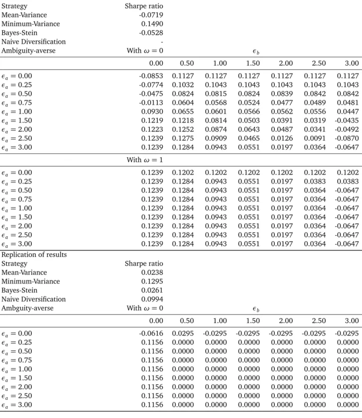
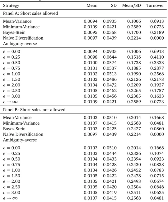
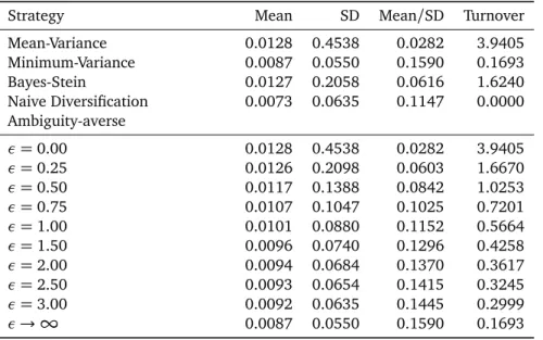
To analyze the effect of ambiguity averse investment de-cisions on the portfolio performance, an empirical study is performed. This empirical study is based on the work of Gar-lappi, Uppal and Wang and is divided into three parts. In the first part, the original results of Garlappi, Uppal and Wang are replicated with a special focus on differences in results. With regard to this empirical application, the investor can build his portfolio from eight international equity indices. In the second part, important input parameters like the sample size to determine the optimal portfolio weights, the degree of risk aversion and the timespan are varied. Finally, in the third part of the empirical study, the investment universe is changed and the portfolio optimization problem is applied to the German DAX30 stocks. Most assumptions are thereby taken from Garlappi, Uppal and Wang to ensure the com-parability of the results. This empirical design is chosen to show whether incorporating ambiguity aversion to the port-folio optimization problem leads to a better out-of-sample performance independent of the framework conditions. Fur-thermore, the variation of input parameters ensures that the improved out-of-sample performance results from taking am-biguity aversion into account and not from other character-istics, for example time-specific or asset-specific characteris-tics.
The rest of this thesis is organized as follows. In Chap-ter 2, the foundations of modern portfolio theory are pre-sented and the problems arising from the classical mean-variance approach are discussed. Subsequently, suggestions for improvement, like imposing additional constraints or us-ing Bayesian approaches, are examined. Chapter 3 gives a critical literature overview regarding ambiguity aversion in the context of portfolio optimization. In Chapter 4, the ambiguity-averse approach introduced by Garlappi, Uppal and Wang, which takes ambiguity aversion as well as param-eter and model uncertainty into account, is presented. Chap-ter 5 describes the empirical applications and illustrates the out-of-sample performance of different portfolio optimiza-tion strategies in an empirical study by first replicating the original results of Garlappi, Uppal and Wang and then chang-ing important framework conditions. The conclusion is pre-sented in Chapter 6. Further illustrations are collected in the Appendix.
2. Portfolio choice
2.1. Modern portfolio theory
More than 60 years ago, Harry Markowitz established a whole new concept of portfolio optimization by focusing on a holistic approach of several assets to build a portfolio rather than to restrict the investment to a single seemingly prof-itable asset. In his article “Portfolio selection” of 1952, he derived a normative decision rule to build efficient portfo-lios. With this decision rule, he laid the foundation for a the-ory, which was later called modern portfolio theory. About 40
years later, in 1990, Harry Markowitz won the Nobel prize to-gether with Merton H. Miller and William F. Sharpe for their pioneering work in the theory of financial economics3.
According to Markowitz an investor should focus on two main elements when selecting the optimal portfolio, namely portfolio return and portfolio risk, where risk is defined as fluctuations in returns. He argues that each investor has different interests when choosing a portfolio, but every in-vestor pursues the goal to achieve high returns at low risk. “It seemed obvious that investors are concerned with risk and return, and that these should be measured for the portfolio as a whole” (Markowitz, 1991, p. 470). Modern portfolio theory is based on the assumption that investors are only willing to hold a risky asset if they are compensated with a risk premium in addition to the return on the risk-free asset. Therefore, Markowitz implicitly assumes that investors are risk averse.
To determine the portfolio risk, it is important to analyze the correlations between the assets. If assets are not per-fectly correlated with each other, it is possible to reduce the portfolio risk through diversification, without reducing the expected return. As a result, the portfolio risk is always be-low the weighted average of the individual assets’ risk. As the number of assets in the portfolio increases, the role of the co-variances becomes more important compared to the role of the variances of the single assets. The direct implication of this concept for the optimal portfolio is that “it is necessary to avoid investing in securities with high covariances among themselves” (Markowitz,1952, p. 89).
Modern portfolio theory is based on numerous assump-tions about the investor and the market. Besides the key as-sumption that investors seek to maximize yields while min-imizing risk, Markowitz assumes that markets are efficient, that investors are rational and expected utility maximizers according to Bernoulli and that they make their decisions based on an individual risk function. Furthermore, the plan-ning horizon in modern portfolio theory covers only one pe-riod. At the end of each period the investor has to make a new decision about the allocation of his capital. Asset allo-cation according to Markowitz is therefore a static decision with a short-term character.
In his article of 1952, Markowitz distinguishes two ma-jor steps to determine the optimal portfolio. The first step is to form expectations about future asset moments and the second step is to specify the optimal portfolio. His model is limited to the second step, which can further be divided into identifying the set of efficient portfolios and identifying the investor-specific optimal portfolio using the concept of Bernoulli expected utility maximization. From the expecta-tions about future asset moments, the set of efficient portfo-lios is built. According to modern portfolio theory, a portfolio is efficient if there is no other portfolio with a higher expected return given a specific level of risk or with a lower risk given a specific level of expected return. All portfolios that are
ef-3For further information see Nobelprize.org
ficient lie on the efficient frontier, which represents the re-lationship between risk and return. In an efficient portfolio, assets with high expected returns, small variances and low correlation coefficients among each other are the ones with the highest weights. After determining the set of efficient portfolios, the next step is to select the investor-specific opti-mal portfolio depending on his degree of risk aversion. The optimal portfolio can be derived as the point of tangency be-tween the efficient frontier and the highest possible Bernoulli utility curve. According to Markowitz, the optimization prob-lem given N risky assets can be written as:
max w w Tµ −γ 2w TΣw (1)
in whichwis the vector of portfolio weights,µis the vec-tor of returns,γis the investor-specific degree of risk aversion andΣis the variance-covariance matrix.
Markowitz, however, only analyzed how to identify the optimal portfolio given the information about future asset moments, but not how these input parameters can be deter-mined. Since information about future asset moments is un-known, the input parameters need to be estimated. Expected asset moments are typically estimated from realized returns and therefore, they are inevitably estimated with error. As opposed to that, in modern portfolio theory it is assumed that expected returns are known and as a consequence, statisti-cal estimations are assumed to be the true values (Kalymon,
1971).Hodges and Brealey(1973) andJorion(1985), how-ever, show in empirical studies that historical returns only have a small forecasting power for future returns. Addition-ally, Kempf et al. (2002) expose in their simulation study that the estimated expected returns differ significantly from the “true” values. They also show that there is a huge gap between the optimal portfolio weights using the “true” pa-rameters and using their estimations from historical returns. Therefore, they argue, that a rational investor should take un-certainty about estimated asset moments into account when selecting a portfolio. Barry(1974) shows that if uncertainty about future asset moments is integrated to the model, the portfolio risk can be reduced while leaving the portfolio re-turn unchanged, leading to increasingly efficient portfolios.
Chopra et al.(1993) argue that the estimation of variances and covariances can be performed more precisely than the estimation of expected returns but at the same time, estima-tion errors in returns have a much higher quantitative influ-ence on the portfolio weights and the resulting portfolio per-formance compared to estimation errors regarding variances and covariances. Therefore, they conclude that the focus of the estimation should lie on expected returns.
One of the main drawbacks of modern portfolio theory is, that the resulting optimal portfolios are often characterized by instable portfolio weights and by extreme, non-intuitive positions (Black and Litterman,1992). A small increase in the expected return of only one asset already leads to the re-allocation of half of all assets in the portfolio, while the port-folio risk and return hardly change (Best and Grauer,1991).
This result is not consistent with the investors’ preference to allocate capital to stable portfolios that don’t require fre-quent reallocations, since reallocations are associated with high transaction costs. Furthermore, using mean-variance optimization, the capital is allocated only to a few assets, leading to undiversified portfolios (Black and Litterman,
1992, Green and Hollifield, 1992, Broadie, 1993). These extreme portfolio weights conflict with the desire of diver-sification. Finally,Jobson and Korkie(1980) andDeMiguel et al. (2009) show that the optimal portfolio selected, us-ing mean-variance optimization, can be even beaten by a uniformly diversified portfolio regarding the Sharpe ratio.
Michaud(1989) argues that the classical mean-variance approach puts high weights on assets with high expected returns, small variances and low covariances among each other, but at the same time, assets with these characteris-tics are often afflicted with the highest estimation errors. Therefore, assets with highly overestimated returns and with highly underestimated variances are overweighted in the op-timal portfolio. This leads to an increase of the estimation error through optimization. For this reason, Michaud among others states that mean-variance portfolio optimization is “er-ror maximization”. To solve this problem, Michaud suggests an alternative, statistical, approach to estimate future asset moments. Michaud argues that the observable historical data represents only one realization of the data-generating pro-cess. Therefore, he proposes to reestimate the return distri-bution using Monte Carlo Simulation. From each simulated return distribution, a new set of input parameters for the sub-sequent optimization arises, leading to resampled efficient portfolios. Scherer(2003), however, criticizes the approach suggested by Michaud because it does not solve the cause of the bad out-of-sample performance of mean-variance port-folios induced by estimation errors regarding expected asset moments. Each portfolio, which is constructed during the simulation, is derived using the same input data. As a re-sult, every resampled efficient portfolio has a similar devia-tion from the “true optimal portfolio” (Scherer,2003). Fur-thermore,Fletcher and Hillier(2001) compared the perfor-mance of resampled efficient portfolios with the perforperfor-mance of classical mean-variance portfolios and they don’t find any outperformance of either strategy.
Since the bad out-of-sample performance of mean-variance portfolios arises from estimation errors associated with expected asset moments (Merton, 1980), alternative approaches that are explicitly designed to reduce estimation errors, were established. In the following Chapters, differ-ent suggestions for improvemdiffer-ent, like setting up additional constraints or adjusting the input parameters by the means of Bayesian approaches are analyzed and compared. 2.2. Implementation of additional constraints
Since different out-of-sample studies have shown that portfolios that are optimized using the classical mean-variance approach tend to be very undiversified, additional constraints can be introduced to force a higher diversifica-tion. Examples of constraints include the restriction of short
selling, upper bound constraints on the position in a single asset or upper bound constraints on the exposure given to a certain country or industry (Brandt, 2009). Often, these restrictions are necessary because of legal requirements and therefore, constraints are a realistic assumption. Introduc-ing additional constraints limits the set of possible portfolio combinations, leading to an efficient frontier that always lies below the non-restricted efficient frontier. As a result, adding constraints can never improve the ex-ante portfo-lio performance (Grauer and Shen,2000). However, it has been shown that the out-of-sample portfolio performance can be improved. Restricting portfolios has a smoothening effect on portfolio weights, leading to a higher degree of diversification and to less extreme asset positions (Grauer and Shen,2000). In a simulation study,Frost and Savarino
(1988) show that introducing short selling constraints and upper bound constraints on assets improves the portfolio performance. They measure performance using certainty equivalent returns, which is the difference in portfolio utili-ties, if the portfolio weights are based on estimated returns and if they are based on the true parameters. Frost and Savarino conclude that the implementation of constraints is reasonable if estimated asset moments are afflicted with esti-mation errors. This is because the use of constraints prevents the inappropriate emphasis of estimation errors in portfolio optimization (Chopra and Ziemba,1993).
If estimation errors, however, are not the cause of badly diversified portfolios, constraints are counterproductive, since they predetermine the optimal portfolio to a large ex-tent ex-ante. This fact is criticized by Banz, as he states that constraints are implemented “to force the results which one desires” (Banz,1997, p. 398). Clasing and Rudd(1988) also argue that implementing constraints is counterproductive. They state that adding restrictions implies that the investor doesn’t trust the input parameters. Therefore, they conclude that it is more intuitive to directly adjust the input param-eters instead of implicitly changing them by implementing constraints. Grinold and Easton (1998) agree and argue that implementing constraints doesn’t treat the cause of the bad out-of-sample performance of mean-variance optimized portfolios.
Out-of-sample studies have shown that the portfolio per-formance can be improved by implementing constraints, but the performance is still far from good. The reason for this re-sult is that estimated asset moments are afflicted with estima-tion errors that are so high that the adjustment of the optimal portfolio by adding constraints is not sufficient to solve this problem (Brandt,2009). To overcome the counterintuitive approach of restricting the outcome by implementing con-straints, new techniques have been introduced that directly adjust the input parameters. One important class of these approaches is the class of Bayesian approaches, presented in the next Chapter.
2.3. Bayesian approaches 2.3.1. statistics
The founder of Bayesian statistics is Thomas Bayes (1702-1761). The Bayes’ theorem, that was developed by him, is a fundamental theorem in the theory of probability. Bayes’ rule describes the probability of an event based on prior knowl-edge, where P(A)is the prior, the initial degree of belief in
AandP(A|B)is the posterior, the degree of belief inAafter accounting forB. Bayes’ rule can be written as follows:
P(A|B) = P(B|A)P(A)
P(B) . (2)
In the course of portfolio optimization, the basic idea of using Bayes’ rule is, to combine a priori available information with the data to determine the posterior distribution of re-turns. These returns are then subsequently used for portfolio optimization. A priori information may result from financial research, news, events, macroeconomic analysis or asset pric-ing theories (Avramov and Zhou,2010). A basic assumption when using Bayesian approaches in portfolio optimization is that returns are independent and identically distributed vari-ables4. In the context of portfolio optimization, Bayes’ rule can be written as follows (Gelman et al.,1995):
P(θ|z) =R P(z|θ)P(θ) P(θ)P(z|θ)dθ =
P(z|θ)P(θ)
P(z) (3)
in whichz = (z1,z2,z3, . . . ,zt)is a vector of realized re-turns andθ represents the unknown parameters of the prob-ability distribution. The value ofθ shall be estimated by the means of Bayesian statistics. Bayesian statistics considersθ a random variable. Information that is known ex ante about
θ is combined in the a priori probability distribution P(θ). This a priori distribution is then combined with the informa-tion from the historical sample to form the a posteriori dis-tributionP(θ|z). In contrast to methods of classical statistics where it is assumed thatθ=thet aˆ and therefore a point es-timate ofθ is provided and any potentially relevant prior in-formation is disregarded, Bayesian statistics provides a whole distribution ofθ. As a consequence, it is possible to directly quantify the uncertainty aboutθ (Gelman et al.,1995). To solve portfolio optimization problems, it is necessary to esti-mate future asset returnsz. This is done by the forecasting distribution P(ˆz|z), in which ˆz is the estimated value of z. The forecasting distribution results from the likelihood func-tion of a future observafunc-tionP(ˆz|θ) and the a posteriori distri-bution P(θ|z). Using Bayesian statistics, the distribution of future expected returns is derived by integrating over all pos-sible values ofθ weighted with their respective a posteriori probabilities (Gelman et al.,1995):
P(ˆz|z) =
Z
P(ˆz,θ|z)dθ=
Z
P(ˆz|θ)P(θ|z)dθ (4)
4See for exampleJorion(1986),Black and Litterman(1992) andPástor
(2000).
Already during the 1970s, the idea to use Bayesian statis-tics to account for estimation errors in portfolio optimization was developed byBarry(1974) andKlein and Bawa(1976). Unlike implementing constraints, Bayesian approaches ex-hibit a decision-theoretical fundament. If a Bayesian ap-proach is applied, the adjustment of the optimal portfolio takes place by directly changing the input parameters. In this way, the problem of estimation errors is directly ad-dressed. The adjusted input parameters are then used for portfolio optimization. Barry and Klein and Bawa assume a non-informative diffuse a priori distribution, which means that they assume that all values for the future returns are con-sidered equal probable a priori. As estimation errors are inte-grated in the Bayesian framework, assets are riskier since pa-rameter uncertainty is an additional source of risk (Avramov and Zhou,2010). As a result, in the studies of Barry and Klein and Bawa, the vector of expected returns remains un-changed but the variance-covariance matrix is multiplied by 1+1/n, in which nis the sample size. Consequently, if a non-informative prior is used, the set of efficient portfolios doesn’t change, but the investor chooses a portfolio further to the left on the efficient frontier compared to the optimal portfolio under the classical mean-variance approach.
Brown(1976) concludes that using Bayesian approaches leads to quantifiable different portfolio structures. He adds that the results, however, depend strongly on the choice of the prior. If a non-informative prior is used, as done by Barry and Klein and Bawa, the only difference to the mean-variance approach is the multiplication of the variance-covariance ma-trix with the factor 1+1/nand therefore, the effect on the optimal portfolio is very small if the sample sizenis large. Ifn
is very large, the effect is so small that the optimal portfolio is almost identical to the optimal portfolio under the classical mean-variance approach. Avramov and Zhou(2010) state that, for all practical sample sizes, the effect of diffuse priors is negligible and therefore, in order to exploit the decisive advantage of the Bayesian approaches, it is necessary to gain informative priors for example from events, macro conditions or asset pricing theories.
2.3.2. Shrinkage estimators
Shrinkage estimators go back to Charles Stein et al.
(1956). Stein points out that the sample mean is not an optimal estimator for the mean of a multivariate normal dis-tributed random variable. He argues, that if expected asset returns are estimated from the sample mean, the value is based solely on the return history of the particular asset and other potential information from the return histories of other assets are disregarded. To overcome this weakness, Stein de-veloped an estimator that includes the return histories of all assets to determine expected returns, leading to more precise results. Stein shrinks the sample mean of each asset towards the overall sample mean of all assets, the “grand mean”. This approach has a smoothening effect and prevents extreme val-ues because expected returns of assets with comparably high or low past returns are strongest shrunk towards the grand mean. The key element of the Stein estimator is the
shrink-age factor, which determines how strong the sample means are shrunk towards the grand mean. The general form of the Stein estimator (James and Stein,1961) can be written as follows:
¯
rj(φ) =φr0+ (1−φ)¯rj (5) in which φ is the shrinkage factor, r0 is the shrinkage target, ¯rj is the sample mean of asset jand ¯rj(φis the ad-justed weighted mean of asset j. The shrinkage factor in-creases in the number of assets N, decreases in the length of the sample size nand decreases in the distance between the sample mean and the shrinkage target. Shrinkage es-timators are, for example, used by Jobson (1979), Jorion
(1986),Frost and Savarino(1986) andChopra et al.(1993). Chopra, Hensel and Turner suggest a global index as shrink-age target and show that a weighted avershrink-age of the individual asset mean of each country and the global index is a supe-rior estimator of the true asset mean for each country. Frost and Savarino specify an informative prior and assume that all assets have a priori identical expected means and vari-ances and that the pairwise correlation coefficient between any two assets is the same. They shrink the estimates of each assets’ expected return, variance and pairwise correlation co-efficient, determined from the historical sample, towards the average return, average variance and average correlation co-efficient of all assets within the population. Therefore, the approach leads to a shrinkage towards the equal weighted portfolio and the degree of shrinkage depends on the de-gree to which the sample is consistent with the shrinkage target. Frost and Savarino argue that parameters with large discrepancies between the sample estimate and the overall mean of that parameter are more likely to contain estima-tion errors and those values are adjusted strongest towards the grand mean, reducing the estimation error. The authors show that the portfolio performance can be improved by ap-plying their informative prior compared to apap-plying an unin-formative prior or the classical mean-variance approach.
Jagannathan and Ma(2003) point out that certain con-straints that were discussed in Chapter 2.2 can be interpreted in a similar way as shrinkage estimators. They show that no short sales constraints are equivalent to reducing the es-timated covariances and that upper bound constraints are equivalent to increasing the respective estimated covari-ances. Although the effect of both methods can be very similar, the motivation is different. While imposing con-straints restricts the outcome exogenously, the adjustment of the input parameters when using shrinkage estimators is endogenous.
2.3.3. Bayes-Stein estimator
Jorion(1985) introduced the Bayes-Stein estimator, a fur-ther development of the classical Stein estimator. In con-trast to Frost and Savarino, he assumes that estimation errors regarding the variance-covariance matrix are negligible and that variances can be estimated directly from the historical
sample. Jorion argues that the minimum-variance portfolio is the only portfolio on the efficient frontier that is free of estimation errors since the determination of the minimum-variance portfolio depends solely on the minimum-variance-cominimum-variance matrix, which is assumed to be known. The more the in-vestor moves to the right on the efficient frontier, the larger is the influence of estimation errors regarding expected re-turns. Therefore, the idea of Jorion is to shrink the mean-variance portfolio towards the minimum-mean-variance portfolio, since it is robust to uncertainty about expected means and at the same time it is associated with the least risk. Using the Bayes-Stein shrinkage estimator, the sample means of the in-dividual assets are shrunk towards the mean of the minimum-variance portfolio. The intensity of the shrinkage depends on the sample size n and on the precision of the sample meanv. The shrinkage factorφcan be computed as follows (Jorion,
1986): φ= v n+v (6) withv= N+2 (¯r−r01)TΣ−1(¯r−r 01) (7) in which N is the number of assets, r0 is the shrinkage target and ¯r is the sample mean. The shrinkage factorφis then inserted into (5) to obtain the weighted average mean for the individual asset. Since the values forφ andr0 are determined directly from the sample, this approach is also called an empirical Bayes approach.
If the Bayes-Stein estimator is used to determine the opti-mal portfolio, the efficient frontier and the portfolio weights of the efficient portfolios don’t change, but the investor will choose a portfolio more to the left on the efficient frontier, closer to the minimum-variance portfolio (Jorion,1986). Jo-rion concludes that using the Bayes-Stein shrinkage estimator leads to a significantly improved out-of-sample performance.
Chopra et al.(1993) confirm this result. 2.4. Model Uncertainty
The approaches, that have been introduced in Chapter 2.3.2 and 2.3.3, dealt with the adjustment of the sample as-set moments by shrinking them towards a grand mean, by the means of Bayesian statistics. All approaches presented in the previous Chapters have in common, that solely the histor-ical sample is used as input data to determine expected asset moments. Findings from asset pricing theory haven’t been taken into account so far. In this Chapter, an alternative ap-proach to estimate expected asset moments based on factor models is presented.Chan et al.(1999) show that using fac-tor models to determine the input parameters for portfolio optimization significantly improves the performance of the resulting portfolios. They add, that the resulting portfolios also show a higher degree of diversification compared to a solely data-driven approach.
Pástor (2000) and Pástor and Stambaugh (2000) ar-gue that if expected asset moments are determined exclu-sively from historical returns, potential information from asset-pricing models are ignored. They developed the data and model approach, in which they combine information from historical data with implications from the CAPM by the means of Bayesian statistics. They define a distinction of cases, withω=0 meaning the investor does not believe in the return-generating model andω=1 meaning the investor believes dogmatically in the CAPM, whereωcan take values between 0 and 1. In the data and model approach, the sam-ple means are shrunk towards the market portfolio and the degree of shrinkage depends on the shrinkage factor. The shrinkage factor measures the importance that is assigned to the CAPM and depends on the investors beliefs in the validity of the CAPMωand on how well the historical returns can be explained by the CAPM (Pástor,2000). Pastor and Pastor and Stambaugh argue that the investor’s uncertainty about the models pricing ability can be represented by an informative a priori distribution of Jensen’s alpha. If the a priori distri-bution of Jensen’s alpha is located around zero, there is only a low degree of uncertainty and the optimal portfolio will be close to the market portfolio. If the a priori distribution of Jensen’s alpha, however, is diffuse, the investor is highly uncertain about the models pricing ability and the optimal portfolio is mainly based on realized returns.
When comparing different factor models, Chan et al.
(1999) show that no clear favorite specification emerges. A simple single factor model like the CAPM can’t be es-sentially outperformed by a complex multi-dimensional k-factor model. Although the CAPM performs quite well in the study of Chen et. al., it can’t capture all of the covariation among assets which could result in a systematically biased estimate of asset moments (Brandt, 2009). Consequently, the difficulty of implementing a factor model in practice is the choice of factors, since there are huge disagreements among researchers about the predictability of returns. Fi-nancial economists have identified several economic vari-ables that predict future asset returns. However, there are large disagreements about the “true” predictive regression specification. These disagreements lead to a major source of uncertainty – model uncertainty (Avramov and Zhou,2010). If the estimation of asset moments is based on assumptions that don’t correspond with reality, estimation errors occur be-cause of model uncertainty. The focus on one single model fails to include model uncertainty and therefore the overall uncertainty is underestimated (Cremers,2002). If posterior odds ratios are used to rank several models and only the best model is used, it is implicitly assumed that the chosen model is true with a unit probability and model uncertainty isn’t considered. Subsequently, insights from all other models are completely ignored resulting in a loss of important informa-tion (Brandt, 2009). Pástor (2000) adds that in general a model will neither be a complete reflection of reality nor will it be completely useless.
In Chapter 2.3, Bayesian approaches were introduced that incorporate parameter uncertainty by generating a
weighted average of the data and the prior. This approach will now be extended to incorporate model uncertainty to portfolio optimization by implementing a weighted average of the competing return-generating models. Taking model uncertainty into account means that not only parameters, but also models, are implemented using probability distribu-tions (Hoeting et al.,1999). The Bayesian model averaging approach (BMA), presented byHoeting et al.(1999) deter-mines posteriori probabilities to a set of competing models and then these probabilities are used as weights for the re-spective model to form an overall composite model. This overall model is then used to solve portfolio choice prob-lems. The weights depend on the ability of the model to fit the data and on prior beliefs in the model (Hoeting et al.,
1999;Raftery et al.,1997). In this context, a Bayesian ap-proach is preferred because it allows to directly incorporate model uncertainty and is robust to model misspecification (Avramov and Zhou,2010). Model averaging leads to higher estimates of variances compared to approaches that don’t ac-count for model uncertainty. This is why ignoring model uncertainty leads to overconfident decisions (Nigmatullin,
2003). Avramov (2002) and Cremers (2002) each intro-duce a Bayesian model averaging approach which integrates out both, parameter and model uncertainty. In this context, Avramov states that investors who ignore model uncertainty suffer from significant utility losses. He shows for six portfo-lios over the time period 1953 to 1998, that the composite model outperforms the individual model with the highest posterior probability for any model selection criterion used. Cremers stresses the high importance of taking model un-certainty into account and shows that BMA provides an improved forecasting ability compared to model selection approaches. Anderson and Cheng (2016) develop a BMA approach in which the investor updates the probabilities of each model after every period using Bayes’ rule. They con-clude that accounting for model uncertainty improves the out-of-sample portfolio performance.
3. Ambiguity aversion
3.1. Concept of ambiguity aversion 3.1.1. A definition of ambiguity
It is well known that agents are risk averse and are will-ing to sacrifice expected return in order to reduce risk. But what is meant by risk? Knight(1921) was the first to note that not all sources of uncertainty can be quantified prob-abilistically and therefore risk is radically different from un-certainty. Knight distinguishes between two different types of uncertainty. Risk is referred to situations in which the proba-bilities of the outcomes are known, whereas ambiguity is re-ferred to situations in which the probability distribution is un-known. Ambiguity might occur because the decision maker is unable or unwilling to summarize the available information by a unique probability distribution, due to a lack of infor-mation.
3.1.2. The Ellsberg-experiment
While Knight was the first to differentiate between risk and ambiguity, Ellsberg(1961) was the first to show in his experiments that decision makers behave ambiguity averse.
In his first two-color urn-experiment there are two urns with 100 balls each. Urn1 contains exactly 50 red balls and 50 black balls while Urn2 also contains 100 balls, but the distribution of red balls and black balls is unknown and all combinations, ranging from 100 red balls and 0 black balls to 0 red balls and 100 black balls, are possible. Urn1 is a risky urn since the probability distribution is known. Urn2, however, is an ambiguous urn because the decision maker is unable to form a unique prior distribution over Urn2 with certainty, due to a lack of information. Decision makers were then asked whether they preferred (i) to bet on a red ball from either Urn1 or Urn2 and whether they preferred (ii) to bet on a black ball from either Urn1 or Urn2. In Ellsberg’s experiment, most decision makers preferred a bet on a red ball from Urn1 to a bet on a red ball from Urn2, and a bet on a black ball from Urn1 to a bet on a black ball from Urn2. These results indicate that decision makers act ambiguity averse, in the sense that they prefer situations with known probabilities to situations with unknown probabilities.
In the second three-color urn-experiment, there is one urn that contains 90 balls. There are exactly 30 red balls in the urn and 60 balls that are either black or yellow and the dis-tribution of black and yellow balls is unknown. The decision maker has to choose between a bet on (iii) a red ball and a bet on a black ball and between a bet on (iv) a ball that is either red or yellow and a bet on a ball that is either black or yellow. In this experiment, most decision makers preferred to bet on a red ball in situation (iii) and to bet on a ball that is either black or yellow in situation (iv). This behavior confirms the result that decision makers are ambiguity averse.
While Ellsberg’s urn-experiments show the relevance of ambiguity in decision making, ambiguity averse behavior vio-lates axioms that are necessary to derive the decision maker’s subjective expected utility (Ellsberg,1961). An agent who prefers a bet on a red ball from Urn1 to a bet on a red ball from Urn2 (i) indicates that he believes that a red ball from Urn1 is more probable than a red ball from Urn2. If the same agent prefers a bet on a black ball from Urn1 to a bet on a black ball from Urn2 (ii), this choice indicates that he believes that a black ball from Urn1 is more probable than a black ball from Urn2, which corresponds to the belief that a red ball from Urn1 is less probable than a red ball from Urn2. These two beliefs apparently contradict each other. The typical re-sponse from the second three-color urn-experiment directly violates Savage’s sure-thing principle (Savage,1954). The sure-thing principle requires that rankings of acts are inde-pendent of common parts. In the Ellsberg-experiment, situa-tion (iii) is extended by the yellow ball in situasitua-tion (iv), which is the common part. Since adding the yellow ball shifts the preference from a bet on the red ball towards a bet on a ball which is either black or yellow, this behavior violates Savage’s subjective expected utility theory.
3.1.3. Ambiguity aversion in the stock market
Ellsberg has shown that agents behave ambiguity averse in an experimental urn setting. Bossaerts et al.(2010) show that ambiguity aversion also plays an important role in as-set markets. Investing in the stock market involves risk and ambiguity, risk whether the price will rise or fall and ambigu-ity about the probabilambigu-ity distribution of outcomes.Bossaerts et al.(2010) show that ambiguity aversion has an influence on the size and the structure of the optimal portfolio hold-ings and also on asset prices. They show that if ambiguity is present in competitive markets, an ambiguity averse deci-sion maker wants to hedge against this ambiguity. This de-sire leads to increasingly diversified portfolios as ambiguity increases. In the study of Bossaerts et. al., a significant frac-tion of decision makers is sufficiently ambiguity averse so that they even refuse to hold an ambiguous portfolio.Koziol et al.
(2011) show that private, but also institutional investors are ambiguity averse and as a result, they reduce their alloca-tions to risky and ambiguous portfolios. In their empirical study, the allocation to ambiguous assets is rather small and significantly below the theoretical optimal allocation. Anto-niou et al.(2015) add that the willingness to invest decreases as ambiguity in the stock market increases. In their empirical study, they use dispersion in analysts’ forecasts about future returns as a measure of ambiguity and equity fund flows as a measure of market participation. If ambiguity in the stock market increases, market participation strongly decreases. These results indicate that ambiguity aversion doesn’t only play a role in an artificial urn environment but also in the everyday investment decisions of private and institutional in-vestors.
3.2. Ambiguity averse behavior under the subjective ex-pected utility theory
Expected utility theory assumes that the probabilities of outcomes are known and that decision makers’ preferences can be presented by an individual utility function. The utility can then be computed as the expected utility of the possi-ble outcomes weighted by their probabilities (Von Neumann and Morgenstern,1945). In contrast, the subjective expected utility theory (SEU) introduced bySavage(1954) recognizes, that probabilities may not be objectively known. In this case, the decision maker forms his own subjective probabilities that are used for decision making. Subjective probabilities go back toRamsey(1931), who argues that an agent’s be-liefs can be measured by his willingness to bet. With SEU, Savage introduced the axiomatic derivation of a Bayesian de-cision problem, in which probabilities and utilities are not objectively given. In the Bayesian paradigm, any source of uncertainty can be quantified probabilistically. This means, that in order to satisfy the set of axioms, even if the prob-abilities are not objectively known, it is necessary to com-pute expectations with respect to the return distribution. The Bayesian quantification of uncertainty implies that all
uncer-tainties can be reduced to risks5and therefore the decision
maker has a unique prior probability. As a result, the investor is only exposed to risk and trades off this risk against ex-pected returns to maximize his exex-pected utility (Aït-Sahali and Brandt,2001).
Knight and Ellsberg criticize the Bayesian approach and argue that decision makers might not have enough infor-mation to form subjective expectations about the probabil-ity distribution. In this case, uncertainty can’t be quantified probabilistically, which is exactly the definition of Knight-ian uncertainty. They argue that if investors are confronted with Knightian uncertainty, they might not be able to form a unique prior, leading to ambiguity averse behavior, as has been shown in the Ellsberg-experiment. Furthermore, the Bayesian approach does not differentiate between risk and ambiguity and therefore subjective probabilities are treated in the same way as certain probabilities. Consequently, the Bayesian approach does not represent the confidence the de-cision maker has in his own probabilistic assessments ( Ep-stein and Wang,1994). Ultimately, ambiguity averse behav-ior, as has been shown in the Ellsberg-experiment, cannot be modeled using Savage’s Bayesian approach.
One potential path, as argued by Gilboa and Mari-nacci (2016), is to incorporate ambiguity aversion into the decision-making process by relaxing the assumption that de-cision makers are Bayesian. They state that a non-Bayesian approach doesn’t require the decision maker to form a unique prior probability about expected returns and allows the de-cision maker to incorporate his uncertainty about the proba-bilities.
3.3. Decision-making under ambiguity
When decision makers form a belief about the probability distribution of returns, they take information like statistical models or analysis of fundamentals into account. However, the distribution of returns may remain uncertain. In this case the ambiguity averse decision maker will account for this am-biguity in his decisions.
Under the principle of insufficient reason, going back to Jakob Bernoulli, the decision maker assumes that there is no reason to expect one event to be more likely than the other and therefore one should assume that probabilities are dis-tributed equally. Based on this assumption, the alternative is chosen which generates the highest expected utility. Gilboa and Marinacci(2016) argue that in most real-life situations there is too much information available to apply the princi-ple of insufficient reason, but too little information to form a unique prior probability distribution as required by SEU. This dichotomy led to the development of decision rules un-der ambiguity, for example by taking multiple priors into ac-count.
Many decision rules under ambiguity are based on Wald’s rule (Wald,1950). Wald’s rule, which is also called minimax
5Ramsey(1931) states that „For a rational man all uncertainties can be
reduced to risks”.
rule, is very conservative, as the decision is based solely on the worst possible outcome while all other outcomes are ig-nored. Wald’s decision rule is based on the decision maker’s a priori lack of confidence in his information. Using Wald’s rule, the ambiguity averse decision maker assesses all acts by the minimum expected outcome associated with the re-spective act and then chooses the act leading to the high-est minimum expected outcome (Mukerji and Tallon,2001).
Ellsberg(1961) criticizes, that if the decision is based solely on the worst possible outcome, probabilities that are known are completely ignored. He argues that in this way, the ap-plication of Wald’s rule leads to a distortion of the decision maker’s best estimate of probabilities towards less favorable probabilities, in which the degree of distortion depends on the level of confidence the decision maker has in his own estimated probability distribution. The less confident he is, the more he will rely on the worst possible outcome. Never-theless, Ellsberg states that the minimax criterion might be a good starting point for a conservative decision maker in the presence of high ambiguity. Wald concludes that “a minimax solution seems, in general, to be a reasonable solution of the decision problem when an a priori distribution does not exist or is unknown” (Wald,1950, p. 18). Applying the minimax rule can lead to a violation of Savage’s sure-thing principle and is consistent with the results of the Ellsberg-experiment. 3.4. Incorporating ambiguity aversion into portfolio
opti-mization
3.4.1. Choquet expected utility
The Choquet expected utility model (CEU), introduced by Schmeidler (1989) was the first axiomatically sound non-Bayesian decision model for portfolio choice problems. Schmeidler’s starting point was that probabilities should re-flect the decision maker’s willingness to bet and, under this definition, probabilities don’t need to be necessarily addi-tive. Schmeidler defines an expected utility maximization criterion for the nonadditive case, which allows the deci-sion maker’s beliefs to be presented by a unique, but not necessarily additive probability distribution. In his model, Schmeidler weakens Savage’s sure-thing principle and he models probabilities by a capacity v, a set function that is not necessarily additive. If probabilities are nonadditive, the sum of the probabilities of several mutually exclusive out-comes is not necessarily equal to the probability that one of the outcomes will occur. If the sum of probabilities is smaller than the probability that one of the outcomes will occur, ambiguity aversion is reflected (Dow and da Costa Werlang,
1992). Schmeidler defines a notion of ambiguity aversion, given non-additive probabilities v as follows:
v(A) +v(B)≤v(A∪B) +v(A∩B). (8) Schmeidler uses the notion of integration suggested by
Choquet(1954) to generalize the case in which the capacity v is additive. Since the capacity is not necessarily additive, the weight of an outcome is determined by its place in the
ranking of all possible outcomes. According to Schmeidler, a decision maker with CEU preferences is ambiguity averse if his capacity v is convex and his utility function is concave or linear.
3.4.2. Maxmin expected utility
The idea of maximizing the minimum expected outcome was formalized in the model of Maxmin expected utility (MEU), introduced by Gilboa and Schmeidler(1989). The model is based on the idea that if there is not enough infor-mation available to form a single probability distribution, it is preferable to ask the decision maker to form a whole set of probability distributionsP. Gilboa and Schmeidler argue, that if investors are uncertain about the true probability dis-tribution, they shouldn’t restrict themselves to one particular distribution as a proxy for the true probability distribution. Furthermore, considering multiple priors is advantageous, since portfolio weights react very sensitive to the choice of a certain prior and investors demand portfolios, that perform good for a whole set of possible probability distributions. The Maxmin expected utility model takes uncertainty about the true probability distribution into account by maximiz-ing the expected utility under the worst-case scenario in the setP. An investor with MEU preferences evaluates each act based on the expected utility given the worst-case probability distribution in the set of prior distributions. However, the model is less conservative than Wald’s rule, since not all pos-sible prior distributions, but only a certain choice of priors is considered.
The MEU model is based on an Anscombe-Aumann framework (Anscombe et al.,1963) in which outcomes are modeled as lotteries. Gilboa and Schmeidler extend Savage’s axioms by an uncertainty aversion axiom, which is the key axiom behind their model. The uncertainty axiom weakens the independence axiom of Anscombe-Aumann and states that, if the decision maker is indifferent between two un-certain acts f and g, the decision maker’s preference can be written as
a f + (1−α)g≥ f(or g) (9) in which α is a factor between 0 and 1 (Gilboa and Schmeidler,1989). The uncertainty axiom states that if the decision maker prefers a combination of two indifferent acts to either of the two acts, the decision maker is ambiguity averse. If the two uncertain acts f and g are combined, a new act arises which is not uncertain. Therefore, the two un-certain acts can be reduced to one risky act and the investor can hedge against the uncertainty by mixing the two acts (Etner et al.,2012). It can be shown that CEU is a particu-lar case of MEU given that the decision maker is ambiguity averse. The CEU model, however, doesn’t require the deci-sion maker to be ambiguity averse and is compatible with any capacity.
3.4.3. Literature overview
Following the seminal works of Schmeidler and Gilboa and Schmeidler, many further models incorporating ambigu-ity aversion, mostly based on CEU and/or MEU, were devel-oped. In the following, important models are presented that give insights on how uncertainty about parameters and/or models can be incorporated to portfolio choice problems. The models introduced in this Chapter show a similar ap-proach as the multi-prior model ofGarlappi et al.(2007) pre-sented in Chapter 4, which is used for the empirical analysis in Chapter 5.
Goldfarb and Iyengar (2003) present an optimization model under ambiguity, which is robust to parameter uncer-tainty. In their model, possible deviations from the expected asset moments, which are estimated from historical data, are modeled as unknown, but bounded. All parameters lie within uncertainty sets that match with confidence regions around the estimate of the parameters. The size of the uncertainty set reflects the confidence level of the decision maker. The optimal portfolio is then determined by assuming worst-case specifications of the parameters.
Tütüncü and Koenig(2004) introduce a robust asset al-location model, in which expected asset moments are mod-eled as uncertainty sets, which are used to obtain portfolios with the best worst-case behavior. The uncertainty sets cor-respond to confidence regions and are determined by boot-strapping. For expected returns, the worst-case is defined as the minimum value of the chosen confidence interval, while for the variance, the worst-case is defined as the maximum value of the chosen confidence interval. Tütüncü and König show that using this robust worst-case approach leads to a significantly better out-of-sample portfolio performance and to an increased portfolio stability compared to the mean-variance portfolio. They conclude that their approach is a reasonable alternative for conservative investors.
Wang(2005) presents a minimax approach, in which he determines the optimal portfolio numerically in a Bayesian setting, accounting for parameter and model uncertainty. In his model, uncertainty is depicted as a set of possible priors with different degrees of precision. Wang uses a shrinkage approach, in which the prior probability distribution incor-porates data as well as prior beliefs generated from an asset pricing model. The resulting expected mean is a weighted av-erage from insights of the asset pricing model and the data. Wang shows that the optimal portfolio for an investor who is ambiguity averse differs strongly from the market portfolio underlying the CAPM and also from the portfolio based solely on the sample estimate. This result indicates that model un-certainty is as important as parameter unun-certainty.
Pflug and Wozabal(2007) also introduce a minimax ap-proach, in which confidence sets are used to determine the probability distribution. The size of the confidence sets de-pends on the amount of information available. The more data is available, the tighter is the confidence set and the smaller is the resulting cost of ambiguity. Their approach points out the tradeoff between return, risk and model
ro-bustness.6
All models, introduced in this Chapter, have in common that they want to formulate optimization problems in a way, that they result in a good portfolio performance for all pos-sible realizations of the unknown parameters. This is why these approaches are also called robust approaches. Tütüncü and Koenig(2004) andScherer(2007) state that robust port-folio rules create portport-folios which react less sensitive to new information and therefore are more robust to changes in ex-pected returns. This is because robust decision rules lead to a shift in the portfolio from assets with high parameter uncer-tainty and large potential losses associated with parameter uncertainty to assets with less uncertainty, leading to an in-creased performance (Zhang et al.,2017). The performance of classical mean-variance estimators drops strongly even if the sample distribution differs only slightly from the assumed distribution. The performance of robust estimators reacts much weaker to deviations from the assumed distribution. However, the classical mean-variance estimator outperforms the robust estimator if the underlying distribution is correct (DeMiguel and Nogales,2009). Chen et al.(2014) show in their empirical study that, if an ambiguity averse decision maker ignores ambiguity, welfare costs can exceed 15% com-pared to decision-making under robust models.
3.4.4. Smooth models incorporating ambiguity aversion The models discussed in the previous Chapter have in common that they use a minimax approach and adopt an ab-solute worst-case. Lim et al.(2012) criticize this approach because only the performance in the worst case is consid-ered, ignoring the concern of underperforming in other, pos-sibly more probable, cases. They argue that adopting an ab-solute worst-case approach is overly pessimistic and sensitive to the choice of the uncertainty set. In this Chapter, a smooth model incorporating ambiguity aversion is presented which is less conservative than absolute worst-case models.
Klibanoff et al. (2005) were the first to introduce a smooth model incorporating ambiguity aversion7. The main
characteristic of their model is the separation between am-biguity, which represents the decision maker’s subjective beliefs and the ambiguity attitude, which represents the de-cision makers tastes8. As a consequence of this separation, the decision maker doesn’t have to select the act that maxi-mizes the minimum expected utility, but is allowed to be less pessimistic. Klibanoff, Marinacci and Mukerji assume that the decision maker has a subjective prior probability over the set of possible probability distributions. The decision maker then computes a certainty equivalent with regard to expected
6Further models that extend the models of Schmeidler and Gilboa and
Schmeidler includeChen and Epstein(2002),Uppal and Wang(2003),Deng et al.(2005),Maccheroni et al.(2006),Ma et al.(2008) andQu(2015). All these models have in common, that they include CEU and/or MEU as special cases.
7The model has been extended inKlibanoff et al.(2009) to a setting
involving dynamical decision making.
8Ambiguity aversion is investor-specific and doesn’t change over time,
while ambiguity is asset-specific and does change over time.
utility for each probability distribution. Ultimately, the deci-sion maker maximizes the expected utility of the conditional certainty equivalents with regard to a second utility func-tion, which indicates the ambiguity attitude of the decision maker. Therefore, the focus is shifted from the minimum ex-pected utility towards an aggregation of all possible exex-pected utilities. The more ambiguity averse the decision maker is, the higher are the weights he attaches to the less favorable probability distributions. Thimme and Völkert(2015) show in their empirical study that the smooth model of Klibanoff, Marinacci and Mukerji improves the fit of the data.
The main difference to the MEU model is, that the deci-sion maker considers various probability distributions, while Gilboa and Schmeidler only consider the worst-case dis-tribution. Consequently, MEU is an extreme case of the smooth model when extreme ambiguity aversion is assumed (Klibanoff et al.,2005).
3.5. Ambiguity aversion and stock market puzzles 3.5.1. Limited market participation
Ambiguity aversion plays a key role in explaining some of the most important asset pricing puzzles, like limited market participation, the equity premium puzzle or the size effect.
Epstein and Schneider(2008) andPataracchia(2011) state that ambiguity aversion affects the way how investors pro-cess information. They argue that if the quality of informa-tion is not known, investors react ambiguity averse and take a worst-case assessment of quality. In case of good news, the worst-case is that the information is noisy whereas in case of bad news, the worst-case is that the information is pre-cise. This asymmetric reaction to information leads to a shift in mass probabilities from favorable outcomes towards less favorable outcomes (Pataracchia,2011). In this context, sev-eral authors have shown that ambiguity aversion has an ef-fect on market participation and can lead to a situation in which investors find it rational not to participate in the stock market at all.
Dow and da Costa Werlang(1992) state that, for a deci-sion maker with CEU preferences, there exists a price interval of non-zero length, for which the decision maker prefers nei-ther to buy nor to sell the risky asset and instead he strictly prefers to hold a zero position in the risky asset. They argue that this is because the decision maker acts as if he assigns different probability distributions to the long and the short position in the asset. This can lead to a situation in which the decision maker’s minimum asking price for a short posi-tion in the asset, is higher than his maximum bid price for a long position in the asset. If the asset price lies somewhere in between, the decision maker does not trade at all. This behavior strongly contradicts the SEU framework, in which the decision maker buys the risky asset if the price is below his certainty equivalent and he sells the risky asset if the price is above his certainty equivalent. Under the SEU framework there is no no-trade interval.Cao et al.(2005) andBossaerts et al.(2010) add that ambiguity aversion among investors is heterogeneous and, as a result for every ambiguity averse
investor, there exists an individual price region, for which he prefers not to participate in the market. The size of this region depends on the investor-specific degree of ambiguity aversion. This mechanism explains why ambiguity aversion can lead to limited stock market participation.
Epstein and Miao(2003) use this mechanism, triggered by ambiguity aversion, to explain the home bias, the limited participation in foreign markets compared to the home mar-ket. They argue that investors are more certain about the stock returns of companies in their home country and there-fore they prefer to invest in the home market.
3.5.2. Equity premium puzzle
The equity premium puzzle describes the disproportion-ate high premium for risky assets compared to the return on the risk-free asset. Although it is intuitive that there exists an equity premium because of different degrees of risk, the high amount of the equity premium is not consistent with theoretical predictions. However, most theoretical predic-tions take only risk into account and ignore ambiguity. Cao et al.(2005) argue that the total equity premium can be de-composed into a risk premium and an ambiguity premium. Accordingly, there exists a separate premium for bearing am-biguity additional to the premium for taking risks, explain-ing the high amount of the total equity premium. Izhakian
(2012) defines the ambiguity premium as the amount the decision maker is willing to pay in order to replace a bet with unknown probabilities by a bet with known probabil-ities, given the same expected outcomes for the ambiguous and the risky bet.Pataracchia(2011) shows that asset prices decrease as ambiguity increases, because investors demand a higher ambiguity premium in order to prefer to hold the am-biguous portfolio. Anderson et al. (2009) show that excess market returns are strongly associated with ambiguity, while they are less strongly associated with risk. They conclude from their findings that the risk premium is dominated by the ambiguity premium. This result is confirmed by the em-pirical study ofThimme and Völkert(2015), who show that the risk premium contributes to the total equity premium by 31%, while the ambiguity premium contributes to the overall equity premium by 69%.
3.5.3. Size effect
Antoniou et al.(2014) use ambiguity aversion to explain the size effect, a market anomaly, which describes that panies with a small market capitalization outperform com-panies with larger market capitalizations. The authors argue that analysts’ forecasts about expected earnings of smaller companies are more ambiguous, since analysts find it harder to estimate the accuracy of forecasts for smaller companies, due to a lack of information. This leads to a large dispersion in analysts’ forecasts about future returns. Due to the high degree of ambiguity in earnings forecasts, ambiguity averse investors will react pessimistically and overweight the worst-case scenario. Therefore, the authors show that the stock prices of small companies are reduced, compared to a situ-ation without ambiguity aversion. At the end of the
quar-ter, the pessimism is resolved as more information gets avail-able and consequently ambiguity regarding expected returns decreases. This reduction of ambiguity then results in in-creasing stock prices. Antoniou, Galariotis and Read show empirically that this behavior leads to the size effect around earnings announcements.9
3.6. Is ambiguity aversion rational?
In Chapter 3.4, models were presented that incorporate ambiguity aversion into portfolio optimization and, in Chap-ter 3.5, ambiguity aversion was used to explain some of the most important puzzles in finance, indicating that ambiguity aversion does play an important role in real life investment decisions. But even if investors behave ambiguity averse, does that also mean that it is rational?
Raiffa(1961) was the first to argue that a rational deci-sion maker should not be ambiguity averse. Scherer(2007) agrees that investors who are ambiguity averse behave ir-rational. He especially criticizes the MEU approach intro-duced by Gilboa and Schmeidler, because their model vio-lates Savage’s sure-thing principle and the model can lead to a Dutch Book outcome, a situation where the decision maker agrees to a combination of bets that guarantees him to lose.
Sims(2001) agrees that violating the sure-thing principle on purpose shouldn’t be recommended to decision makers. Al-Najjar and Weinstein (2009) add that admitting ambiguity averse behavior as rational can not only lead to a Dutch Book outcome, but also to situations in which the decision maker reacts sensitive to irrelevant sunk costs or is averse to infor-mation, situations that are clearly irrational. Najjar and We-instein further criticize that in the ambiguity aversion litera-ture the sure-thing principle is relaxed, while other aspects of Savage’s framework are kept. They argue that, if ambiguity aversion is not rational but a behavioral anomaly, it doesn’t seem to make sense to assume a rational decision maker in any other aspect of the model. Scherer(2007) concludes, that these drawbacks of MEU are more severe than the Ells-berg paradoxon is for subjective expected utility theory.
Al-Najjar and Weinstein(2009) give an alternative expla-nation for Ellsberg choices, in which the decision maker be-lieves that the odds of the experiment are adversarial ma-nipulated and therefore he prefers the perceived safer, risky option10. They argue that this behavior may be rational in real life situations, in which the counterpart might have su-perior knowledge about the odds, but in an experimental set-ting, like the Ellsberg-experiment, ambiguity averse choices are irrational and might arise from a misapplication of real life situations to the experimental setting.
9While Antoniou, Galariotis and Read show empirically how ambiguity
aversion can create the size effect,Epstein and Schneider(2008) show theo-retically, that prices under conditions with a high level of ambiguity are lower in the beginning of the quarter because investors are ambiguity averse. This pessimism about expected returns is then corrected leading to increasing prices, as soon as ambiguity starts to resolve as the quarter comes to a close.
10This alternative explanation of the Ellsberg paradoxon is also known as