Learning Under Ambiguity

UNIVERSITY OF

ROCHESTER

Learning under Ambiguity

Epstein, Larry G., and Martin Schneider Working Paper No. 497

LEARNING UNDER AMBIGUITY

∗

Larry G. Epstein

Martin Schneider

March 12, 2005

Abstract

This paper considers learning when the distinction between risk and ambigu-ity (Knightian uncertainty) matters. Working within the framework of recursive multiple-priors utility, the paper formulates a model of learning in complicated en-vironments. The model allows decision-makers’ confidence about the environment to change — along with beliefs — as they learn. Moreover, confidence need never become strong enough for decision-makers to identify a single stochastic process that is generating the data. The model is applied to dynamic portfolio choice. A calibrated example shows how learning about ambiguous returns leads to endoge-nous stock market participation costs that depend on past market performance. In addition, hedging of ambiguity provides a new reason why the investment horizon matters for portfolio choice.

1

INTRODUCTION

Models of learning typically assume that agents assign (subjective) probabilities to all relevant uncertain events. These models leave no role forconfidence in probability assess-ments; in particular, the degree of confidence does not affect behavior. Thus, for example, agents do not distinguish betweenrisky situations, where the odds are objectively known, and ambiguous situations, where they may have little information and hence also little confidence regarding the true odds. The Ellsberg Paradox has shown that this distinction is behaviorally meaningful in a static context: people treat ambiguous bets differently from risky ones. This paper argues that the distinction matters also for learning and it provides a generalization of the Bayesian learning model that can accommodate it.

∗_{Department of Economics, U. Rochester, Rochester, NY, 14627, [email protected], and}

Department of Economics, NYU, New York, 10003, [email protected]. Epstein acknowledges financial support from NSF (grant SES-9972442). We are grateful to Hal Cole, Mark Grinblatt, Mark Machina, Massimo Marinacci, Monika Piazzesi, Bryan Routledge, Pietro Veronesi and seminar participants at Berkeley, Carnegie-Mellon, Chicago, Davis, the Federal Reserve Bank of Atlanta, Iowa, the NBER Summer Institute, NYU, Northwestern, Rice, Rochester, Stanford and Wharton for helpful comments and suggestions.

Our starting point is recursive multiple-priors utility, a model of utility axiomatized in Epstein and Schneider [13], that extends Gilboa and Schmeidler’s [19] model of de-cision making under ambiguity to an intertemporal setting. Under recursive multiple-priors utility, learning is completely determined by a set of probability measures_P, and measure-by-measure Bayesian updating describes responses to data. The present paper introduces a tractable class of sets_P, designed to capture learning when data are viewed as being generated by the same memoryless mechanism in every period; this a priori view is commonly imposed on learners in a wide variety of economic applications. To illustrate the model in an economic setting, we solve the intertemporal portfolio choice problem of an investor who learns about stock returns that she perceives as ambiguous. Learning under ambiguity has two interesting properties that cannot be captured by the standard Bayesian model of learning. First, confidence varies over time, together with beliefs. For example, in our portfolio choice model, beliefs and confidence are represented by an evolving set of conditional distributions over future stock returns. This set may shrink over time as agents become more familiar with the environment, but it may also expand if new information is surprising relative to past experience. Optimal portfolio choice then leads to endogenous market entry and exit rules that respond to past market performance.

The second important property of our model is that agents need not be certain ex ante that they will identify one “true” stochastic process in the long run. This possibility is relevant when agents take the complexity of the environment seriously and therefore are less ambitious than Bayesians about how much can be learned. To capture this attitude, our model allows for ambiguity that does not vanish in the long run. Agents in our model may learn only some features of the environment, while others remain forever ambiguous. They are aware of their own limitations and take them into account when making decisions. For example, a belief that the mean equity premium will never be known precisely, due to ongoing change in the economy for example, will lead them to be more cautious stock market investors. Asset markets are one example of an environment where such behavior appears relevant, but the structure is likely to be useful in other contexts as well.

The paper is organized as follows. The rest of this introduction outlines the bench-mark Bayesian model of learning, then our generalization, and finally our application to portfolio choice. Section 2 presents a sequence of thought experiments to motivate our model. Section 3 briefly reviews recursive multiple-priors utility and then introduces the learning model. Section 4 establishes properties of learning in the short and long run. Section 5 applies our model to portfolio choice. A discussion of related literature follows in Section 6. The Appendix contains proofs.

1.1

Bayesian Learning

The Bayesian model of learning about a memoryless mechanism can be summarized by a triple (Θ, µ₀, ), where Θ is a parameter space, µ₀ is a prior over parameters, and is

a likelihood. The parameter space represents features of the data generating mechanism that the decision-maker tries to learn. The prior µ₀ represents initial beliefs about para-meters. For a given parameter valueθ _∈Θ, the data are an independent and identically distributed sequence of signals_{st}∞_t=1, where the distribution of any signalstis described

by the probability measure (_·|θ) on the period state space St=S. The triple (Θ, µ0, )

is the decision-maker’s theory of how data are generated. This theory incorporates both prior information (throughµ₀) and a view of how the signals are related to the underlying parameter (through ). Beliefs on (payoff-relevant) states are equivalently represented by a probability measure p on sequences of signals (that is, on S∞_{), or by the process}

{pt} of one-step-ahead conditionals of p. The dynamics of Bayesian learning can be

summarized by pt ¡ ·|st¢ = Z Θ (_{· |}θ)dµt(θ|s t ), (1) wherest_{= (s1, ..., s}

t)denotes the sample history at tand whereµt is the posterior belief

aboutθ, derived via Bayes’ Rule.

Foundations for this model are provided by the de Finetti Theorem: the representation (1) is possible if and only if the prior p on S∞ _{is exchangeable. Nevertheless, there is a}

sense in which applications of the Bayesian model are still ad hoc. While the de Finetti theorem begins with a prior p and the assumption of exchangeability, its usefulness stems in large part from the reverse perspective as describing a cognitively plausible procedure for a decision-maker to arrive at a priorp(and to determine thereby if, indeed, exchangeability is acceptable).1 In some settings, there is a natural pair(Θ, )and, when Θis simple, forming a prior µ₀ overΘis easier than forming one directly overS∞_{. Thus}

the representation (1) can be viewed as providing a procedure for the decision-maker to arrive at the measure p onS∞ to use for decision-making. Moreover, to the extent that

(Θ, )is simple and natural given her environment, the procedure is cognitively plausible. We emphasize that cognitive plausibility is essential to support application of the Bayesian model: the typical application assumes a particular parametric specification of

(Θ, µ0, ), which amounts, via (1), to assuming a particular priorp. There is no axiomatic

justification for this step - cognitive plausibility is the only supporting argument. How-ever, outside of contrived settings, where the data generating mechanism is simple and transparent, the existence of a cognitively plausible specification of(Θ, µ0, ) is

problem-atic. In particular, the Bayesian model presumes a degree of confidence on the part of the agent that seems unintuitive in complicated environments.

The examples in Section 2 illustrate two aspects of “lack of confidence”. On the one hand, a decision-maker may lack confidence in her initial information about the environment. In light of the Ellsberg Paradox, the Bayesian model is then not applicable. However, she may still expect to resolve initial ambiguity through learning and eventually become confident enough to view the data as a simple i.i.d. process. Alternatively, she may expect tonever learn enough to confidently view the data generating process as an i.i.d. process. Indeed, in contrast to a Bayesian, she may not even be sure whether the

empirical frequencies of the data will converge, let alone expect her learning process to settle down at a single i.i.d. process.2

As a concrete example, consider independent tosses of a sequence of coins. If the decision-maker perceives the coins to be identical, then after many tosses she will natu-rally become confident that the observed empirical frequency of heads is close to a “true” frequency of heads that is relevant for forecasting what happens in future tosses. This laboratory-style situation is captured by the Bayesian model.3 _{More generally, suppose}

that she believes the tosses to be independent, but that she has no reason to be sure that the coins are identical - for example, she might be told the same about each coin but very little (or nothing at all) about each. Then she would plausiblyadmit the possibility that the coins are not identical. In particular, there is no longer a compelling reason why data in the future should be i.i.d. with frequency of heads equal to the empirical frequency of heads observed in the past. This situation cannot be captured by the Bayesian model (1).4 One can view our model as an attempt to capture learning in such complicated environments.

1.2

Our Model

Generalize the Bayesian triple to(Θ,_M0,_L). As before, Θis a parameter space. Theset of priors _M0 represents the agent’s initial view of these parameters. When M0 is not a

singleton, it also captures (lack of) confidence in the information upon which this initial view is based. Finally, a set of likelihoods _L represents the agent’s a priori view of the connection between signals and the true parameter. These components are combined in a way described below, and paralleling the Bayesian model (1), to define the set of priors_P appearing in recursive multiple-priors utility. In particular, we specify sets of posteriors Mtthat update beliefs about the parameter, including the evolution of confidence. These

sets of posteriors may shrink in response to a signal, if it confirms current beliefs and thus enhances confidence, or expand, if the signal is an outlier relative to current beliefs and reduces confidence.

The multiplicity of likelihoods and the distinction between Θ and _L are central to the way we model an agent who has modest (or realistic) ambitions about what she can learn. The setΘrepresents features of the environment that the agent views as constant over time and that she therefore expects to learn. However, in complicated environments she may be wary of a host of other poorly understood or unknown factors that also affect realized signals. They vary over time in a way that she does not understand well

2_{For the exchangeable Bayesian model, convergence of empirical frequencies is a consequence of the}

LLN for exchangeable random variables; see Schervish [34].

3_{Under regularity conditions, the posteriorµ}

tconverges to a Dirac measure onΘ, almost surely under

p, the Bayesian’s subjective probability on sequences of data; see Schervish [34].

4_{If the data are generated by a memoryless mechanism and information about each observation is}

a priori the same, the exchangeable model is the only relevant Bayesian model. More complicated Bayesian models that introduce either serial dependence or a dependence of the distribution on calendar time are not applicable.

enough even to theorize about and therefore she does not even try to learn about them. The multiplicity of likelihoods in _L captures these factors. Under regularity conditions, we show that beliefs become concentrated on one parameter value in Θ, but the time-varying unknown features remain impossible to know even after many observations. Thus ambiguity does not vanish in the long run. Instead, the agent moves towards a state of time-invariant ambiguity, where she has learned all that she can.5

Though recursive multiple-priors is an axiomatic model, we do not have axiomatic foundations for the specialization described here. But as argued above, there is a sense in which applications of the Bayesian model are ad hoc in spite of the axiomatic foundations provided by the de Finetti Theorem, and cognitive plausibility is a concern. We view enhanced cognitive plausibility as a justification for our model. As illustrated by the examples in Section 2, greater cognitive plausibility is afforded if we allow the decision-maker to have multiple priors on the statistical parameter space and, more importantly, multiple likelihoods.

Another feature of our model should be made clear at the outset: the decomposition between the learnable parameters Θ and the unlearnable features of the environment embodied by a nonsingleton _L is exogenous. We do not explain which features the agent tries to learn in any given setting. Note that an exogenous decomposition is imposed also by the Bayesian model, where the decomposition is extreme -_Lis a singleton and the agent tries to identify a true i.i.d. process. Thus, while we leave important aspects unmodeled, we do extend the Bayesian model in the direction of permitting more plausible ambitions about what can be learned in complex settings. The Ellsberg-style examples and the portfolio choice application illustrate that natural decompositions may be suggested by descriptions of the environment.

1.3

Stock Market Participation

We use our model to study portfolio choice and asset market participation by investors who are ambiguity averse and learn over time about asset returns. Standard models based on expected utility and rational expectations predict that investors should diversify broadly. In fact, the typical U.S. investor participates in only a few asset markets. For example, many households stay out of the stock market altogether, and those who do hold equity often pick only a few individual stocks. This selective participation in asset markets has been shown to be consistent with optimalstatic (or myopic) portfolio choice by ambiguity averse investors.6 _{What is new in the present paper is that we solve the}

— more realistic — intertemporal problem of an investor who rebalances his portfolio in light of new information that affects both beliefs and confidence. The model delivers

5_{Existing applications of ambiguity tofinancial markets typically impose time-invariant ambiguity.}

Our model makes explicit that this can be justified as the outcome of a learning process. See Epstein and Schneider [14] for further properties of time invariant ambiguity.

6_{See Guiso and Haliassos [20] for a survey of the existing empirical and theoretical literature on}

portfolio choice. Non-participation with multiple priors wasfirst derived by Dow and Werlang [11]. The argument is discussed in detail in Section 5.

endogenous market exit and entry rules that depend on past market performance as well as on the planning horizon.

We view excess stock returns as a data series that is generated by a memoryless mech-anism. We model investors who perceive the mechanism driving returns as ambiguous. They try to resolve ambiguity about the equity premium by looking at the distribution of past returns. However, they are aware that they have only a limited understanding of the data generating mechanism, and that there are factors influencing returns about which they cannot even theorize. As a result, they are not confident that they will ever resolve all ambiguity about the equity premium. We propose a way for investors to quantify their degree of ambiguity. We then calculate real time optimal portfolios for the post-war period. For U.S. investors with a moderate degree of ambiguity aversion, the model recommends that they hold virtually no stocks in the 1970’s, entering the market only in the late 1980’s.

We also show that with time-varying ambiguity in returns, the investment horizon matters for asset allocation: the optimal myopic portfolio need not be optimal for a long-horizon investor. The reason is that if the investor perceives both returns in the short term and investment opportunities in the longer term to be affected by a common unknown (ambiguous) factor, then a long-horizon investor will have an implicit exposure to that factor. Her optimal portfolio may try to hedge this exposure. This hedging of ambiguity is distinct from the familiar hedging demand driven by intertemporal substitution effects stressed by Merton [30]. Indeed, we show that it arises even when preferences over risky payoffstreams are logarithmic, so that the traditional hedging demand is zero.

2

EXAMPLES

In this section, we consider three related learning scenarios. Each involves urns containing

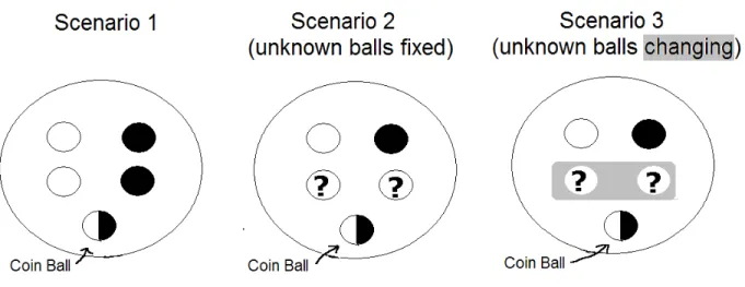
five balls that are either black or white. However, the scenarios differ in a way intended to illustrate alternative hypotheses about learning in economic environments, and to motivate the main ingredients of our model. Figure 1 illustrates the composition of the urns.

Scenario 1: Pure risk

An urn contains five balls. The agent is told that two are black, two are white and that the fifth is either black or white depending on the outcome of the toss of an unbiased coin - the ‘coin ball’ is black if the coin toss produces heads and it is white otherwise. She cannot see the outcome of the coin toss, but she does observe some possibly related signals, namely, in each period she sees a black or white ball. Suppose that she anticipates all this and that her ex ante view is that these data are generated by sampling with replacement from the given urn. This may be because she is actually doing the sampling, or because she has been told that this is how signals are generated. Alternatively, it may simply reflect her subjective view of the environment. In any case,

the obvious version of the Bayesian learning model (1) seems appropriate. In particular, she can be confident of learning the color of the coin ball.

It is useful to compare the preceding with the following alternative scenario (referred to later as Scenario10_{): signals are generated by successive sampling from a sequence of} urns, each containing black and white balls. Each urn is perceived as consisting of a coin ball and four other balls as above. The coin is tossed once at the start and determines the same color for coin-balls in all urns. However, non-coin balls are replaced every period with a new set of non-coin balls. Each set is determined by a new realization of an i.i.d. process that puts probability 1/2 each on 2 and 3 black non-coin balls.

At first sight, this scenario looks more complicated: the number of non-coin balls in any given urn is not known and cannot be learned because it changes over time. However, the fact that there is a known identical distribution over the number of black non-coin balls at all dates implies that Scenario 10 is effectively the same as Scenario 1: in both cases, the probability that a randomly drawn non-coin ball is black is 1/2 at all dates. This is all that matters for updating beliefs about what the next draw will be. Decisions that depend on the conditional probability of the next ball drawn, such as betting on the color of the latter, should thus be identical in the two scenarios. Similarly, in both cases beliefs about the total number of black balls in each urn will settle down at the long run empirical frequency of black draws.

The difference between the two alternative perceptions of signals - they are generated by sampling with replacement from a fixed urn on the one hand versus being due to sampling from different urns on the other - will play an important role below in the intuition for our model of learning under ambiguity. The fact that there is no meaningful difference between them here is a (restrictive) feature of the Bayesian model.

Scenario 2: Ambiguous priors and fixed urn

The information provided about the urn is modified to: there is at least one non-coin ball of each color. Thus unlike Scenario 1, no objective probabilities are given for the composition of the urn — there is ambiguity about the number of black non-coin balls. However, signals are again observed in each period and they are viewed as resulting from sampling with replacement from the given urn. Because the agent views the factors underlying signals, namely the color composition of the urn, as fixed through time, she can hope to learn it. That is, she would try to learn the trueθ _∈Θ=_{1₅,2₅,3₅,4_5}, where the connection to signals is expressed by the single likelihood

(B _|θ) =θ.

Compare this situation with the purely risky one, Scenario 1 above, assuming the two coin tosses are independent. In particular, consider the choice between betting on drawing black (white) from the risky urn as opposed to the ambiguous one. (Throughout abet on the color of a ball drawn from an urn is understood to pay one util if the ball has the desired color and zero otherwise.) The familiar Ellsberg Paradox examines this choice

Figure 1: Urns for Scenarios 1-3.

prior to any sampling. The intuitive behavior pointed to by Ellsberg is the preference to bet on drawing black from the risky urn as opposed to the ambiguous one, and a similar preference for white. This behavior is inconsistent with any single probability measure on the associated state space and hence also with any single prior on Θ. The intuition is that confidence about the odds differs across the two urns. This difference matters for behavior, but cannot be captured by probabilities. On the other hand, the multiple-priors model predicts the intuitive choices if the set _M0 of priors on Θ admits

the possibility that the number of black non-coin balls is less than 2 and similarly for white. Thus we are led to the triple (Θ,_M0, ), which differs from the Bayesian model only in that _M0 is a nonsingleton set.

Consider the ranking of bets after some sampling. Assuming that the agent’s prior view of signals is correct, actual learning proceeds in each case as though sampling is from an unchanging urn. Thus it is intuitive that for the ambiguous urn, learning should resolve ambiguity in the long run. As the number of draws increases, ambiguity should diminish and asymptotically the agent should behave as if she knew the fraction of black balls were equal to their empirical frequency - in the limit, and for any common sample history across the two urns, she would be indifferent between betting on the next draw from the risky as opposed to the ambiguous urn. Formally, increasing confidence about the ambiguous urn is captured in our model because the set _Mt of posteriors shrinks

with time.

Both Scenarios 1 and 2 are conducive to inference and learning because there is one urn withfixed composition. Next we examine learning in a more complex setting where signals are generated by a sequence of urns with time-varying composition. This added complexity was shown above to be of no consequence in the Bayesian model, but it will matter more generally.

Scenario 3: Unambiguous prior and changing urns

Signals are generated by successive sampling from asequence of urns, each containing black and white balls. The urns are perceived in the following way: each urn consists of a coin ball and four other balls as above. The coin is tossed once at the start and determines the same color for coin-balls in all urns. However, non-coin balls are replaced every period with a new set of non-coin balls. This task is performed every period by an administrator. It is also known that (i) a new administrator is appointed every period,

(ii) no administrator knows the previous history of urns or draws and (iii) the only restriction on any given administrator is that at least one non-coin ball of each color be placed in the urn.

Ex ante, before any draws are observed, this environment looks the same as Scenario 2: there is one coin ball, there is at least one black and one white non-coin ball, and there are two non-coin balls about which there is no information. The new feature in Scenario 3 is that the non-coin balls change over time in a way that is not well understood. What might an agent now try to learn? Since the coin-ball isfixed across urns and underlies all signals, it still makes sense to try to learn its color. At the same time, learning about the changing sequence of non-coin balls has become more difficult. Compared to Scenario 2, one would thus expect agents to perceive more uncertainty about the overall proportion of black balls. This leads to behavioral differences between the two scenarios in both the short and the long run.

Consider first betting behavior after a small number of draws, assuming that the coin tosses in Scenarios 2 and 3 are independent. Before any sampling, one should be indifferent between bets in Scenarios 2 and 3, since the two settings area priori identical. However, suppose that one black draw from each urn has been observed and consider bets on the next draw being black. It is intuitive that the agent prefer again to bet on the next urn in Scenario 2 because the black draw is stronger evidence there for the next draw also being black: in Scenario 3, the agent does not understand well the dynamics of the non-coin balls and thus is plausibly concerned that the next urn may contain more white balls than did the first. She thinks that it may also contain more black balls, but as in the static Ellsberg choice problem, the more pessimistic possibility outweighs the optimistic one. Thus she would rather bet in Scenario 2 where the number of black non-coin balls is perceived not to change between urns. Our model can accommodate this preference (see Section 4.1).

How does an agent expect to behave in the long run? A Bayesian might postulate a family of stochastic processes that describe the evolution of the non-coin balls over time. She would then hope to learn moments of that process, such as the fraction of black non-coin balls placed in the urn by the average administrator. However, any such approach makes sense only if the agent is confident that the fraction of black non-coin balls will converge to some limit. The description (or perception) of the environment provides no indication that this will happen. To the contrary, the ever-changing sequence of administrators suggests perpetual change.

inde-pendent across urns. Under this view, she does not expect to learn anything about future non-coin balls from sampling. Given how little information is provided about any single urn, it is then natural for her to perceive the number of non-coin balls as ambiguous at all dates. In particular, she expects that, after sufficiently long identical samples from the two scenarios, she will still prefer to bet on the next draw being black from the urns in Scenario 2 rather than in Scenario 3.

Multiple likelihoods to model changing urns

Our model of Scenario 3 builds on the Bayesian model in that it also starts from a parameter space — here Θ = _{B, W_}, corresponding to the two possible colors of the coin-ball — and a prior µ0, here the

¡₁

2, 1 2

¢

prior on Θ corresponding to the toss of the unbiased coin. In addition, ambiguity perceived about the changing non-coin balls motivates a set of likelihoods _L. The general idea is that of an agent who perceives the data generating mechanism as having some unknown features that are common across a set of experiments, represented by θ. At the same time, other unknown features are variable across experiments, represented by _L. It is known that the variable features are determined by a memoryless mechanism — this is why the set_L does not depend on history. It is also known that the relative importance of the variable features is the same every period, as in the urn example where there are always four non-coin balls and one coin ball. This is why the set_L does not depend on time.

In the urns example, the set of likelihoods might be specified as follows: letλ denote the number of black non-coin balls. Then the likelihood of drawing a black ball from that urn is given by

λ(B|θ) =

½ _λ+1

5 if θ =B

λ

5 if θ =W.

Given the symmetry of the environment, a natural set of likelihoods is

L =_{ λ :λ∈[2− ,2 + ]}, (2)

where is a parameter, 0_{≤ ≤}1.

In the special case = 1, the set _L models an agent who attaches equal weight to all logically possible urn compositions λ = 1, 2, or 3. More generally, (2) incorporates a subjective element into the specification. Just as subjective expected utility theory does not impose connections between the Bayesian prior and objective features of the environment, so too the set of likelihoods is subjective (varies with the agent) and is not uniquely determined by the facts. For example, the agent might attach more weight to the ‘focal’ likelihood corresponding to λ = 2 as opposed to the more extreme cases

λ = 1,3. The parameter can be interpreted as the weight attached to the latter cases, as opposed to the focal likelihood. Indeed, _L can be rewritten as7

L =_{(1₋ ) 2(· |θ) + λ(· |θ) : λ= 1, 2, 3}.

7_{This is a form of the -contamination model employed in robust statistics (see Walley [37], for}

We emphasize that the agent behaves as though she views any likelihood in _L as applying at any future time. In particular, she admits the possibility that the operative likelihood varies from period to period. Moreover, the way in which it can vary is con-strained only by the requirement that every likelihood lies in _L. This view is perfectly consistent with her limited information about the urns. The description of the environ-ment does not give any indication of patterns in the sequence of urns. In particular, past draws do not provide any information about the non-coin balls in future urns. The composition of the non-coin balls in the next urn is thusalways ambiguous, even after a large number of draws.8

It follows that Ellsberg-type choices in betting on the color of the next draw should persist forever, in contrast to what we have observed for Scenario 2. For example, after a sufficiently long sample, an agent will prefer to bet on the next draw being black from the urns in Scenario 2 rather than in Scenario 3. The model thus rationalizes a preference for bets in Scenario 2 over those in Scenario 3 in the long run. Section 4.1 below will show that it also captures the intuitive preference for bets in Scenario 2 in the short run. Updating

To motivate how we model behavior in the short run, turn to the agent’s view about

θ after afinite number of draws. Intuitively, the fraction of black draws observed in the past is informative about the parameter: the more black draws are observed, the more confident she should become that the coin ball is black. How quickly confidence will change now also depends on what she believes, with hindsight, about the sequence of non-coin balls in past urns. Importantly, while it is not possible to learn about future non-coin balls, past draws are certainly informative about past non-coin balls.9 _For

example, if a black ball was drawn two periods ago, it is more likely, with hindsight, that the urn from which draws were made at that date contain three black non-coin balls.

More generally, any view one might have about the past sequence of non-coin balls can be evaluated in light of a sample st = (s1, ..., st). In Scenario 3, such reevaluation

of the non-coin balls is important for updating about the parameter θ. To illustrate, suppose 50 draws have been observed, and 30 of them have been black. Given a theory about the non-coin balls, these observations suggest that the coin ball is more likely to be black than white. At the same time, given a value of the parameter, the observations suggest that more than half of the past urns contained three black non-coin balls. Sensible updating takes both of these features into account. Our approach is based on selecting theories about the data described by a prior and a sequence of likelihoods, and then taking conditionals of theories that explain the given sample well.

8_{Scenario 3 is thus similar to Scenario 1’ above in that the agent is a priori certain that she will never}

learn more about future non-coin balls than what she already knows a priori. The difference is that initial beliefs in Scenario 1’ are captured by a single probability measure for the non-coin balls, while in Scenario 3 the non-coin balls are viewed as ambiguous.

9_{In this respect, Scenario 3 again resembles Scenario 1’. In Scenario 1’, one can infer something about}

past realizations of the i.i.d. non-coin ball process from past draws. At the same time, the conditional distribution of future non-coin balls is always the same.

More specifically, consider the following heuristic reasoning. There is a large set of “theories” about sequences of data that the agent might be willing to entertain. Every theory is described by a probability measure on S∞ _{of the type}

Z

Π∞_j=1 j(.|θ)dµ0(θ), (3)

where µ_{0 ∈ M}0 is a prior and { t} ∈ L∞ is a sequence of likelihoods. Here every

theory says that the data are serially independent conditional on θ, but many allow for nonstationarity, although there are also theories that say the data are conditionally i.i.d. We define the agent’s set of one-step-ahead beliefs after a samplest_{as conditionals (given}

st_{) of probabilities of type (3). To capture reevaluation, we allow only conditionals of}

those probability measures that do a “good enough job” in explaining the sample st_,

which is formalized using an approriate likelihood ratio test. The stringency of the test becomes a parameterαthat governs how quickly agents are willing to resolve ambiguity.

3

A MODEL OF LEARNING

3.1

Recursive Multiple-Priors

We work with a finite period state space St = S, identical for all times. One element

st ∈S is observed every period. At timet, an agent’s information consists of the history

st _{= (s1, ..., s}

t). There is an infinite horizon, so S∞ is the full state space.10 The agent

ranks consumption plans c= (ct), where ct is a function of the history st. At any date

t = 0,1, ..., given the history st_{, the agent’s ordering is represented by a conditional}

utility functionUt, defined recursively by

Ut(c;st) = min p∈Pt(st)

Ep £u(ct) + βUt+1(c;st, st+1)

¤

, (4)

whereβandusatisfy the usual properties. The set of probability measures_Pt(st)models

beliefs about the next observationst+1, given the historyst.Such beliefs reflect ambiguity

when _Pt(st) is a nonsingleton. We refer to {Pt} as the process of conditional

one-step-ahead beliefs. The process of utility functions is determined by specification of_{Pt},u(·)

andβ, which constitute the primitives of the functional form.

To clarify the connection to the Gilboa-Schmeidler model, it is helpful to rewrite utility using discounted sums. In a Bayesian model, the set of all conditional-one-step-ahead probabilities uniquely determine a probability measure over the full state space. Similarly, the process _{Pt} determines a unique set of probability measures P on S∞

10_{In what follows, measures on S}∞ _{are understood to be defined on the product σ-algebra on S}∞_,

denoted by _S, and those on any St are understood to be defined on the power set of St. While our

formalism is expressed forSfinite, it can be justified also for suitable metric spacesS but we ignore the technical details needed to make the sequel rigorous more generally.

satisfying the regularity conditions specified in Epstein and Schneider [13].11 _{Thus one}

obtains the following equivalent and explicit formula for utility:

Ut(c;st) = min p∈P E p £_Σ s≥tβs−tu(cs) | st ¤ . (5)

This expression shows that each conditional ordering conforms to the multiple-priors model in Gilboa and Schmeidler [19], with the set of priors for time t determined by updating the set_P measure-by-measure via Bayes’ Rule.

Axiomatic foundations for recursive multiple-priors utility are provided in Epstein and Schneider [13]. The essential axioms are that(i)conditional orderings satisfy the Gilboa-Schmeidler axioms, and(ii)conditional orderings are connected by dynamic consistency. The analysis in [13] also clarifies the role of the set_P in an intertemporal multiple-priors model. In particular, _P should not be interpreted as the “set of time series models that the agent contemplates”. Indeed, the axioms imply restrictions on _P, although they do not impose structure on agents’ beliefs. Instead, restrictions on _P are needed to capture aspects of dynamic behavior, such as backward-induction reasoning implied by the dynamic consistency axiom. This observation is important for applications such as learning: if _P is selected on the basis of statistical criteria alone, this might have unintended, or hard-to-understand, consequences for dynamic behavior.

Recursive multiple priors has some important features in common with the standard expected utility model. Decision making after a historyst _{is not only dynamically}

consis-tent, but it also does not depend on unrealized parts of the decision tree. In other words, utility given the history st_{, depends only on consumption in states of the world that can}

still occur. To ensure such dynamic behavior in an application, it is sufficient to specify beliefs directly via a process of one-step-ahead conditionals_{Pt}.In the case of learning,

this approach has additional appeal. Because _{Pt}describes how an agent’s view of the

next state of the world depends on history, it is a natural vehicle for modeling learning dynamics. The analysis in [13] restricts_{Pt} only by technical regularity conditions. We

now proceed to add further restrictions to capture how the agent responds to data.

3.2

Learning

Our model of learning applies to situations where a decision-maker holds the a priori view that data are generated by the same memoryless mechanism every period. This a priori view also motivates the Bayesian model of learning about an underlying parameter from conditionally i.i.d. signals.

As in the Bayesian model outlined in the introduction, our starting point is again (a

finite period state spaceS and) a parameter spaceΘthat represents features of the data the decision-maker tries to learn. To accommodate ambiguity in initial beliefs about

11_{In the infinite horizon case, uniqueness obtains only if}

P is assumed also to be regular in a sense defined in Epstein and Schneider [14], generalizing to sets of priors the standard notion of regularity for a single prior.

parameters, represent those beliefs by a set _M0 of probability measures on Θ. The

size of _M0 reflects the decision-maker’s (lack of) confidence in the prior information on

which initial beliefs are based. A technically convenient assumption is that_M0 is weakly

compact;12 _{this permits us to refer to minima, rather than infima, over}

M0.

Finally, we adopt a set of likelihoods _L - every parameter value θ _∈ Θ is associated with a set of probability measures

L(_{· |}θ) = _{ (_{· |}θ) : _∈L}.

Each : Θ _−→ ∆(S) is a likelihood function, so that θ _7−→ (A _| θ) is assumed measurable for everyA_⊂S. Another convenient technical condition is that_Lis compact when viewed as a subset of(∆(S))Θ (under the product topology). Finally, to avoid the problem of conditioning on zero probability events, assume that each (_{· |}θ) has full support.

Turn to interpretation. If there is a single likelihood, that is _L=_{{ }}, then any given

θ determines a unique probability measure onS∞. More generally, a nonsingleton set of likelihoods reflects the decision-maker’s view that θ alone does not uniquely determine the data generating mechanism. She feels there are other factors underlying data and this will influence her beliefs and preference. Beliefs about the signalstare described by

the same set_L for everyt — this captures the perception that the same mechanism is at work every period. Moreover, for a given parameter value θ _∈ Θ, signals are assumed to be independent over time — the mechanism is perceived to be memoryless. Factors modeled byθ are perceived as common across time or experiments - thus the agent can try to learn about them. Those modeled by the set _L are variable across time in a way that she does not understand beyond the limitation imposed by_L. In particular, at any point in time, any element of _L might be relevant for generating the next observation. Accordingly, while she can try to learn the true θ, she has decided that she will not try to (or is not able to) learn more.

Conditional independence implies that past signals st _{affect beliefs about future}

sig-nals (such as st+1) only to the extent that they affect beliefs about the parameter. Let

Mt(st), to be described below, denote the set of posterior beliefs aboutθ given that the

sample st _{has been observed. The dynamics of learning can again be summarized by a}

process of one-step-ahead conditional beliefs. However, in contrast to the Bayesian case (1), there is now a (typically nondegenerate)set assigned to every history:

Pt(st) = ½ pt(·) = Z Θ (_{· |}θ)dµ_t(θ) :µ_t∈Mt(st), ∈L ¾ , (6)

or, in convenient notation,

Pt(st) =

Z Θ L

(_{· |}θ)d_Mt(θ).

12_{More precisely, measures inM}

0 are defined on the implicit and suppressedσ-algebraB associated

with Θ. Take the latter to be the power set whenΘ is finite. The weak topology is that induced by bounded and_B-measurable real-valued functions on Θ. _M0 is weakly compact iffit is weakly closed.

This process enters the specification of recursive multiple priors preferences (4).13

Updating and reevaluation

To complete the description of the model, it remains to describe the evolution of the posterior beliefs _Mt. Imagine a decision-maker at time t looking back at the sample

st. In general, she views both her prior information and the sequence of signals as ambiguous. As a result, she will typically entertain a number of different theories about how the sample was generated. Adapting the notation used in the Bayesian case above, a theory is now summarized by a pair (µ0, t), where t = ( 1, .., t) ∈ Lt is a sequence

of likelihoods. The decision-maker contemplates different sequences t_{because she is not}

confident that signals are identically distributed over time.

We allow for different attitude towards past and future ambiguous signals. On the one hand, _L is the set of likelihoods possible in the future. Since the decision-maker has decided she cannot learn the true sequence of likelihoods, it is natural that beliefs about the future must be based on the whole set_L as in (6). On the other hand, the decision-maker mayreevaluate, with hindsight, her views about what sequence of likelihoods was relevant for generating datain the past. Such revision is possible because the agent learns more about θ and this might make certain theories more or less plausible. For example, some interpretation of the signals, reflected in a certain sequence t_{= ( 1, ...,}

t), or some

prior experience, reflected in a certain prior µ0 ∈M0, might appear not very relevant if

it is part of a theory that does not explain the data well.

To formalize reevaluation, we need two preliminary steps. First, how well a theory

(µ₀, t_{)explains the data is captured by the (unconditional) data density evaluated at s}t_:

Z

Πtj=1 j(sj|θ)dµ0(θ).

Here conditional independence implies that the conditional distribution givenθ is simply the product of the likelihoods j. Prior information is taken into account by integrating

out the parameter using the prior µ₀. The higher the data density, the better is the observed sample st _{explained by the theory (µ}

0, t). Second, let µt(· ;st, µ0, t) denote

the posterior derived from the theory (µ0, t) by Bayes’ Rule given the data st. This

posterior can be calculated recursively by Bayes’ Rule, taking into account time variation in likelihoods: dµt ¡ · ;st, µ0, t ¢ = R t(st | ·) Θ t(st|θ 0_)dµ t−1(θ0;st−1, µ0, t−1) dµt−1(· ;st, µ0, t−1). (7)

Reevaluation takes the form of a likelihood-ratio test. The decision-maker discards all theories (µ0, t) that do not pass a likelihood-ratio test against an alternative theory

13_{Given compactness of M}

0 and L, one can show that Mt(st) defined below is also compact, and

that puts maximum likelihood on the sample. Posteriors are formed only for theories that pass the test. Thus posteriors are given by

Mαt(s t_{) =} {µ_t¡st;µ₀, t¢: µ_{0 ∈M}, t_∈Lt, (8) Z Πt_j=1 j(sj|θ)dµ0(θ)≥α max ˜ µ₀∈M0 ˜t_∈Lt Z Πt_j=1˜j(sj|θ)dµ˜0}.

Here α is a parameter, 0< α_≤ 1, that governs the extent to which the decision-maker is willing to reevaluate her views about how past data were generated in the light of new sample information. The likelihood-ratio test is more stringent and the set of posteriors smaller, the greater is α. In the extreme case α = 1, only parameters that achieve the maximum likelihood are permitted. If the maximum likelihood estimator is unique, ambiguity about parameters is resolved as soon as the first signal is observed. More generally, we have that α > α0 _{implies M}α

t ⊂ Mα

0

t . It is important that the test is

done after every history. In particular, a theory that was disregarded at time t might look more plausible at a later time and posteriors based on it may again be taken into account.

In summary, our model of learning about an ambiguous memoryless mechanism is given by the tuple (Θ,_M0,_L, α). As described, the latter induces, or represents, the process _{Pt} of one-step-ahead conditionals via

Pt(st) =

Z Θ L

(_{· |}θ)d_Mαt(θ),

where _Mα

t is given by (8). The model reduces to the Bayesian model when both the set

of priors and the set of likelihoods have only a single element.

Another important special case occurs if _M0 consists of several Dirac measures on

the parameter space in which case there is a simple interpretation of the updating rule: Mα

t contains all ˜θ’s such that the hypothesis θ = ˜θ is not rejected by an asymptotic

likelihood ratio test performed with the given sample, where the critical value of the

χ2_{(1)distribution is}

−2 log α. Sinceα > 0, (Dirac measures over) parameter values are discarded or added to the set, and _Pt varies over time. The Dirac priors specification is

convenient for applications — it will be used in our portfolio choice example below. Indeed, one may wonder whether there is a need for non-Dirac priors at all. However, more general priors provide a useful way to incorporate objective probabilities, as illustrated by the scenarios in Section 2.14

4

PROPERTIES

In this section we illustrate properties of learning under ambiguity in the context of the scenarios described above. We show that our model rationalizes the intuitive choices

14_{Another example is in Epstein and Schneider [15], where a representation with a single prior and}

α= 0 is used to model the distinction between tangible (well-measured, probabilistic) and intangible (ambiguous) information.

described in Section 2, and we examine the dynamics of beliefs and confidence in the short term. Then we provide a result on convergence of the learning process in the long run.

4.1

Scenarios Revisited

We described in Section 2 how we would model the three scenarios. The intuitive Ellsberg-type behavior would obviously be captured in this way. Focus on the other choice de-scribed above - given that one black ball has been drawn, would you rather bet on the next draw being black in Scenario 2 or in Scenario 3? This question highlights one difference between learning in simple settings (Scenario 2) as opposed to complex ones (Scenario 3), and correspondingly demonstrates the key role played by multiple-likelihoods. We argued above that it is intuitive that one prefer to bet in Scenario 2 - the black draw is stronger evidence there for the next draw also being black. We now propose a natural specification of beliefs for both Scenarios for which these choices obtain.

Scenario 2: To define a representation(Θ,_M0,_L, α), take Θ=©n₅ : n= 1,2,3,4ª, the proportion of black balls (coin or non-coin), and (B _|θ) = θ. Specify the set _M0 of

priors onΘas follows: the true overall proportion isθ iffthere are5θ black balls in total. Let

P _⊂∆(_{1,2,3_})

denote beliefs about the number of black non-coin balls. Since the coin-ball and other colors are independent, each prior µ0 should have the form

µp₀(θ) = 1₂p(5θ₋1) + 1₂p(5θ) (9) for some p_∈P. Thus

M0 ={µ

p

0 : p∈P}.

Finally, fix a reevaluation parameterα.

Scenario 3: Take Θ=_{B, W_}, corresponding to the two possible colors of the coin ball,

µ₀ =¡1₂,1₂¢, and define likelihoods as follows: letP _⊂∆(_{1,2,3_}) denote beliefs about number of black non-coin balls, where P is the same set used in Scenario 2. Since the

first urns in the two scenarios are identical, it is natural to use the same setP to describe beliefs about them. Moreover, though the urns differ along the sequence in Scenario 3, successive urns are indistinguishable, which explains whyP can be used also to describe the second urn in the present scenario. Eachp inP suggests one likelihood function via

p_(B |B) = Σλ p(λ) + 1 5 , p_(B |W) = Σλ p(λ) 5 , and15 L=_{ p : p_∈P_}.

15_{If P = {p∈∆({1,2,3}) : Σλp(λ) ∈ [2− ,2 + ]}, for given , then the corresponding set of}

The appendix shows that the intuitive choices discussed in Section 2 follow from these beliefs. In particular, it demonstrates that the minimal predictive probability for a black ball conditional on observing a black ball,

min p P1(B) = _∈L,µmin₁∈Mα 1(B) Z Θ (B _|θ)dµ₁(θ),

is smaller under Scenario 3 than under Scenario 3. An ambiguity averse agent who ranks bets according to the smallest probability of winning will thus prefer to bet on the urn from Scenario 2.

4.2

Inference from Small Samples

We use Scenario 3 here to illustrate the short run dynamics of beliefs (and confidence) that can be delivered by our model. Once again, take Θ = _{B, W_}, µ0 =

¡₁ 2, 1 2 ¢ , and for the set of likelihoods take _L from (2) with = 1 - the agent weighs equally all the logically possible combinations of non-coin balls. The evolution of the posterior set Mαt in (8) shows how signals tend to induce ambiguity about parameters even where

there is no ambiguity ex ante (singleton_Mα

0). This happens when the agent views some

aspects of the data generating mechanism as too difficult to try to learn, as modeled by a nonsingleton set of likelihoods. More generally, _Mαt can expand or shrink depending

on the signal realization.

Posterior beliefs can be represented by the intervals

[ min

µt∈Mαt

µ_t(B), max

µt∈Mαt

µ_t(B)].

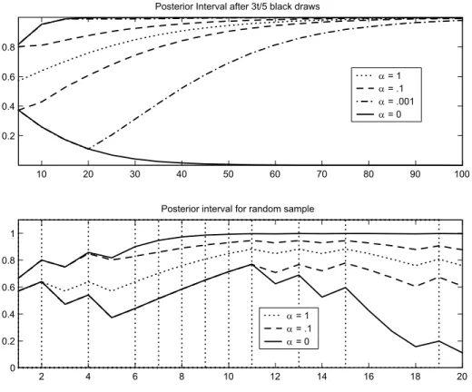
Figure 2 depicts the evolution of beliefs about coin-ball being black as more balls are drawn. The top panel shows the evolution of the posterior interval for a sequence of draws such that the number of black balls is 3₅t, for t = 5,10, .... Intervals are shown for

α = .1 and α = .001, as well as for α = 0, to illustrate what would happen without revaluation. In addition, a single line is drawn for the case α = 1, where the interval is degenerate. For example, after the first 5 signals, with 3 black balls drawn, the agent withα=.1assigns a posterior probability between.4and.8to the coin ball being black. What happens if the same sample is observed again? There are two effects. First, a larger batch of signals permits more possible interpretations of past signals. For example, having seen ten draws, the agent may believe that all six black draws came aboutalthough each time there were the most adverse conditions, that is, all but one non-coin ball was white. This interpretation strongly suggests that the coin ball itself is black. The argument also becomes stronger the more data are available - after only five draws, the appearance of three black balls under ‘adverse conditions’ is not as remarkable. At the same time, the story that all but one non-coin ball was always white is somewhat less believable if the sample is larger: reevaluation limits the scope for interpretation, and more so the more data are available. The evolution of confidence, measured by the size of the posterior interval, thus depends on how much agents reevaluate their views. For

10 20 30 40 50 60 70 80 90 100 0.2

0.4 0.6 0.8

Posterior Interval after 3t/5 black draws

α = 1 α = .1 α = .001 α = 0 2 4 6 8 10 12 14 16 18 20 0 0.2 0.4 0.6 0.8 1

Posterior interval for random sample

α = 1

α = .1

α = 0

Figure 2: The Posterior Interval is the range of posterior probability that the coin ball is black, µt(B). In the top panel, the sample is selected to keep fraction of black balls

constant. In the bottom panel, vertical lines indicate black balls drawn.

an agent with α = .001, the posterior interval expands between t = 5 and t = 20. In this sense, a sample of ten or twenty ambiguous signals induces more ambiguity than a sample of five. However, reevaluation implies that large enough batches of ambiguous signals induce less ambiguity than smaller ones.

The lower panel of Figure 2 tracks the evolution of posterior intervals along one particular sample. Black balls were drawn at dates indicated by vertical lines, while white balls were drawn at the other dates. Taking the width of the interval as a measure, the extent of ambiguity is seen to respond to data. In particular, a phase of many black draws (periods 5-11, for example) shrinks the posterior interval, while an ‘outlier’ (the white ball drawn in period 12) makes it expand again. This behavior is reminiscent of the evolution of the Bayesian posterior variance, which is also maximal if the fraction of black balls is one half.

4.3

Beliefs in the Long Run

Turn now to behavior after a large number of draws. As discussed above, our model describes agents who are not sure whether empirical frequencies will converge.

Neverthe-less, it is useful to derive limiting beliefs for the case when such convergence occurs: the limiting beliefs also approximately describe behavior after a large, but finite, number of draws. Therefore, they characterize behavior in the long run. The limiting result below holds with probability one under a true data-generating process, described by a prob-ability P∗ _{on (S}∞_{,S). For this process, we require only that the empirical frequencies}

of each of the finite number of states s _∈ S converge, almost surely under P∗_{. In what}

follows, these limiting frequencies are described by a measure φ on S.

By analogy with the Bayesian case, the natural candidate parameter value on which posteriors might become concentrated maximizes the data density of an infinite sample. With multiple likelihoods, any data density depends on the sequence of likelihoods that is used. In what follows, it is sufficient to focus on sequences such that the same likelihood is used whenever state s is realized. A likelihood sequence can then be represented by a collection ( s)_s∈S. Accordingly, define the log data density after maximization over the

likelihood sequence by H(θ) := max ( s)s∈S X s∈S φ(s) log s(s|θ). (10)

The following result (proven in the appendix) summarizes the behavior of the posterior set in the long run.

Theorem 1 Suppose that Θ is finite and that:

(i) θ∗ = arg maxθH(θ) is a singleton;

(ii) there exists κ such that for every µ0 in Mα0,

either µ₀(θ∗) = 0 orµ₀(θ∗)_≥κ, and µ0(θ∗)>0 for some µ0 inMα0.

Then every sequence of posteriors from _Mα

t converges to the Dirac measure δθ∗, almost

surely under the true probability P∗_{, and the convergence is uniform, that is, there is a}

set Ω_⊂S∞ with P∗(Ω) = 1 and such that for every s∞ in Ω,

µ_t(θ∗)_→1

uniformly over all sequences of posteriors _{µt} satisfying µt ∈Mαt (st) for all t.

Condition (i)is an identification condition: it says that there is at least one sequence of likelihoods (that is, the maximum likelihood sequence), such that the sample with empirical frequency measure φ can be used to distinguishθ∗ from any other parameter value. Condition (ii) is satisfied if every prior in_Mα

0 assigns positive probability to θ∗

(because _Mα

0 is weakly compact). The weaker condition stated accommodates also the

case where all priors are Dirac measures (including specifically the Dirac concentrated at θ∗), as well as the case of a single prior containingθ∗ in its support. (In Scenario 3,

(ii)is satisfied for any set of priors where the probability of a black coin ball is bounded away from zero.)

Under conditions(i)and(ii), and ifΘisfinite, then in the long run only the maximum likelihood sequence is permissible and the set of posteriors converges to a singleton. The agent thus resolves any ambiguity about factors that affect all signals, captured byθ. At the same time, ambiguity about future realizations st does not vanish. Instead, beliefs

in the long run become close to _L(_·|θ∗). The learning process settles down in a state of time-invariant ambiguity.

The asserted uniform convergence is important in order that convergence of beliefs translate into long-run properties of preference. Thus it implies that for the process of one-step-ahead conditionals _{Pt} given by (6),

Pt(st) = Z Θ L (_{· |}θ)d_Mαt(θ), we have min pt∈Pt Z f(st+1)dpt= min µ_t∈Mα t min ∈L Z Θ ·Z St+1 f(st+1)d (st+1 |θ) ¸ dµt(θ) →min ∈L Z St+1 f(st+1)d (st+1 |θ∗),

for any f : St+1 → R1 describing a one-step-ahead prospect (in utility units). In

par-ticular, this translates directly into the utility of consumption processes for which all uncertainty is resolved next period.

Long run behavior in Scenario 3

As a concrete example, consider long run beliefs about the urns in Scenario 3. Letφ_∞

denote the limiting frequency of black balls. Suppose also that beliefs are given by (2) with = 1. Maximizing the data density with respect to the likelihood sequence yields

H(θ) =φ_∞max λB log1{θ=B} +λB 5 + (1−φ∞) maxλW log5−1{θ=B}−λW 5 =φ_∞log1{θ=B}+ 3 5 + (1−φ∞) log 4₋1_{θ=B} 5 .

The first term captures all observed black balls and is therefore maximized by assuming

λB = 3 black non-coin balls. Similarly, the likelihood of white draws is maximized by

settingλW = 1.It follows that the identification condition is satisfied except in the

knife-edge case φ_∞ = 1₂. Moreover, θ∗ = B if and only if φ_∞ > 1₂. Thus the theorem implies that an agent who observes a large number of draws with a fraction of black balls above one half believes it very likely that the color of the coin ball is black. The role of α is only to regulate the speed of convergence to this limit. This dependence is also apparent from the dynamics of the posterior intervals in Figure 2.

The example also illustrates the role of the likelihood ratio test (8) in ensuring learn-ability of the representation. Suppose that φ_∞ = 3₅. The limiting frequency of 3₅ black draws could be realized either because there is a black coin ball and on average one half of the non-coin balls were black, or because the coin ball is white and all of the urns contained 3 black non-coin balls. If α were equal to zero, both possibilities would be taken equally seriously and the limiting posterior set would contain Dirac measures that place probability one on either θ = B or θ = W. This pattern is apparent from Figure 2. In contrast, with α > 0, reevaluation eliminates the sequence where all urns contain three black non-coin balls as unlikely.16

Memoryless truths

The set of “true” processes P∗ for which the theorem holds is large. Like a Bayesian who is sure the data are exchangeable, the agent described by the theorem is convinced that the data generating process is memoryless. As a result, learning is driven only by the empirical frequencies of the one-dimensional events, or subsets of S. Given any process for which those frequencies converge to a given limit, the agent will behave in the same way. For example, if the data were generated by a stationary Markov chain, the agent would not react to the resulting patterns of serial dependence, and act the same way as if the data were serially independent. Of course, in applications one would typically consider a “truth” that is memoryless. Like the exchangeable Bayesian model, our model is best applied to situations where the agent iscorrect in his a priori judgement that the data generating process is memoryless.

Importantly, a memoryless process for which empirical frequencies converge need not be i.i.d. There exists a large class of serially independent, but nonstationary, processes for which empirical frequencies converge. In fact, there is a large class of such processes that cannot be distinguished from an i.i.d. process with distributionφon the basis of any

finite sample. A concern with ongoing change may thus lead agents to never be confident that they have identified a “true” i.i.d. data generating process with distributionφ, even if they are convinced that the empirical frequencies converge.17

For a simple example, consider two measuresφ1 and φ0 on S such thatφ is a convex

combination, that is, there is a number ω _∈(0,1)such that φ =ωφ1+ (1−ω)φ0. Now

let ω˜t be an i.i.d. process valued in {0,1} with Pr (˜ωt = 1) = ω. To construct a new

nonstationary process on the state spaceS, first fix a realizationω = (ωt) of the process

(˜ωt).Then consider the serially independent process (sωt) where the distribution ofsωt is

φ_t =ωtφ1+ (1−ωt)φ0.For almost every realization ω, the empirical distribution of the

nonstationary process(sω

t)will now converge to that of an i.i.d process with distribution

φ.18 Without further information, agents who have observed a lot of i.i.d. data with

16_{With a stronger identification condition, then even if α = 0, the posterior set converges to the}

singleton set consisting of the Dirac measure concentrated on θ∗. This case is discussed further in Epstein and Schneider [15].

17_{As discussed earlier, they may also reach this view because they are not sure whether the empirical}

frequencies converge in thefirst place.

distribution φ cannot rule out the possibility that the true data generating process is nonstationary — it could be any of the nonstationary processes indexed by a typical realizations ω. Moreover, since ωt+1 is unknown for any finite t, agents may not be sure

that the distribution of the next realization is φ — for all they know, it might be φ₀ or

φ₁. Non-vanishing ambiguity is one way to capture this concern with ongoing change.

5

DYNAMIC PORTFOLIO CHOICE

Selective asset market participation is puzzling in light of standard models based on expected utility and rational expectations. In contrast, it is consistent with optimalstatic portfolio choice by investors who are averse to ambiguity in stock returns. Such investors will take a nonzero (positive or negative) position in an asset only if it unambiguously promises an expected gain. Dow and Werlang [11] consider an investor who allocates wealth between a riskless asset and one other asset with ambiguous return. They show that if the range of premia on the ambiguous asset contains zero, it is optimal to invest 100% in the riskless asset. The intuition is that, when the range of premia contains zero, the worst case expected excess return on both long and short positions is not positive.

In practice, most investors do not make one-shot portfolio choices, but have long investment horizons during which they repeatedly rebalance their portfolios. Here we consider an intertemporal problem, where the investor updates his beliefs about future returns. For simplicity, we follow Dow and Werlang by restricting attention to the case of a single uncertain asset. However, the effects we emphasize are relevant more widely. Indeed, work by Epstein and Wang [16] and Mukherji and Tallon [31] has clarified that the basic nonparticipation result extends toselective participation when many assets are available. The key observation is that the multiple-priors model allows confidence to vary across different sources of uncertainty.19 Investors will participate in a market only if they are confident that they know how to make money in that particular market. 20

Suppose the investor cares about wealth T periods from now and plans to rebalance his portfolio once every period. There is a riskless asset with constant gross interest rate Rf_{, as well as an asset with uncertain gross return R}˜

t = R(st) that depends on

the historyst observed by the investor. Signals may consist of more than current excess returns. Beliefs are given by a process of one-step-ahead conditionals _{Pt}. At date t,

given information st_{, the investor selects a portfolio weight ω(s}t_{) for the risky asset by}

19_{For example, suppose that the set of excess return distributions for each available asset contains a}

component with unknown mean that is uncorrelated with the return on other assets. The range of mean excess returns for a particular asset now reflects investor confidence towards that asset only. If the range is a large interval around zero, that is, investor confidence is low, it is optimal to allocate zero wealth to the asset.

20_{This intuitionfits well with evidence from surveys among practitioners, who participate in a market}

only if they “have a view” about price movements of the asset in question. See Chew [9, Ch. 43] for a discussion of this issue.

solving the recursive problem Vt ¡ Wt, st ¢ = max ω pt∈minPt(st) Ept£_V t+1 ¡ Wt+1, st+1 ¢¤ subject to Wt = ¡ Rf + (R¡st¢₋Rf)ω¡st−1¢¢Wt−1, t= 1, ..., T. (11)

This problem differs from existing work on portfolio choice with multiple-priors be-cause beliefs are time-varying. We also emphasize the role of the investor’s planning horizon T. In Section 5.1, we discuss the nature of intertemporal hedging with recur-sive multiple-priors. To distinguish intertemporal hedging due to time-varying ambiguity from the intertemporal substitution effects stressed by Merton [30], we focus on the case of log utility, where traditional hedging demand is zero. In Section 5.2, we study a cal-ibrated example of asset allocation between stocks and riskless bonds for U.S. investors in the post-war period.

5.1

Intertemporal Hedging and Participation

If future investment opportunities and future returns are affected by common unknown (ambiguous) factors, then investors who have a longer planning horizon, and therefore care about future investment opportunities, will deal differently with ambiguity than short term investors. For example, if expected returns in some market are perceived to be highly ambiguous, the optimal myopic policy may be non-participation, to avoid exposure to ambiguity. However, if returns are also a signal of future expected returns, then a long-horizon investor is already exposed to the unknown (ambiguous) factor that is present in returns even if she does not currently participate in the market. It may then be better to take a position to offset existing exposure. We now derive intertemporal hedging demand due to ambiguity for the log utility case. We then discuss how the importance of hedging depends on the structure of ambiguity, and what this implies for the emergence of dynamic participation rules.

Hedging ambiguity

In the expected utility case, it is well known that log investors act myopically; even if the conditional distribution of future investment opportunities changes over time, the income and substitution effects of these changes are exactly offsetting. As a result, the investor’s asset demand depends only on current investment opportunities, captured by the conditional one-period-ahead distribution of returns. The optimal weight after history

st _{and given the beliefs process}

{pt} is simply ω∗¡pt ¡ st¢¢:= arg max ω E pt(st)h_log³_Rf ₊³_R˜ t+1−Rf ´ ω´i.

historyst, such an agent solves max ω pt(smint)∈P(st) Ept(st) h log ³ Rf + ³ ˜ Rt+1−Rf ´ ω ´i = min pt(st)∈P(st) Ept(st)h_log³_Rf ₊³_R˜ t+1−Rf ´ ω∗¡pt ¡ st¢¢´i, (12) where we have used the minmax theorem to exchange the order of optimization. Denote by pmyopict (st) the minimizing (conditional-one-step-ahead) measure in (12). Then the

optimal policy of a myopic agent isω∗¡_pmyopic t (st)

¢

, the portfolio weights that are optimal for the corresponding Bayesian.

For the intertemporal problem (11), conjecture the value functions Vt(Wt, st) =

logWt +ht(st), with hT = 0. Again using the minmax theorem, as well as the

bud-get constraint, we obtain

Vt ¡ Wt, st ¢ = min pt(st)∈Pt(st) max ω E pt£_V t+1 ¡ Wt+1, st+1 ¢¤ = min pt(st)∈Pt(st) n max ω E pt h log³Rf +³R˜t+1−Rf ´ ω´i+Ept£_h t+1 ¡ st+1¢¤o + logWt.

The first term depends only on time and st_{, verifying the conjecture for V}

t. Denote by p∗ t(st) a minimizing measure in ht ¡ st¢= min pt∈Pt(st) Ept h log³Rf +³R˜t+1−Rf ´ ω¡pt ¡ st¢¢´+ht+1 ¡ st+1¢i. (13) Then ω∗_(p∗

t(st))is an optimal policy for the intertemporal problem.

Comparison of (12) and (13) reveals that the supporting probabilities pmyopict andp∗t,

and hence the optimal policies in the myopic and intertemporal problems, need not agree. This motivates a decomposition of optimal portfolio demand ωt in the intert