SFED: A Rate Control Based Active Queue
Management Discipline
Abhinav Kamra, Sundeep Kapila, Varun Khurana, Vikas Yadav, Rajeev Shorey, Huzur Saran & Sandeep Juneja.
IBM India Research Laboratory, New Delhi, India Block 1, Indian Institute of Technology,
Hauz Khas, New Delhi 110016, India. Phone: 91-11-6861100; Fax: 91-11-6861555.
Abstract
Active queue management disciplines such as RED and its extensions (CHOKe, FRED, BRED) have been widely studied as mechanisms for providing congestion avoidance, differentiated services and fairness between different traffic classes. With the emergence of new applications with diverse QoS requirements over the Internet, the need for mechanisms that provide differentiated services has become increasingly important. We propose Selective Fair Early Detection (SFED), a rate control based queue management discipline which ensures a fair bandwidth allocation amongst competing flows even in the presence of non-adaptive traffic. We show that SFED can be used to partition bandwidth in proportion to pre-assigned weights and is well-suited for allocation of bandwidth to aggregate flows as required in the differentiated services framework. We study and compare SFED with other well known queue management disciplines and show that SFED ensures fair allocation of bandwidth across a much wider range of buffer sizes at a bottleneck router. We then propose a more efficient version of SFED using randomization that has an O(1) average time complexity, and, is therefore scalable.
Keywords
Internet, Router, Adaptive flows, Non-Adaptive flows, Congestion avoidance, Bandwidth, Fairness, TCP, UDP, Differentiated services
I. INTRODUCTION
Adaptive protocols such as the Transmission Control Protocol (TCP) employ end-to-end congestion con-trol algorithms [10]. These protocols adjust their sending rate on indications of congestion from the network in the form of dropped or marked packets [8]. However, the presence of non-adaptive flows in the Internet, gives rise to issues of unfairness. Adaptive flows back off by reducing their sending rate upon detecting congestion while non-adaptive flows continue to inject packets into the network at the same rate. Whenever adaptive and non-adaptive flows compete, the non-adaptive flows because of their aggressive nature, grab a larger share of bandwidth, thereby depriving the adaptive flows of their fair share. This gives rise to the need for active queue management disciplines [6] at intermediate gateways which provide protection for adaptive traffic from aggressive sources that try to consume more than their “fair” share, ensure “fairness” in bandwidth sharing and provide early congestion notification.
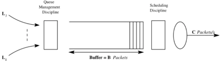
With the emergence of newer applications, each having its own resource requirements, it has become necessary to deploy algorithms at intermediate gateways that provide differentiated services [17] to the various types of traffic. Often flows of similar nature form one aggregate so that all flows within an aggregate receive the same QoS. Clark [16] suggests a model for differential bandwidth allocation between classes of flows. Flows within an aggregate can have further classifications resulting in a hierarchy [15] of flows. Efficient mechanisms to implement such classifications at intermediate gateways are of considerable interest. Figure 1 shows a typical Internet gateway with multiple incoming links, a single outgoing link of band-width C packets/s and a buffer size of B packets. The queue management discipline, operating at the
en-Dr. R. Shorey is with IBM India Research Laboratory, India.
Dr. Huzur Saran is with the Department of Computer Science and Engineering, Indian Institute of Technology, New Delhi, India. Dr. Sandeep Juneja is with the Department of Mechanical Engineering, Indian Institute of Technology, New Delhi, India.
1 L Lk Scheduling Discipline Queue Management Discipline C Packets/s Buffer = B Packets
Fig. 1. A typical Internet gateway
queuing end, determines which packets are to be enqueued in the buffer and which are to be dropped. The scheduling discipline, at the dequeuing end, determines the order in which packets in the buffer are to be dequeued. Sophisticated scheduling algorithms, such as WFQ, can be used to provide differentiated services to the various types of traffic. However, for early detection and notification of congestion a queue manage-ment discipline is necessary. Combinations of queue managemanage-ment and scheduling disciplines can provide early congestion detection and notification and can be used in the differentiated services framework. Com-plex scheduling mechanisms such as WFQ require per flow queues and as such have high implementation overheads.
In this paper we present Selective Fair Early Detection (SFED), a queue management discipline which when coupled with even the simplest scheduling discipline, such as First Come First Served (FCFS), achieves the following goals:
(i) Fair bandwidth allocation amongst flows, aggregates of flows and hierarchy.
(ii) Congestion avoidance by early detection and notification.
(iii) Low implementation complexity.
(iv) Easy extension to provide differentiated services.
SFED is a queue management algorithm to deal with both adaptive and non-adaptive traffic while providing incentive for flows to incorporate end-to-end congestion control. It uses a rate control based mechanism to achieve fairness amongst flows. As in Random Early Detection (RED) [1], congestion is detected early and notified to the source. SFED is easy to implement in hardware and is optimized to give
complexity for both enqueue and dequeue operations. We compare SFED with other queue management schemes such as RED, CHOKe [3], Flow Random Early Drop (FRED) [2], and observe that SFED performs at least as well as FRED and significantly better than RED and CHOKe. However, when buffer sizes are constrained, it performs significantly better than FRED.
We also demonstrate that SFED performs well when (i) flows are assigned different weights, (ii) when used to allocate bandwidth between classes of traffic such as would be required in the differentiated services scenario, and (iii) when it is used for hierarchical sharing of bandwidth.
The paper is organized as follows. In Section II, we briefly describe the existing queue management policies. An overview of SFED is presented in Section III. We describe our basic mechanism and how it is used to achieve the desired properties of a queue management discipline. Section IV explains our proposed algorithm in detail. We show how using randomization, our proposed algorithm can be optimized to give
performance. We then describe its hardware implementation. We compare the performance of SFED with other gateway algorithms namely RED, CHOKe and FRED with the help of simulations conducted using the ns2 [9] network simulator in Section V. In Section VI, we show how SFED can be generalized for weighted, aggregate and hierarchical flows. We summarize our results in Section VII. In the Appendix, we build an analytical model for SFED and demonstrate that fair sharing of bandwidth amongst flows can be achieved. We also discuss the effect of buffer size and round trip time on fairness achieved by SFED.
II. RELATEDWORK
A number of approaches for queue management at Internet gateways have been studied earlier. RED [1] addresses some of the drawbacks of droptail gateways. An RED gateway drops incoming packets with a dynamically computed probability when the exponential weighted moving average queue size exceeds
a threshold called . This probability increases linearly with increasing till after which
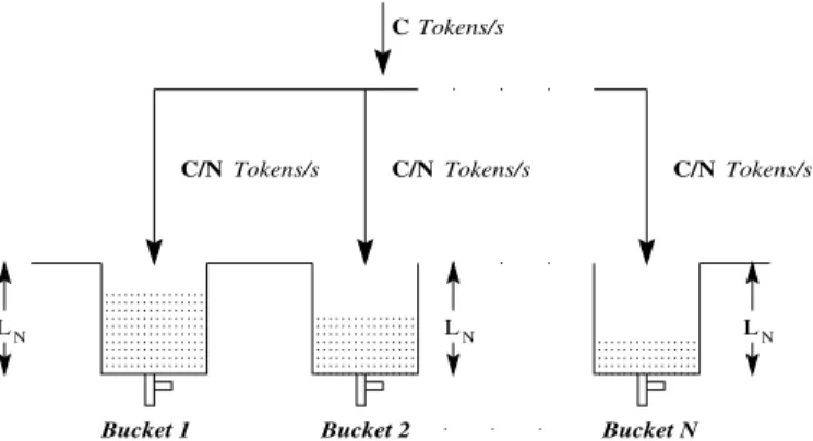
LN LN LN CTokens/s Bucket 1 Bucket 2 Tokens/s Tokens/s Tokens/s C/N C/N C/N Bucket N
Fig. 2. SFED architecture for rate control using token buckets
on the number of packets enqueued since the last packet drop. The goal of RED is to drop packets from each flow in proportion to the amount of bandwidth it is using. However, from each connection’s point of view the packet loss rate during a short period is independent of the bandwidth usage as shown in [2]. This contributes to unfair link sharing in the following ways:
Even a low bandwidth TCP connection observes packet loss which prevents it from using its fair share
of bandwidth.
A non-adaptive flow can increase the drop probability of all the other flows by sending at a fast rate.
The calculation of
for every packet arrival is computationally intensive.
Many approaches based on per-flow accounting have been suggested earlier. Flow Random Early Drop (FRED) [2] does per-flow accounting maintaining only a single queue. It suggests changes to the RED algorithm to ensure fairness and to penalize misbehaving flows. It has been shown through simulations [12] that FRED fails to ensure fairness in many cases. CHOKe [3] is an extension to RED. It differentially penalizes misbehaving flows by dropping more of their packets. CHOKe is simple to implement since it does not require any state information. The scheme in [3] aims to approximate the fair queueing policy.
All of the router algorithms (scheduling and queue management) developed thus far have been either able to provide fairness or simple to implement, but not both simultaneously. This has lead to the belief that the two goals are somewhat incompatible ([6]). The algorithm proposed in this paper takes a step in the direction of bridging fairness and simplicity.
III. ANOVERVIEW OFSFED
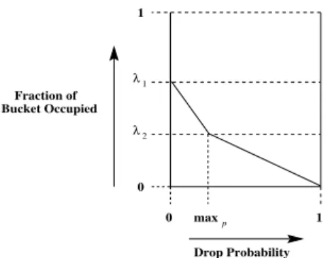
Selective Fair Early Detection (SFED) is an easy to implement rate control based active queue manage-ment discipline which can be coupled with any scheduling discipline. SFED operates by maintaining a token bucket for every flow (or aggregate of flows) as shown in Figure 2. The token filling rates are in proportion to the permitted bandwidths. Whenever a packet is enqueued, tokens are removed from the corresponding bucket. The decision to enqueue or drop a packet of any flow depends on the occupancy of its bucket at that time. The dependence of drop probability on the buffer occupancy is shown in Figure 3. The probability profile is explained in Section IV.
SFED ensures early detection and congestion notification to the adaptive source. A sending rate higher than the permitted bandwidth results in a low bucket occupancy and so a larger drop probability thus indi-cating the onset of congestion at the gateway. This enables the adaptive flow to attain a steady state and prevents it from getting penalized severely. However, non-adaptive flows will continue to send data at the same rate and thus suffer more losses.
Keeping token buckets for flows is different from maintaining an account of per-flow queue occupancy. The rate at which tokens are removed from the bucket of a flow is equal to the rate of incoming packets of that flow, but the rate of addition of tokens in a bucket depends on its permitted share of bandwidth and not on the rate at which packets of that particular flow are dequeued. In this way a token bucket serves as a control on the bandwidth consumed by a flow.
1 0 0 1 λ 1 2 λ Drop Probability maxp Bucket Occupied Fraction of
Fig. 3. Probability profile of dropping a packet for a token bucket
the recent past. This is because the token bucket occupancy increases if packets of a flow do not arrive for some time. Similarly, the bucket occupancy drops if packets of that flow are enqueued at a higher rate than the token addition rate. This is important for protocols such as TCP which leave the link idle and then send a burst in alternate periods. No packet of such a flow should be dropped if its arrival rate averaged over a certain time interval is less than the permitted rate. The height of the bucket thus represents how large a burst of a flow can be accommodated. As such, this scheme does not penalize bursty flows unnecessarily.
For the simplest case, all buckets have equal weights and each token represents a packet (see Figure 2),
the rate at which tokens are filled in a bucket is given by
! #"
tokens per second. where C is the outgoing link capacity in packets per second and"
is the number ofactiveflows. We say that a flow is active as long as its corresponding bucket is not full. Note that this notion of active flows is different from that in the literature [6], [2], [1], namely, a flow is considered active when the buffer in the bottleneck router has at least one packet from that flow. However, we will see later, that despite the apparent difference in the definitions of an active flow, the two notions are effectively similar. See remark in Section IV (A-5). The addition of tokens at the rate thus chosen, ensure that the bandwidth is shared equally amongst all the flows and no particular flow gets an undue advantage.
A flow is identified as inactive whenever while adding tokens to that bucket, it is found to be full. The corresponding bucket is then immediately removed from the system. Its token addition rate is compensated by increasing the token addition rate for all other buckets fairly. Similarly, the tokens of the deleted buckets are redistributed among other buckets.
The heights of all the buckets are equal and their sum is proportional to the buffer size at the gateway. Since the total height of all the buckets is conserved, during the addition of a bucket the height of each bucket decreases, and during the deletion of a bucket the height of each bucket increases. This is justified since if there are more flows a lesser burst of each flow should be allowed while if there are lesser number of flows a larger burst of each should be permitted.
During creation and deletion of buckets, the total number of tokens is conserved. This is essential since if excess tokens are created a greater number of packets will be permitted into the buffer resulting in a high queue occupancy while if tokens are removed from the system a lesser number of packets will be enqueued which may result in lesser bursts being accommodated and also lower link utilization in some cases.
IV. THEALGORITHM
With reference to the Figures 1, 2 and 3 we define the system constants and variables below.
Constants
B: Size of the buffer (in packets) at the gateway.
$
&% : This parameter determines the total number of tokens,
' , in the system. We take
% throughout the paper. ' %)(+* , %-,/.
Probability Profile 021 : It maps the bucket occupancy to the probability of dropping a packet when it
arrives.
The generality of the algorithm allows any probability profile to be incorporated. However, a probability profile is needed to detect congestion early and to notify the source by causing the packet to be dropped or marked (for ECN [8]). Figure 3 shows the probability profile used in our simulations. It is similar to the gentle variant of RED drop probability profile. We use the gentle variant of the RED probability profile as shown in Figure 3.
031 54 67 7 7 7 7 7 8 7 7 7 7 7 79 . : <;>=2? @BA ; CB1 3D $E =2?GF @ A D $E DH :5I ; =2? @ A ; : CB1KJ ML 1 33DH E =2?NF @OA DH . ;P=2? @OA ; :5I Global variables "
: Number of flows (equal to the number of buckets) in the system.
Q
: Maximum height of each bucket when there are"
active connections in the system,
Q
R
'
#"
S : Variable to keep account of the excess or deficit of tokens caused at deletion and creation of buckets.
During bucket addition and deletion, the total number of tokens in the system may temporarily deviate from its constant value' .
S is used to keep track of and compensate for these deviations.
Per-flow variables
BT : Occupancy of the bucket in tokens, .U
T U/Q
A. SFED Algorithm
The events that trigger actions at the gateway are: 1. Arrival of a packet at the gateway.
2. Departure of a packet from the gateway. 1. Arrival of a packet (flowid j)
If the bucketV does not exist
Create BucketV [Section IV-A-4]. Drop packet with probability
W 0 1 BT
If packet not dropped
T T LX
Enqueue packet in queue. 2. Departure of packet
The model shown in Figure 2 is valid only for fluid flows where the flow of tokens into the buckets is continuous. However, the real network being discrete due to the presence of packets, the model may be approximated by adding tokens into the system on every packet departure since the packet dequeue rate is also equal to C. When there are no packets in the system, i.e., every bucket is full, no tokens will be added into the system as required. We explain the steps taken on every packet departure.
S S J if SY,/. Z \[2^]_\`ba5c S [Section IV-A-3].
3. Token distribution
Tokens may be distributed in any manner to ensure fairness. One straightforward way is to distribute them in a round robin fashion as shown below.
while SYd
find next bucketV T T J S S L/ if bucketV is full
delete bucketV [Section IV-A-5].
4. Creation of bucketV
A bucket is created when the first packet of a previously inactive flow is enqueued thus increasing the flows to"
J
. The rate of filling tokens into each bucket isegf
! " J
. A full bucket is allocated to every new flow. It is ensured that the total number of tokens in the system remain constant. The tokens required by the new bucket are compensated for by the excess tokens generated, if any, from the buckets that were shortened. VariableS is maintained to compensate for the excess or deficit of tokens.
Increment active connections to "
J
.
Update height of each bucket toQ gf ' " J . T ' " J . S S L Q gf
For every bucket ih V if 54 ,/Q jf S S J 4 L Q jf k4 Q gf 5. Deletion of bucketV
A bucket is deleted when a flow is identified to be inactive thus reducing the number of flows to " Ll
. The rate of filling tokens into each bucket is increased tom
E ! " Ln
. It is obvious that the deleted bucket is full at the time of deletion. Variable S is maintained to compensate for the excess tokens created
so that the total tokens remain constant.
Decrement active connections to
"
LX
.
Update height of each bucket toQ
E ' " L/ . S S J Q
Remark: Note that by the nature of token distribution, if a packet is in position from the front of the
queue, the average number of tokens added to its bucket when the packet is dequeued is
=
. Therefore, when the bucket is full (and deleted), there is no packet in the buffer belonging to that flow. This is consistent with the existing definition of active flows.
We see that token distribution and bucket creation are"
steps. Hence, in the worst case, both enqueue and dequeue are"
operations. We now present the Randomized SFED Algorithm which is O(1) for both enqueue and dequeue operations. This extension makes the SFED algorithm scalable, and hence, practical to implement.
B. The Randomized SFED Algorithm (R-SFED)
We now propose the Randomized SFED algorithm that has O(1) average time complexity for both enqueue and dequeue operations.
1. Arrival of a packet (flowid j)
If the bucket
V does not exist
If T
,XQ
(to gather excess tokens)
S J T L Q T Q
Drop packet with probability
W 0 1 BT
If packet not dropped
T
T LX
Enqueue packet in queue. 2. Departure of packet
We explain the steps taken on every packet departure.
S S J Z ^[2^]_\`ba5c /o p f
where Q is the queue size. [Section IV-B-3]. 3. Token distribution
q o
p
f
buckets are accessed randomly. This means if we are short of tokens, i.e S
;
.
, then we grab tokens, else we add tokens. Any bucket which has more thanQ
tokens is deleted.
for i=1 to
q
do
Choose a random bucket j ifSr,/. T T J S S L/ else T T Ls S S J ifBT ,/Q
delete bucket j [Section IV-B-5]
Note thatS may be negative but it is balanced from both sides, i.e., when it is negative we try to increase it
by grabbing tokens from the buckets and when it is positive we add tokens to the buckets. The quantity q
is the upper bound on the work done in the token distribution phase. But generally, and as also observed in our experiments,q
is always close to 1. 4. Creation of bucketV
Increment active connections to
" J . UpdateQ gf ' " J . T ' " J . S S L Q gf
In Randomized SFED, we do not gather the excess tokens that might result in the buckets when we decrease the height. Hence, this procedure becomes O(1). Instead these excess tokens are removed whenever the bucket is accessed next.
5. Deletion of bucketV
Decrement active connections to
"
LX
.
Update height of each bucket toQ
E ' " L/ . S S Jt T
Every operation in the Randomized SFED Algorithm is O(1) in the amortized sense. This can be seen from the following observation. If u packets have been enqueued till now, then, the maximum number of
tokens added to the buckets over successive dequeues is also u , implying &
amortized cost for token distribution. All other operations such as bucket creation, deletion etc., are constant time operations.
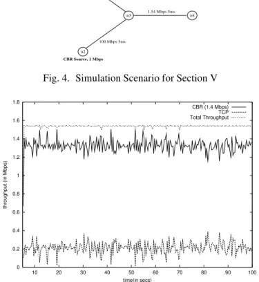
n4 1.54 Mbps 5ms n3 100 Mbps 15ms 100 Mbps 5ms CBR Source, 1 Mbps TCP Source n1 n2
Fig. 4. Simulation Scenario for Section V
0 0.2 0.4 0.6 0.8 1 1.2 1.4 1.6 1.8 10 20 30 40 50 60 70 80 90 100 throughput (in Mbps) time(in secs) CBR (1.4 Mbps) TCP Total Throughput
Fig. 5. Throughput vs time for RED algorithm Operating in byte mode
SFED can be easily implemented in the byte mode where each token represents a byte. Whenever a packet is enqueued tokens equal to the size of the packet are subtracted from the corresponding bucket and whenever a packet is dequeued corresponding number of tokens are added toS .
V. SIMULATIONRESULTS
We compare the performance of SFED with other active queue management algorithms in different net-work scenarios. RED and CHOKe are O(1) space algorithms and make use of the current status of the queue only to decide the acceptance of an arriving packet, whereas FRED keeps information corresponding to each flow. This makes FRED essentially O(N) space. SFED also keeps one variable per flow. This extra infor-mation per flow is made use of to provide better fairness. All simulations are done using Network Simulator (ns) [9]. We use FTP over TCP NewReno to model adaptive traffic and a Constant Bit Rate (CBR) source to model non-adaptive traffic. The packet size throughout the simulations is taken to be v
2w
Bytes. For RED and FRED, andC are taken to be
yx
and w
of the buffer size, respectively. The value of
1 is .O(+.
w
for RED, FRED and SFED. The values of :
and : I are w
and yx
for SFED. All values chosen for the algorithms correspond to those recommended by the respective authors.
Fair bandwidth allocation
The Internet traffic can broadly be classified into adaptive and non-adaptive traffic. We show the amount of fairness achieved by different queue management disciplines when adaptive traffic competes with non-adaptive traffic. Our simulation scenario is shown in Figure 4. The bottleneck link capacity is 1.54 Mbps (a T-1 link). The incoming flows consist of a CBR source sending data at the rate of 1.4 Mbps and a TCP source with no receiver window constraints. We chose the buffer size to be 24 packets. The graphs depicted in Figures 5, 6, 7 and 8 are for a time range of 5 to 100s. Figures 5, 6, 7 and 8 show the variation of throughput of TCP and CBR flows with time for the scenario shown in Figure 4. Since the bottleneck link
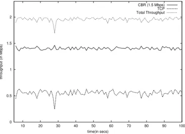
0 0.5 1 1.5 2 10 20 30 40 50 60 70 80 90 100 throughput (in Mbps) time(in secs) CBR (1.5 Mbps) TCP Total Throughput
Fig. 6. Throughput vs time for CHOKe algorithm
0 0.2 0.4 0.6 0.8 1 1.2 1.4 1.6 1.8 10 20 30 40 50 60 70 80 90 100 throughput (in Mbps) time(in secs) CBR (1.4 Mbps) TCP Total Throughput
Fig. 7. Throughput vs time for FRED algorithm
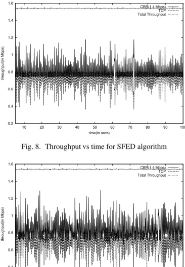
capacity is 1.54 Mbps, ideally both the flows should get equal share of bandwidth i.e., 0.752 Mbps. We observe that SFED performs better in terms of fairness since the throughput of both the flows are closest to the ideal.
It can be seen from Figure 7 that FRED consistently penalizes the TCP flow during a certain interval of simulation. This is evident from the separate bands of throughput of CBR and TCP in Figure 7. This is because the[^]z^{|c variable for the TCP flow is set but that of the CBR flow is not which is just the opposite
of what should happen.
}~
is the bandwidth delay product, which is 16 packets for this scenario. Now we vary the buffer size from
I
}~
to }~
and observe the performances of all four schemes. To compare performance of various algorithms, we have chosen a fairness coefficient (] ) [14], which is defined as
] 4N `b4 I " 4N ` I 4
where`b4 is the bandwidth obtained by the flow and
"
is the number of flows. It gives a measure of the amount of fairness achieved. Table I shows the percentage of throughput obtained by the TCP flow for all the schemes while Table II shows the fairness coefficients. From table I, it is clear that SFED consistently performs better than RED, CHOKe and FRED across a wide range of buffer sizes. It protects the adaptive TCP flow better than RED, CHOKe or FRED while still maintaining a high link utilization. SFED consis-tently outperforms RED and CHOKe at all buffer sizes. It also performs as well as FRED at high buffer sizes while it at low buffer sizes it is much better than FRED. FRED shows poor fairness characteristics at
0.2 0.4 0.6 0.8 1 1.2 1.4 1.6 10 20 30 40 50 60 70 80 90 100 throughput(in Mbps) time(in secs) CBR(1.4 Mbps) TCP Total Throughput
Fig. 8. Throughput vs time for SFED algorithm
0.2 0.4 0.6 0.8 1 1.2 1.4 1.6 10 20 30 40 50 60 70 80 90 100 throughput(in Mbps) time(in secs) CBR(1.4 Mbps) TCP Total Throughput
Fig. 9. Throughput vs time for Randomized SFED algorithm
low buffer sizes. This is because the FRED per flow[\]_\{|c variable is set at each TCP burst due to the small
buffer size. This causes TCP to be penalized heavily.
From tables [I,II], we observe that Randomized SFED performs almost as good as SFED. Since Random-ized SFED has lower time complexity than SFED, it is only appropriate to use RandomRandom-ized SFED rather than SFED. From now on, any reference to SFED implies Randomized SFED.
Adaptation to a dynamically changing scenario
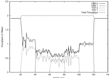
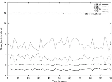
In Figure 10 we show how SFED adapts in a situation where the number of flows keep on changing. There are 2 CBR sources namely
* and *
of rates 1.9 Mbps each and 2 TCP sources namely' }) and' } . * and *
start at times 0 and 40 seconds, respectively, while' }
and' }
start at times 20 and 60 seconds, respectively.
* and *
finish at times 140 and 120 seconds while' }
and' }
finish at times 80 and 100 seconds, respectively. We observe from Figure ( 10) that as the number of active flows increase, the share of each flow decreases dynamically and vice versa.
Protection for fragile flows
Flows which are congestion aware, but are either sensitive to packet losses or slower to adapt to more available bandwidth are termed fragile flows [2]. A TCP connection with a large round trip time (RTT) and having a limit on its maximum window fits into this description.
TABLE I
BANDWIDTH PERCENTAGE OBTAINED BYTCPAT VARIOUS BUFFER SIZES I }~ }~ I }~ w }~ }~ RED 12.9% 14.8% 13.9% 14.1% 12.4% CHOKe 32.0% 34.4% 37.0% 36.2% 36.0% FRED 22.2% 32.1% 39.7% 45.9% 47.1% SFED 37.3% 40.1% 44.1% 45.8% 47.1% R-SFED 35.7% 39.2% 43.8% 45.5% 46.8% TABLE II
FAIRNESS COEFFICIENTS OBTAINED AT VARIOUS BUFFER SIZES I }~ }~ I }~ w }~ }~ RED 0.642 0.668 0.655 0.660 0.639 CHOKe 0.777 0.793 0.842 0.851 0.838 FRED 0.764 0.887 0.959 0.993 0.996 SFED 0.939 0.961 0.986 0.993 0.996 R-SFED 0.925 0.956 0.985 0.992 0.996
and non-fragile sources. The simulation scenario is shown in Figure 11. The TCP source originating at node
x
is considered a fragile flow due to its large RTT of 40ms, while the
'M' s for the other three flows is
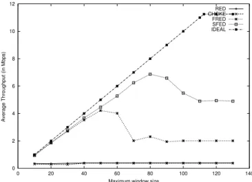
6ms. The CBR flow sends data at a rate of 40 Mbps. Since there are 4 flows in the system and the bandwidth of the bottleneck link is 45 Mbps, ideally each flow should receive its fair share of 11.25 Mbps. We vary the maximum allowed window size, , for the fragile flow and observe the throughput obtained by this flow.
The maximum achievable throughput is then given by5g
= ( z 'M' where
is the packet size and
'M' is the round trip time. The maximum throughput is thus a linear function of the maximum window
size. The RTT for the fragile flow is taken to be since we can safely ignore the queueing delays due to the large bandwidth (45 Mbps) of the outgoing link. Ideally, the maximum throughput should never exceed 11.25 Mbps, i.e., it should increase linearly until 11.25 Mbps, and should then stabilize at 11.25 Mbps. This ideal bandwidth share is shown in Figure 12.
As can be observed from Figure 12, SFED provides bandwidth allocation for the fragile flow almost as good as in the ideal case. For a small maximum window size, every algorithm is able to accommodate the bursts of the fragile flow without any drops, but with increasing maximum window size, packet drops result in drastic reduction of the fragile flow throughput. A packet drop is fatal for a fragile source as it is slow in adapting to the state of the network. We see that the throughput becomes constant after a while since the window size of the fragile source is not able to increase beyond a threshold. Therefore, no matter how large the maximum window size is increased beyond this threshold the throughput does not increase and thus approaches a constant value. This constant value is much less than its fair share 11.25 Mbps due to the less adaptive nature of fragile flows.
In the Appendix, we analyse SFED using a simplified stochastic model. We show that SFED facilitates fair bandwidth sharing at a gateway in the presence of a mix of adaptive and non-adaptive traffic when adequate buffering is provided.
VI. GENERALIZATIONS OFSFED
The SFED algorithm can be easily modified for scenarios such as weighted flows, differentiated services of aggregate flows and hierarchy of flows.
0 0.5 1 1.5 2 2.5 20 40 60 80 100 120 140 throughput (in Mbps) time(in sec) CBR 0 CBR 1 TCP 0 TCP 1 Total Throughput
Fig. 10. Performance of SFED in a dynamically changing scenario with bottleneck link capacity 2 Mbps
n5 45 Mbps 2ms n6 n2 n4 100 Mbps 18ms CBR Source, 40Mbps TCP Source n1 n3 TCP Source 100 Mbps 1ms 100 Mbps 1ms Fragile TCP Source 100 Mbps 1ms
Fig. 11. Simulation scenario with a fragile flow SFED with Weighted Flows
SFED can be easily adapted for bandwidth sharing among flows with different weights. Assuring fairness now means allocating bandwidth to each flow in proportion to its weight. By setting the bucket height and the share of token addition rate for each flow in proportion to its weight, the desired bandwidth allocation can be obtained.
We redefine the parameters for the weighted version of SFED as:
4: Weight of the flow.
4: Normalized weight of flow 4 B4 4, j active connection HeightQ 4 of bucket =M4 %)(+*
Token filling rate
4 for bucket =M4
SFED with Aggregate Flows
In the recent past, much work has gone into providing differentiated services [17] to flows or flow aggre-gates. Connections with similar properties and requirements can be aggregated and considered as a single flow.
Aggregation can be done in many ways depending on the requirements. One way to aggregate flows is by the nature of traffic they carry, i.e., all streaming audio and UDP traffic into one flow, all FTP, HTTP and web traffic in another while all telnet, rlogin and similar interactive traffic in a separate flow.
SFED can be used effectively for bandwidth allocation among aggregate of flows. Multiple connections can be aggregated as a single flow in SFED and weighted according to their requirements. A set of con-nections, aggregated as a single flow has a single token bucket. Among flows within an aggregate, SFED behaves much like RED.
0 2 4 6 8 10 12 0 20 40 60 80 100 120 140
Average Throughput (in Mbps)
Maximum window size
RED CHOKE FRED SFED IDEAL
Fig. 12. Performance of the fragile flow with increasing receiver window constraint (gateway buffer size = 96 packets)
0.15 0.2 0.25 0.3 0.35 0.4 0.45 0.5 0.55 0.6 0 10 20 30 40 50 60 70 80 90 100 Throughput (in Mbps)
Time (in secs)
CBR 0 CBR 1 TCP 0 TCP 1 TCP 2
Fig. 13. Performance of SFED with flow Aggregation
Mbps. Two CBR flows of sending rates 1 Mbps each are clubbed into one aggregate while 3 TCPs into another. The combined throughput for all TCP flows or all CBR flows should be 1 Mbps which is nearly so. The observed performance of individual connections within an aggregate is because SFED behaves much like RED for flows constituting a flow aggregate. This behaviour can be easily remedied by hierarchical flow aggregation which we discuss in the next section.
SFED with Hierarchical Flows
Besides simple aggregation of flows, it is also desired to have fair bandwidth sharing amongs hierarchical flows i.e., multiple levels of flow distinction. For example, we would like to distinguish flows first on the basis of the traffic content and then amongst each kind of traffic, on the basis of different source and destination IP addresses. This provides a two level of hierarchy of distinguishing flows.
A hierarchical classification of flows can be represented by a tree structure where a leaf node represents an actual flow, while an interior node represents a class of flows or other classes. Each node has a weight attached to it such that the weight of each interior node is the sum of the weights of its children. If one of the flows is not using its full share of bandwidth, then the “excess” bandwidth should be allocated to its sibling flows, if possible. Otherwise this “excess” is passed on to its parent class for redistribution among its siblings and so on.
This sort of scenario is easily implementable using SFED. In such a hierarchy tree of flow classification, we assign a bucket each for the different leaves of the tree. The key distinction here is that at a flow addition
TCP CBR 75% 25% 67% 33% 33% 67% CBR1 CBR0 TCP1 TCP0 12 Mbps
Fig. 14. The bandwidth sharing hierarchy tree for Section VI
0 2 4 6 8 10 12 14 0 10 20 30 40 50 60 70 80 90 100 Throughput (in Mbps)
Time (in secs)
CBR 0 CBR 1 TCP 0 TCP 1 Total Throughput
Fig. 15. Performance of SFED with Hierarchical Flows
or deletion the adjustment of tokens and heights would be done at a level closest to the that flow and this redistribution will move upwards from the leaves to the root. The first level of redistribution of tokens of a flow would be at the same level i.e., among its siblings. The overflow of tokens from this subtree will then be passed over to its sibling subtrees in the hierarchy and so on.
Figure 15 shows the performance of SFED for a scenario whose hierarchy tree for bandwidth sharing is shown in Figure 14. The bottleneck link bandwidth is 12 Mbps, so ideally CBR and TCP classess should obtain bandwidths of 3 Mbps and 9 Mbps respectively. Among the individual flows,
* and *
have shares of 2 Mbps and 1 Mbps respectively, while TCP0 and TCP1 should get bandwidths of 6 Mbps and 3 Mbps, respectively. From Figure 15, it is clear that SFED distributes bandwidth fairly among both classes. We also note that whenever the throughput of one of the TCP flows dips, the excess bandwidth is utilized by the other TCP connection, which should be the case. Excess bandwidth can be utilized by the CBR aggregate only when the throughputs of both the TCP flows are low.
VII. CONCLUSIONS ANDFUTUREWORK
We have proposed SFED: a rate control based queue management discipline at the Internet Gateways. Through simulations, we have compared SFED with other well known congestion avoidance algorithms such as RED, CHOKe, FRED, and, have shown that SFED achieves a fair bandwidth allocation amongst competing (adaptive and non-adaptive) flows across a much wider range of buffer sizes at a bottleneck router. We then proposed a scalable version of SFED using randomization that has an O(1) time complexity. One area of future work is to compare SFED with some other recently proposed active queue management algorithms in the literature, such as Balanced RED (BRED) [4] and Stochastic Fair Blue (SFB) [5]. Finally, from a complexity perspective, it will be interesting to explore reduction of space to
"
, say&b "
, and still achieve performance comparable to
"
REFERENCES
[1] S. Floyd, V. Jacobson, “Random Early Detection Gateways for Congestion Avoidance”, IEEE/ACM Transactions on Net-working, Vol. 1, No. 4, August 1993.
[2] D. Lin, R. Morris, “Dynamics of Random Early Detection”, In Proceedings of ACM SIGCOMM, 1997.
[3] R. Pan, B. Prabhakar, K. Psounis, “A Stateless Active Queue Management Scheme for Approximating Fair Bandwidth Allo-cation”, In Proceedings of IEEE INFOCOM’2000, Tel-Aviv, Israel, March 26-30, 2000.
[4] F.M. Anjum, L. Tassiulas, “Balanced-RED: An Algorithm to achieve Fairness in the Internet”, In Proceedings of IEEE IN-FOCOM’1999.
[5] W. C. Feng, D. Kandlur, D. Saha and K. Shin, “Blue: A New Class of Active Queue Management Algorithms”, Technical Report CSE-TR-387-99, University of Michigan, April 1999.
[6] B. Suter, T.V. Lakshman, D. Stiliadis, A. Choudhury, “Efficient Active Queue Management for Internet Routers”, Proc . INTEROP, 1998 Engineering Conference.
[7] S.M. Ross, “Introduction to Probability Models”, Academic Press, 1997.
[8] S. Floyd, “TCP and Explicit Congestion Notification”, Computer Communications Review, 24(5), Oct 1994. [9] S. McCanne, S. Floyd, “ns-Network Simulator”, http://www-nrg.ee.lbl.gov/ns/
[10] V. Jacobson and M.J. Karels, “Congestion Avoidance and Control”, In Proceedings of ACM SIGCOMM, 1988. [11] S. Floyd and V. Jacobson, “On Traffic Phase Effects in Packet Switched Gateways”, Comp. Comm. Review, April 1991. [12] H. Zhang, S. Shenker and I. Stoica, “Core-Stateless Fair Queueing: Achieving Approximately Fair Bandwidth Allocations in
High Speed Networks”, In Proceedings of ACM SIGCOMM, September, 1998, Vancouver, BC, Canada.
[13] F. Kelly, “Charging and rate control for elastic traffic”, European Transactions on Telecommunications, Vol 8, 1997. [14] L. L. Peterson and B. S. Davie,Computer Networks: A Systems Approach, Morgan Kaufmann Publishers, Inc., 1996. [15] S. Floyd, V. Jacobson, “Link Sharing and Resource Management Models for Packet Networks”, IEEE/ACM Transactions on
Networking, Vol. 3 No.4, August 1995.
[16] D.D. Clark, “Explicit Allocation of Best-Effort Packet Delivery Service”, IEEE/ACM Transactions on Networking, Vol.6, August 1998.
[17] K. Nichols, “Definition of Differentiated Services Behavior Aggregates and Rules for their Specification”, Internet Draft, Differentiated Services Working Group, IETF.
APPENDIX
Analysis of SFED
In this section, we show that SFED facilitates fair bandwidth sharing at a gateway in the presence of a mix of adaptive and non-adaptive traffic. We assume that if a token bucket for a flow becomes full, it is marked inactive, but is not deleted. Its token addition rate is distributed among other active flows. On arrival of a packet of that flow, the bucket is again marked active. A token arriving at a bucket is either added to the bucket, if the bucket is not full, else it overflows and is added to some other non-full bucket. The key insight we exploit is that over large periods of time the throughput obtained by a flow is equal to the number of tokens added to its token bucket. Let
denote the rate in tokens/s at which tokens arrive at all the token buckets. We consider the equivalent of fluid flow token distribution where
tokens per second arrive at the buckets continuously and! #"
tokens fall into each bucket per second. The inter arrival time of tokens into a bucket is then"& K
. If all the buckets are full, then the arriving tokens are simply thrown away. Now if"
denotes the number of active connections andW
4 denotes the fraction of tokens that overflow from the
token bucket, then the throughput,4 of flow is given by 34 ! #" 3iL W 4 (1) Our analysis focuses on showing thatW
4 is small for both adaptive and non-adaptive flows.
We first consider the case of non-adaptive CBR traffic. If the rate of arrival of packets of the flow is higher than the token addition rate, then eventually the bucket occupancy decreases and enters the region where the loss probability is positive. The bucket occupancy oscillates about a certain height D (
.U D U : Q ). In this case, the bucket is never full and W
4
.
, which implies that the flow obtains its fair share of bandwidth. On an average, for a CBR flow with arrival rate: , the fraction of packets dropped are given by
1 - ! #"
:
If the rate of arrival of CBR packets is less than the rate of addition of tokens, then the bucket will almost always remain full. Every arriving packet of the CBR flow will find a token available, and so this flow will get the whole of the bandwidth it needs.
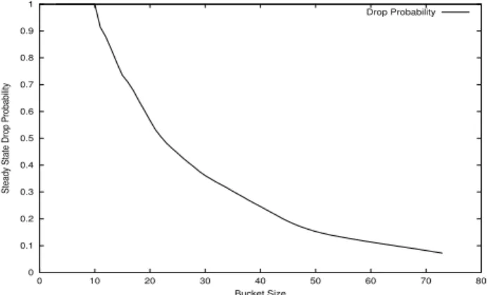
0 0.1 0.2 0.3 0.4 0.5 0.6 0.7 0.8 0.9 1 0 10 20 30 40 50 60 70 80
Steady State Drop Probability
Bucket Size
Drop Probability
Fig. 16. Drop Probability vs bucket size for a TCP flow with RC/N=10,y
1. Total number of flows remain the same during the period of analysis.
2. The TCP connections are in a congestion avoidance phase in which the window increases by a one every RTT on successful transmission of the entire window.
3. The TCP version is New Reno in which the window drops by half for one or more drops in a window. 4. The round trip time (RTT) of TCP connections is constant and denoted by
. For simplicity we assume that
is a multiple of token inter-arrival time"& K
.
5. The TCP data arrives in bursts of size of a window and is processed immediately.
These assumptions can be relaxed, however at the expense of greater technicality in analysis. We discuss some of these extensions later.
These assumptions allow us analyze each bucket independently. The height of the bucket of each flow is
Q
. Let¡ denote the minimum buffer occupancy above which no drop is possible i.e.,¡
£¢¥¤ 0 1 £¢¦ .
. For the probability profile in Figure 3,¡
:
)
Q
. Consider one bucket associated with a TCP flow. Let§¨ denote its buffer occupancy level just before the arrival of© burst and let ªt¨ denote the window
size at this instant. Then the collection of random variables(rv)
§¨¬«bª¨ !®
d¯.
is a finite state space Markov chain. The rv§&¨ takes integer values from
. toQ
whileª°¨ takes integer values from . toQ
J
(initially, the window size may be greater than Q
J
, but once it decreases below this level it can never thereafter exceed it). Let
denote the state space of §±¨k«bª¨
. To describe the transition matrix for this Markov chain, we first need to evaluate the probability of droppingZ
packets on arrival of a burst of size ,
when the bucket occupancy is . Call this
W ²«« Z . Note thatW ²«« . whenever L d ¡ and ,
¡ . For other values, this probability may be evaluated using the recurrence relation
W «« Z 031 ( W ²« Ls « Z L/ J <L 031 ( W L/ « L/ « Z (2) where 031
is the dropping probability of a packet when the bucket occupancy is . Now the transition
probability matrix may be determined by noting that
§¨ f «bª°¨ f ´³2C²³2§¨ L ª¨!J Z « .Bµ J ¶ #" « Q µ «bª¯·· (3) with probabilityW §¨¬«bª¨k« Z , where.U Z U ª¨ andª ·· is ª°¨!J forZ . and ª°¨ w otherwise. If ¹¸ « ®g «
denotes the matrix of steady state probabilities of the Markov chain then let
4 º» ¸ Q «
. We now show that 4 is an upper bound on
W
4.
Consider M consecutive window burst arrivals. Let ¼/½ denote the number of bursts that see the bucket
full on arrival. Clearly, ¾N¿NÀ&ÁÂÃs¼n½ ¼
4. Similarly, let '
denote the number of token arrivals to
the bucket during the ¼ window burst arrivals and let ' ½ denote the number of these arrivals that find
the bucket full i.e., they overflow. Then ¾N¿NÀÄÁÂÃY' ½ '
W 4. Now ' ¼ ! #" . Note that whenever a token sees the bucket full, the next window arrival must also find the bucket full. This implies that' ½ U ¼Y½ ! #" . The relation4 d W
4 then follows. So finally, we get
W 4 U º» ¸ Q « .
Figure 16 shows this probability obtained by numerically solving the Markov chain for different values of bucket size Q
(see, for example [7], for a discussion on Markov chains and on computation methods for stationary probabilities). It can be seen that°4 is approximately an exponentially decreasing function of the
buffer sizeQ
. In fact we now argue that for large enoughQ
,4 and hence
W
4 equals
. , i.e., there exists
an upper threshold for the bucket occupancy. Suppose that § E m; ¡ U § and ª
. From this instant till bucket occupancy becomes less
than¡ , the evolution of the Markov chain is deterministic since there cannot be any packet drops. Note that §
U
¡J
! #"
since at most RC/N tokens can be added in an RTT interval. Now the bucket length goes up at instant /J ifª ; ¶ #"
and continues to increases as long as the window size is less than the token arrivals during an RTT, i.e.,! #"
. Since the window increases by 1 after every RTT, eventually the bucket occupancy begins to decrease. The maximum level reached is clearly a decreasing function of .
Hence the maximum bucket occupancy is achieved for
.
. Thus the maximum bucket occupancy occurs after ÆÅ£! #" J 3Ç 'M' s and when§ ¡´J ! #" . For no overflow,Q d § f ¨ . Thus for4 and henceW
4 to be zero, the following inequality should hold
Q d w ! #" I J w ¶ #" Jn¡ (4)
This means that given a sufficiently large bucket Q
, a TCP flow is always able to use its fair share of bandwidth.
Another noteworthy point is that since bucket size is proportional to the buffer size * at the gateway,
then increasing the bucket size and hence increasing *
, may lead to increase in queuing delays so that the assumption that RTT is a constant may no longer be realistic. As a first order approximation we model
as a linear function of* , i.e.,
¯ JnÈ
* , where !
is the propagation delay (assumed to be constant) and
È
*
denotes the queueing delay. Q
and¡ are proportional to
*
and so the Inequality 4 becomes quadratic in* as follows: w J-È * ¶ #" I J w J-È * ! #" UXɦ*Ä( (5) whereÉ is an appropriate constant. Clearly ( 5) does not hold for large* indicating that for* large enough
and hence the RTT large enough, the buffer will overflow. inequality ( 5) can be solved to obtain the range of *
for which the TCP flow is always able to obtain its fair share of bandwidth. The parameter È is a
representative of the queuing delays. Calculating the appropriate value for È is a problem which needs
further research.
Connections having large
'M' have large overflow probabilities as indicated by 5. Hence, TCP flows
with large
'M' s, are unable to obtain their fair share of bandwidth. The notion of “proportional fairness”
amongst TCP flows with different
'M' s has been discussed in [13] where they justify the low bandwidth
allocation to connections with large '<' s.