The Conditional CAPM, Cross-Section Returns and Stochastic Volatility

(1)

MPRA

Munich Personal RePEc Archive

The Conditional CAPM, Cross-Section

Returns and Stochastic Volatility

Ka Wai Terence Fung and Chi Keung Marco Lau and Kwok

Ho Chan

United international College - Beijing Normal University and Hong

Kong Baptish University, Northumbria Unversity, United

international College - Beijing Normal University and Hong Kong

Baptish University

2013

Online at

http://mpra.ub.uni-muenchen.de/52469/

(2)

The Conditional Equity Premium, Cross-Sectional Returns and Stochastic

Volatility

Ka Wai Terence Fung Chi Keung Marco Lau

&

Kwok Ho Chan

Abstract

Bansal and Yaron (2004) demonstrate, by calibration, that the Consumption-Based Capital Asset Pricing Model (CCAPM) can be rescued by assuming that consumption growth rate follows a stochastic volatility model. They show that the conditional equity premium is a linear function of conditional consumption and market return volatilities, which can be estimated handily by various Generalized Autoregressive Conditonal Heterskedasticity (GARCH) and Stochastic Volatility (SV) models.We find that conditional consumption and market volatilities are capable of explaining cross-sectional return differences. The Exponential GARCH (EGARCH) volatility can explain up to 55% variation of return and the EGARCH model augmented with -a cointegrating factor of consumption, labor income and asset wealth growth- greatly enhance model performance. We proceed to test another hypothesis: if Bansal and Yaron estimator is an unbiased estimator of true conditional equity premium, then the instrumental variables for estimating conditional equity premium should no longer be significant.We demonstrate that once the theoretical conditional risk premium is added to the model, it renders all instrumental variables redundant. Also, the model prediction is consistent with observed declining equity premium.

JEL Codes: E21; G1; G12

Keywords: Financial Economics, Macroeconomics and Monetary Economics, Equity Premium Puzzle, Fama-French Model



Division of Business and Management, United International College, Zhuhai, China [email protected]

_{Newcastle Business School, Northumbria University, Newcastle upon Tyne, UK.}

[email protected]

_{Division of Business and Management, United International College, Zhuhai, China}

(3)

1. Introduction

Financial derviatives can be priced in two methods - relative pricing and absolute pricing. Financial engineers, on the one hand, price a financial instrument by forming a replicating portfolio. The cash flow of a call option, for instance, can be replicated by holding stock shares and shorting bonds. The option is priced relative to the market prices of those two assets. Financial economists, on the other hand, explore the links between asset returns and macroeconomic variables which are the sources of systematic risk. One of the early attempts is the Sharpe-Lintner-Black Capital Asset Pricing Model (CAPM), in which excess return of market portfolio is the common factor that explains cross-sectional return differences. In a two period model with exogenous labor income, the equity premium is proportional to the aggregate consumption growth, in which the multiplicative factor is elasticity of intertemporal substitution of consumption. This is the famous Consumption Based Capital Asset Pricing Model (CCAPM).

In spite of the theoretical simplicity and elegance of CAPM; when faced with empirical testing, it fails miserably. For instance, Banz (1981) identifies the small firm effect - small cap stocks and value stocks have unusually high average returns, while the return of large and growth stocks are lower than what CAPM predicts. Fama and French (1993) demonstrate that CAPM virtually has no power in explaining cross-sectional return when sorted by size and book-to-market ratios. Fama and French (1993) advocate a three factor model - market return, the return of small less big stocks (SMB), and the return on a portfolio of high book-market value stocks less low book-book-market value stocks (HML). The Fama and French (1993) model is a resounding success; however, it is still not clear how these factors relate to underlying macroeconomic risk. In fact, the independence and economic interpretation of SMB and HML remain as a source of controversy.

An alternative to the Fama and French (1993) model is the macroeconomic factor model, in which the factors are observed macroeconomic variables that are assumed to be uncorrelated to the asset specific error. The Chen et al. (1986) multi-factor model is one of those. They construct surprise variables by using the Vector Autoregressive Model (VAR). The VAR residuals of several macroeconomic variables, for example, Consumer Price Index (CPI), industrial production growth and oil price are used as uncorrelated macroeconomic variables. While the uncorrelatedness of those macroeconomic variables is less controversial, the explanatory power is unsatisfactory especially when compared to Fama and French (1993) model.

Jagannathan and Wang (1996) attribute the failure of CAPM to two reasons. First, CAPM holds in a conditional sense, not unconditionally. The stochastic discount factor is linear as stated in CAPM, but the coefficients are time varying. The static specification of market premium fails to take into account the effect of time-varying investment opportunities

(4)

in the calculation of asset risk. For instance, the betas of firms with relatively higher leverage rise during recession; firms with different types of assets will be affected by the business cycle in different way and to a different extent. Second, the return on value-weighted portfolio of all stocks is a bad proxy to wealth return. As a matter of fact, Roll (1977) argues that the market return cannot be adequately proxied by an index of common stocks. The problems are rectified by estimating a conditional version of CAPM and including human capital return, as an instrumental variable, in the model. They argue that with certain assumptions about the stochastic conditional expected excess return on zero-beta portfolio and conditional market risk premium, cross-section return can be written as a linear combination of factors with constant coefficients1. The Jagannathan and Wang (1996) model significantly improves predictive power of CAPM.

Lettau and Ludvigson (2002) resurrect the CCPAM. Along the line of Jagannathan and Wang (1996), they examine a conditional version of CCAPM, in which the stochastic discount factor is expressed as a conditional or scaled factor model. They model time-variation in the coefficients by interacting consumption growth with an instrument, in particular, a cointegrating factor - a cointegrating residual between consumption, asset(nonhuman) wealth, and labor income (all in log). A growing literature find that expected excess returns on aggregate stock market indice are predictable, suggesting that risk premium varies over time2. The parameters in the stochastic discount factor will then depend on investor’s expectations of future excess return. Lettau and Ludvigson (2001) demonstrate that drives time-variation in conditional expected return. While the consumption cointegrating factor alone fails to capture variation of average returns, they show that the interaction between and labor income growth or consumption growth can explain 70% variation of average return, it remains a difficult task to reconcile how this interaction term can make such a difference.

In this paper, we undertake the investigation of the CAPM by using a conditional market premium derived from an optimization-based model. Declining consumption volatility has been a plausible explanation for the declining equity premium. Bansal and Yaron (2004, hereafter referred to as the BY model) justify the equity premium by assuming that consumption growth rate follows a stochastic volatility model. They show that the conditional equity premium is a linear function of conditional consumption and market return volatilities. Thereafore, we proceed to estimate two stochastic volatility models to test the validity of BY model. Meanwhile, estimation methods of conditional volatility abound in the econometrics literature; for instance, the large class of Generalized Autoregressive Conditional Heteroskedasticity (GARCH) models. We will apply the Fama-MacBeth

1_{The proof can be found at the appendix of Jagannathan and Wang (1996).} 2_{see Campbell (1991) and Lamont (1998)}

(5)

approach to test the validity of the BY model using 25 Fama-French portfolios (U.S.A) sorted by size and book-to-market value. A couple questions will be addressed in the following sections. Once the ex-post market risk premium is replaced by conditional consumption and market return volatilities, does it improve the predictive power of CAPM? Is this study robust that different GARCH models give similar results? Furthermore, the following null hypothesis will be tested: if the theoretical BY equity premium is adequate, it would render the instrumental variables redundant.

The first procedure is the estimatin of conditional consumption and market volatilities by GARCH, Exponential GARCH (EGARCH), Threshold GARCH (TGARCH) and two stochastic volatility models. The predicted volatilities will then be used as factors for the second-step Fama-MacBeth procedure. Since we will compare the model performance to the conventional CAPM, Fama-French (1993) and Lettau and Ludvigson (2001) models, the U.S 25 Fama-French portfolio returns sorted by size and book-to-equity value will be used.

We find that the Bansal and Yaron theoretical premium significantly outperforms traditional CAPM using observed market premium. Using GARCH consumption and market volatility alone can explain 55% variation of cross-section return difference. Not only does it improve the Fama and French model, by replacing the ex-post market risk premium with the Bansal and Yaron (2004) premium, the Lettau and Ludvigson (2001) model also outperforms the former. Moreover, various _2_{tests reject the joint significance of Lettau and Ludvigson}

instrumental variables.

There are two contributions of this research. 1. We found supportive evidence to a general equilibrium model with the potential to resolve the equity premium puzzke. 2. Our statistical method is more straight forward than the existing literature – which are mostly calibration instead of statistical estimation- on the Bansal and Yaron (2004) model.

This paper is structured as follows. Section 2 outlines the Bansal and Yaron model. We briefly describe the derivation of the theoretical market premium. Section 3 is devoted to modelling conditional volatilities. Two Stochastic Volatilities and three typical GARCH type volatilities are estimated: Generalized Autoregressive Conditional Heteroskedasticity (GARCH), Exponential GARCH and Threshold GARCH. The idea is that if the Bansal and Yaron premium can truly explain cross-sectional return differences, the result should be applied to various conditional volatility specifications. Section 4 delineates the estimation equations. Section 5 reports the results and section 6 concludes.

2. Outline of Bansal and Yaron (2004) Model

We now consider the Bansal and Yaron (2004) model. It shows that, if consumption and dividend growth rate contain a small long-run predictable component, consumption volatility

(6)

is stochastic, and, if the representative household has Epstein and Zin preference, the asset and return premium will be a linear function of conditional consumption and market volatility. The Euler condition is given by

1 = ] [ ₁ _,(1_₁ ) _,_₁   at it t t G R R E      (1)

where  is the discount factor, Gt1 is gross return of consumption, Ra,t1 is the gross

return on an asset that delivers aggregate consumption as its dividends each period, and R_i_,_t_₁ is the individual asset return. As well-documented in the literature, this class of preference disentangles the relation between intertemporal elasticity of substitution (IES) and risk aversion. The parameter

   1 1 1 =  

, with 0 as the degree of risk aversion,  denotes IES.

Campbell and Shiller (1988) show that the log-linearized asset return (r_a_,_t_₁) can be expressed as 1 1 1 0 1 ,t =  t  t  t a z z g r   (2)

where ₀and ₁are constants; =log( )

t t t

C P

z is the log price-consumption ratio, and g_t_₁ is the log return of consumption. The log-linearized first order euler condition is

1 , 1 1= log  ( 1)    t   at t g r m      (3)

where mt1 is the stochastic discount factor. When =1, then  _

1

= , and the above equation is pinned down to the case of Constant Elasticity of Subsitution (CES) utility function. Moreover, if  =1 and  =1, we get the standard case of log utility. In the spirit of neo-classical Real Business Cycle model (RBC), an exogenous i.i.d shock perturbs consumption and output from their steady paths. The system of shocks is

1 1=   t  e t t t x e x    1 1 =    t  t t t x g   1 1 ,t = d  t  d t t d x u g     1 2 2 1 2 2 1= ( )    t   w t t      w 

(7)

(0,1) ,

, ₁ ₁ ₁

1 w u N

e_t_ _t_ _t_, _t_ ~

This system of equation suggests that consumption (g_t_₁) and dividend growth rates(g_d_,_t_₁

) are driven by an unobservable process x_t, and the volatility of the latter exhibits mean-reversion () but perturbed by an i.i.d shock (e_t_₁)3. Bansal and Yaron (2004) solve the log price-consumption ratio by method of undetermined coefficients, and find that

2 2 1 0 = _t _t t A Ax A z    (4) ) (1 ] ) ( ) 0.5[( = , 1 1 1 = 1 1 2 1 1 2 2 1 1 _ __               A _e A A

There are two noteworthy features of this model. First, if  and  are larger than 1, then

 is negative, and a rise in volatility lowers the price-consumption ratio, since the intertemporal effect dominates the substitution effect. Second, the risk premium is a positive function of the volatility persistence parameter ; meaning that the representative consumer dislikes a prolonged period of consumption shocks. After some algebra, the market premium in the presence of time-varying economic uncertainty takes the form:

) ( 0.5 = ) ( m_,t₁ f_,t m_,e m_,e t2 m_,w m_,w w2 t m_,t₁ t r r var r E       (5) where 2 t  and 2 w

 are the conditional consumption and wealth volatilities;  is the price of risk, and  is the quantity of risk. The risk premium of any asset, given by CAPM, can be expressed as t t m t t e m e m t f t i t r r var r E(   )=   0.5 ( ,1) 2 , , , 1 , (6)

The BY model calls for estimation of two equations. Equation (5) states that long-run market risk premium is determined by conditional consumption and market return volatility. In particular, the cointegrating vector is (_m_,_e_m_,_e,0.5). This paper focuses on equation (6),

3

(8)

which explains cross-sectional return differences by conditional volatilities.

The essence of the BY model is that persistent stochastic volatility can explain risk premium. Here we provide an empirical test, by regressing cross-sectional return against different variants of conditional stochastic volatility. Choosing the best stochastic volatility model is not the purpose of this paper. Rather, we want to show that if equation (6) can be explained by some common GARCH and SV models, it should provide indirect support for the BY model. More importantly, it provides an alternative for the Fama-French model. While the independence of Fama-French factors is controversial, aggregate consumption and market return volatilities should be uncorrected. Next section is devoted to the description of various conditional volatility models.

3. Volatility Modelling

This section outlines the three GARCH and two SV models considered in this study. Since the literature on conditional volatility is well-documented, the readers can refer to Bollerslev et al. (1992), Bollerslev et al. (1994) for a survey of the GARCH processes. We will also use the Exponential GARCH (EGARCH) and Threshold GARCH (TGARCH) to model asymmetry. Stochastic Volatility (SV) models which are reviewed in, for example, Taylor (1999), Ghysels et al. (1996) have been increasingly recognized as a viable alternative to GARCH models, although the latter are still the standard in empirical applications4.

Most SV models are expressed in continuous time. The following models can be regarded as the discrete time analogue used in papers on option pricing (see Hull and White (1987)). The discrete SV model is intrinsically nonlinear. The parameters can be estimated by approximation methods or by using exact methods based on Monte-Carlo simulation which are subject to sampling error.

The first SV model takes the following form (see Harvey et al. 1994; hereafter HRS):

t t t r =  t t t t h h =ln2=  _1 ) (0,_2 t ~N t

r is the continuously compounded return of an asset; _tdenotes the volatility. There is no intercept in the mean equation. h_t is always positive and takes on an AR(1) process. _t and

4_{For comparison, discussion of merits and deciding rules of these two models, see Fleming and Kirby (2003),}

(9)

t

 are assumed to be two independent errors. This process is nonlinear in nature, which can be transformed into a linear function by appropriate change of variable.

We define ₌_ln 2

t t r

y . It can be shown that E(ln_t2)=1.27 and . 2 = ) ln ( 2 2  t var An

unobserved component state space representation for y_t has the form

) 2 (0, 1.27 = 2 ,    N h y_t   _t _t _t ~ (7) ) (0, , = h ₁   N _2 h_t  _t_  _t _t ~ (8) 0 = ] [ t t E ₍₉₎

The second SV is estimated by Durbin and Koopman (1997) (hereafter, DK) model. Unlike the HRS model, the mean equation is in exponetial form. In high frequency data analysis, the model is usually specified as:

(0,1) , ) 2 1 ( exp = N r_t  _t _t _t ~ (10) ) (0, , = ln = 1 2 2         h N ht t  t  t ~

where  denotes average volatility. These five volatility models are estimated and then used as input for Fama-MacBeth estimation.

4 . The Conditional Equity Premium

This section depicts the difficulty of estimating conditional market risk premium and some plausible ways to resolve the problem. In many variants of CAPM, the basic pricing equation is given by ] [ = t t1 t1 t E m x p (11)

where m_t_₁ represents the stochastic discount factor, x_t_₁ is the payoff, E_t[.] is the expectation conditional on the market-wide time-t information set. The stochastic factor can be derived from CCAPM or Merton’s Intertemporal CAPM (ICAPM); and it is linear in market portfolio return. However, only if the payoffs and discount factors were independent and identically distributed over time, could conditional expectations be the same as unconditional expectations. Since the Euler equation (11) is oftern nonlinear, the conditional stochastic pricing equation can be estimated by the General Method of Moments (GMM), for instance Hansen and Singleton (1982).

(10)

Jagannathan and Wang (1996) estimate a single beta model with respect to aggregate wealth or market portfolio. The dynamics of the model comes from the time-varying behavior of both beta and market risk premium with the business cycle. The single beta model becomes an unconditional multi-beta model once the parameters of the discount factor are assumed to be a linear function of a list of macroeconomic variables.

The conditional CAPM states that for each asset i and in each period t,

, =

]

[R_i_,_t _t_₁ ₀_,_t_₁ ₁_,_t_₁ _i_,_t_₁

E |I    (12)

where ₀_t_₁ is the zero-beta rate, ₁_t_₁ is the conditional market risk premium, and _it_₁ is the conditional beta of asset i. They derive implications of the unconditional asset-pricing model from the conditional version of CAPM. Taking unconditional expectation on both sides and using the law of iterated expectation,

) , ( , = ] [Rit ₀ ₁ i Cov ₁_,t₁ i_,t₁ E      (13) where ₀ =E[₀_,t₁],₁=E[₁_,t₁],i =E[i_,t₁]

If the covariance between conditional beta of asset i and the conditional market risk premium is zero for every arbitrarily chosen asset i, then the above equation is equivalent to the static CAPM.

Denote the yield spread between BAA- and AAA-rated bonds by R_tprem_₁ as a proxy for the market risk premium, let Rtvw be the return of stock market as a proxy for return on the

portfolio of aggregate wealth, and R_tlabor be the labor return as a proxy for human income. Suppose the corresponding betas are labor

i vw i prem i  

 , , , with their Theorem 1 and corollary 2, Jagannathan and Wang (1996) show that

labor i labor prem i prem vw i vw it c c c c R E[ ]= 0      (14)

(11)

where c₀,c_vw,c_prem,c_labor are constants. The above unconditional beta pricing model is then

estimated using GMM. They argue that GMM requires weaker statistical assumptions.

Lettau and Ludvigson (2001) handle the same problem by using an instrumental variable. Since there exists a beta representation if and only if the stochastic discount factor is linear in the mean-variance frontier portfolio; and the beta pricing model implies that the stochastic discount factor is linear in the factors that generate betas, the discount factor can always be expressed as: 1 1=   t  t t t a b c m (15)

where ct1 denotes change of consumption growth, which is the single fundamental

factor in CCAPM. Note that the coefficients are time-varying. Following Cochrane (1996), Lettau and Ludvigson (2001) assume that

t t z a = 0 1 ₍₁₆₎ t t z b = 0 1

Combing equation (15) and (16),

1 1 1 0 1 0 1=     t  t  t t t z c z c m     (17)

wherez_t is an intstrumental variable and their choice is a cointegrating factor of consumption growth and labor income. Equation (17) is the scaled multifactor model, which remarkably holds in an unconditional sense. For instance, the standard CAPM is estimated by

(18)

where r_m_,_t_₁r_f_,_t is market excess return. Now, replace the conditional r_m_,_t_₁r_f_,_t with the BY premium. The benchmark model is:

t t m m t c c t f t i t r r e E      2 2,1 2 1 , 1 0 , 1 , )= (      (19) where 2 1 ,t c  and 2 1 ,t m

 are conditional consumption and market volatilities respectively. The Fama and French model now has four factors:

t t t t m m t c c t f t i t r r smb hml e E        3  4  2 1 , 2 2 1 , 1 0 , 1 , )= (        (20)

The Lettau and Ludvigson conditional scale factor model can be expressed as

(21)

We will examine whether the BY market premium can explain the cross-sectional difference of expected returns in the next section. The Lettau and Ludvigson (2001) scale

(12)

factor model will be augmented with the BY premium. Two hypotheses will be tested. 1. Is there any statistical evidence that the stochastic consumption volatility can explain the equity premium puzzle? 2. If the BY conditional risk premium is correct, it should render the instrumental variables redundant.

5. Results

5.1 Conditional Consumption and Market Return Volatilities

The consumption and labor income data can be found at Lettau and Ludvigson’s website5. The Fama-French factors, market return and risk free rate are available at Fama’s website6. Since the Bansal and Yaron (2004) study used U.S data for calibration; for comparison purpose, we choose the U.S 25 Fama-French portfolio return as the dependent variable. These data are value-weighted returns for the intersection of five size portfolios and five book-to-market equity (BE/ME) portfolios on the New York Stock Exchange, the American Stock Exchange, and NASDAQ stocks in Compustat. The portfolios are constructed at the end of June, and market equity is the market capitalization at the end of June. The ratio BE/ME is book equity at the end of December of the prior year. This procedure is repeated for every calender year from January, 1962 to October, 2009. We convert the original data from monthly to quarterly series. The sample period is from 1962 Q1 to 2009 Q3.

The instrumental variable is a cointegrating factor of consumption growth and labor income. Lettau and Ludvigson (2001) contend that this factor sums up information about investor’s expected return, and outperforms such future return predictors as price-dividend ratio and equity-price ratio. Lettau and Ludvigson (2001) further argue that can be used to explain cross-sectional returns. Their findings include: 1) The traditional CAPM fails miserably in explaining cross-sectional return; 2) Fama-French model is a resounding success; 3) adding into CAPM only slightly improve the model predictive power; 4) but using as an instrument, interacting it with market risk premium and labor income growth significantly improves the preditive power. In this paper, we will demonstrate that by replacing observed market premium with conditional consumption and market return volatilities, even without interacting with labor income, the model predictive power is comparable to that of Fama and French (1993). Before proceeding to the regression result, the estimated conditional volatilities will be examined.

That consumption series being more persistent than that of market return is well-documented in the literature. Not surprisingly, the order of GARCH type consumption model

5_{http://www.econ.nyu.edu/user/ludvigsons/}

(13)

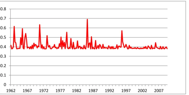
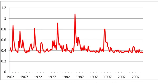
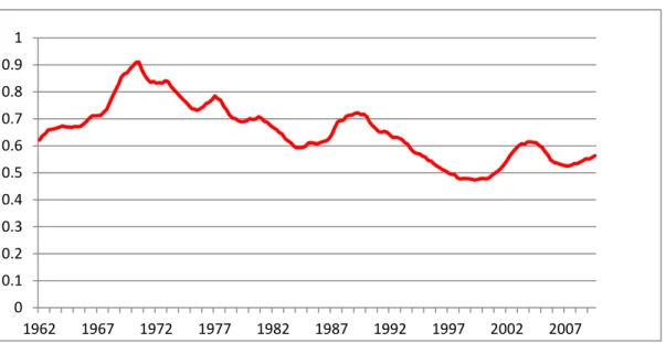
is relatively higher. Still, most of the series can be estimated with GARCH(1,1), and the residuals exhibit no serial correlation. Figures 1.1 - 1.5 report the consumption volatility series. The range of GARCH type models is 0.35 - 0.7% per quarter, consistent with the observed data. Consumption is more volatile during mid 1970’s, early 1980’s and early 1990’s, getting more stable after 1995. The GARCH and TGARCH series are relatively jagged, showing less clustering. The downward trend of EGARCH consumption series is very obvious. The HRS stochastic volatility series is very irregular during the first few years, and then smooth out later on. In contrast with GARCH models, both SV models predict a smooth transition of consumption volatility. However, the consumption volatility is slightly over-predicted. For instance, most of the time, the HRS quarterly volatility ranges from 0.8 to 1.2%.

The market volatility series can be found in Figures 2.1 - 2.5. The GARCH type and HRS SV models predict very jagged series. The market was more volatile during the mid 1970’s and early 2000’s. However, the HRS model significantly over-predicts market volatility. For instance, the market volatility in 1976 was almost 60%, defying the observed data. In contrast, the Durbin-Koopman SV series is overly smooth, and often, under-predicts market volatility. The poor performance can be reconciled by the fact that, SV series follows random walk pattern. It predicts change of volatility in infinitely short period of time. However, most quarterly series exhibits high persistence, which is better captured by GARCH type models. 5.2 Fama-MacBeth Style Regression

The unconditonal models can be consistently estimated by the cross-sectional regression method proposed by Black et al. (1972), General Method of Moments (GMM), and Fama and MacBeth (1973). We estimate equation (19) and its variants by the Fama-MacBeth (1973) approach. The first step is time series regression of each portfolio return against the BY premium and other scale factors. The second stage is cross-section regression for each quarter. The Fama-Macbeth estimates are simply the time average of cross-sectional estimates. Cochrane (1996) proves that if the betas do not vary over time and if the errors in the time series regression are cross-sectionally correlated but not correlated over time, the Fama-Macbeth estimate of risk price is identical to the pure cross-section OLS regression estimate. The Fama-Macbeth standard errors are identical to the cross-sectional standard errors, corrected for cross-sectional residual correlation.

Tables 1.1-1.5 report the Fama-MacBeth style regression results7. We compute the usual t statistics corrected for cross-section heteroskedasticity, Newey-West standard error, and then

(14)

both adjusted by the Shanken (1992) correction method8. The computed t-statistics turns out to be sensitive to the error correction method, rendering comparison difficult. The Shanken correction is directly related to the magnitude of each , coefficient estimate and inversely related to the factor volatility. The Shanken correction factor is larger when comparing to Lettau and Ludvigon’s (2002) results, due to low factor volatility. It should be noted that the standard CAPM predicts a zero intercept, but the models in this paper do not. It can be easily verified by equation (6). In fact, the intercepts () in most models are positive and significant.

Table 1.1 presents the traditional CAPM regression results corresponding to equation (19); and we see that the standard CAPM (first row) fails miserably. The R2 is only 0.055. Not only is the coefficient of risk premium insignificant, its sign (-0.8) is incorrect. However, Table 1.1 also shows that GARCH type and SV models show significant improvement. The model predicts a positive consumption volatility and negative market return volatility coefficient. Most of the conditional consumption volatility coefficients are significant after Shanken correction. For instance, the GARCH and TGARCH consumption volatility coefficients are significant even after adjusting for Newey-West and Shanken correction error. Our result, is by large consistent with the model prediction. Athough no conditional market volatility coefficient is significant, Table 2.1 shows that the conditional consumption and market volatility coefficients are jointly significant. For GARCH, TGARCH and HRS, the BY conditional equity premium are jointly significant after Newey-West and Shanken correction.

Following Jagannathan and Wang (1996), and Lettau and Ludvigson (2001), 2

R is used as an informal and intuitive measure - which shows the fraction of the cross-sectional variation of average returns that can be explained by the model. The 2

R range is 0.14 - 0.55. The best fitting model is GARCH, with R2 equal to 0.55. TGARCH model prediction is similar, though 2

R is slightly lower, the size of coefficients are larger, and the market volatility coefficient is significant at  equal to 10%. The GARCH type models outperform the SV models in all cases. Coefficients of the former model are also more likely to be correct. It means that either stochastic consumption volatility fails to explain equity premium, or that stochastic volatility fails to capture trending behavior in low frequency data. While quarterly data in general exhibits trend behavior, high-frequency data do not. Stochastic volatility is usually modelled to mimic return change in an infinitely small time horizon, which is believed to be trendless. Hence, GARCH type models are able to capture the trend behavior of quarterly time series.

The Fama and French (1993) result is replicated in Table 1.2 (corresponding to equation

(15)

(20)). We find that R2 is around 80%; the intercept and HML are significant-which are the same as Lettau and Ludvigosn (2002) and Fama and French (1993). However, by using data over a longer period, the sign of risk premium is no longer correct. When replacing market premium with consumption and market volatility, the same pattern is observed. After adjusting for small sample bias, HML coefficient is still significant, but the sign of consumption volatility is incorrect. The coefficient of EGARCH and Durbin-Koopman consumption coefficients are significant at  equal to 10%. More importantly, all GARCH and SV models slightly outperform the standard Fama-French model. The R2 of EGARCH is 0.84, 5% higher than that of Fama-French. Table 2.2 reports the joint significance test results. In all cases (except TGARCH), the null hypothesis is rejected.

Lettau and Ludvigson (2001) argue that including and its interaction with risk premium does not improve predictive power of their model. The same result is replicated in Table 1.3 with longer span of data. The R2 is 0.06 when the scale factor interact with market return. All coefficients are insignificant after adjusting for small sample error. However, this model performance is greatly improved once using the BY equity preimum. In the GARCH case, both conditional consumption and market volatility coefficients are significant. TheR2 is 0.62.

Table 1.4 shows that the forecasting variable fails to capture cross-sectional returns difference. The R2 is as low as 0.08 and the sign of market return coefficient remains incorrect. After using the BY theoretical conditional preimum, the model performance is significantly improved. We find that the coefficient signs of GARCH models are all correct. An interesting finding is that EGARCH model performance is greatly enhanced, once enters the equation as a separate variable. The 2

R of EGARCH is as high as 74%, increasing three-fold when compared to Table 1.3.

The full Lettau and Ludvigson scaled factor model results are reproduced in Table 1.5 (first row) using more recent data, in which the model is augmented with labor income growth and its interaction with . The 2

R is as high as 0.71, and further increases once market premium is replaced by consumption and market return volatilities. Most of the coefficients have the correct sign. The consumption and market volatility coefficients of EGARCH are individually and jointly significant after adjusting for Shanken correction. The

2

R (0.85) is highest among all regression models in this paper. Therefore, it can be concluded that EGARCH is the best fitting model in this paper. One plausible explanation is that the declining EGARCH consumption volatility is consistent with declining equity premium in recent decades. Hence, while Bansal and Yaron (2004) explain the declining premium by calibration, we provide statistical evidence to support their claim.

In Lettau and Ludvigson (2001) analysis, they fail to show significance of - a factor that the authors claim that would summarize future investment opportunity. They show that

(16)

However, if the BY theoretical equity premium is true, it should render these instruments redendent. In another word, when a consistent estimator of the conditional equity premium is available, the instrumental variables will not be necessary.

Table 2.3 reports the joint hypothesis testing of Lettau and Ludvigson (2001) instrumental variables( interacting with conditional consumption and market volatilities), corresponding to tables 1.3-1.5. For instance, the first column of table 1.3 is a joint test of sixth and seventh columns of table 1.3. The 2 statistics are corrected for cross-section heteroskedasticity, Newey-Wesley standard error, and then adjusted both for Shanken correction. The 5% critical value is 5.99. The first column corresponds to the 2 statistics of joint hypothesis testing of table 1.3 using various GARCH and SV models. The second and third columns are those of table 1.4 and 1.5, respectively. Clearly, Table 2.3 shows that, in all cases, once the standard error is corrected by Shanken method, no instrumental variables are significant. This result lends support to conditional consumption and market volatility as a reliable measure of conditional risk premium.

6. Discussion

An optimization-based regression model is estimated in this paper. We propose estimating the conditional equity premium directly by conditional consumption and market return volatilities. Most of the coefficient signs are correct. If 2

R is used as criteria, the volatility models outperform standard, CAPM. The EGARCH model, once augmented with Lettau and Ludvigson’s (2002) scaled factor, outperforms other models. In various 2

tests, it is shown that the theoretical premium renders all instrumental variables redundent, providing support for the BY model.

This study is different from the current research on the Bansal and Yaron (2004) models that those papers attempt to estimate some of the parameters in the general equilibrium model. For instance, Constantinides and Ghosh (2011) estimate the intertemporal elastcity of substitution from the Bansal and Yaron (2004) Euler equation using aggregate U.S consumption and dividend growth from 1931-2009. The original Bansal and Yaron (2004) Euler equation is a function of two unobservable latent state variables. Through some form of affine transformation, Constantinides and Ghosh (2011) show that the Euler equation is a function of observale aggregate log price-dividend ratio and log risk free rate. The key finding is that the Bansal and Yaron (2004) model requires higher consumption and dividend growth persistence than the observed data. Bansal et al. (2012) found supporting evidence for

(17)

the Long-Run Risks (LRR) model – a variant of Bansal and Yaron (2004). Using annual consumption and asset price data from 1930-2008, the authors find that the first and second calibrated moments match strongly to the actual U.S data; even the lower order autocorrelations fall insider the confidence band. However, Marakani (2009) demonstrates that, by variance ratios test, the LRR model implications are inconsistent with post-1929 U.S data. He contends that early studies fail to address the time aggregation bias inherent in the data. Other related empirical studies include Colacito and Croce (2011), Hansen et al. (2008), and Bansal et al. (2012). In essence, the above analyses are still calibration.

We provide a simple direct statistical method to test the validity of the BY model which depends on the parameter significance and coefficient of variation. In order to faciliate comparison with the existing studies, we are using the U.S data. An alternative to the Fama-MacBeth method is the GMM. However, we are estimating a linear factor model instead of the nonlinear Euler equations; and the potential estimation error has been adjusted by Shanken and Newey-West correction; we believe that there might not be too much efficiency gain from GMM

There are three limitations of this study. 1. Robustness remains as an issue. Lettau and Ludvigson (2001) fail to justify why only interacting labor income growth can explain return differences; we need a justification to explain why the EGARCH model performance greatly enhance once is introduced. 2. While there is a large literature comparing the preditive power of GARCH to SV models, to our knowledge, there is little comparison of these two models as explanatory variables. 3. The conditional volatilities are generated series that even the Shanken and Newey-West correction do not make adjustment for this estimation error. The standard error reported in section 5.2 can at best be regarded as a lower bound.

Current empirical studies of the Bansal and Yaron (2004) LRR models focus on calibration using U.S data. Future research can test the model validity by adopting statistical approach like this paper and using international data.

References

Bansal, R., Yaron, A., 2004. Risks for Long-Run: A Potential Resolution of Asset Pricing Puzzles. Journal of Finance. 59, 1481-1509.

Bansal, R., Kiku, D., Yaron, A., 2012. An Empirical Evaluation of the Long-Run risks Model for Asset Prices. Critical Finance Review. 1, 183-221.

(18)

Bansal, R., Kiku, D., Shaliastovich, I., Yaron, A, 2012. Volatility, the Macroeconomy and Asset Prices. National Bureau of Economic Research Working Paper: 18104.

Banz, R., 1981. The Relation between Return and Market Value of Common Stocks. Journal of Financial Economics. 9, 3-18.

Black, F., Jensen, M, C., Scholes, M., 1972. The capital asset pricing modeL Some empirical tests, in: Jensen, M. (Eds.), Studies in the Theory of Capital Markets. Pareger, New York, pp. 79-121.

Bollerslev, T., Chou, R., Kroner, K., 1992. ARCH Modeling in Finance: A Review of the Theory and Empirical Evidence. Journal of Econometrics. 52, 5-59.

Bollerslev, T., Engle, R., Nelson, D., 1994. Arch Models, in Engle, R., McFadden, D. (Eds.), Handbook of Econometrics, Volume 4. Elsevier Science, Amsterdam, pp. 2959-3038.

Campbell, J.Y., 1991. A Variance Decomposition for Stock Returns. Economic Journal. 101, 157-79.

Campbell, J., Shiller, R., 1988. The Dividend-Price Ratio and Expectations of Future Dividends and Discount Factors. Review of Financial Studies. 1, 195-227.

Chen, N., Roll, R., Ross, S., 1986. Economic Forces and the Stock Market. The Journal of Business. 59, 383-404.

Cochrane, J., 1996. A Cross-Sectional Test of Investment-Based Asset Pricing Model. Journal of Political Economy. 104, 572-621.

Colacito, R., Croce, M., 2011. Risks for the Long Run and the Real Exchange Rate. Journal of Political Economy. 119, 153-181.

Constantinides, G., Ghosh, A., 2011. Asset Pricing Tests with Long Run Risks in Consumption Growth. Review of Asset Pricing Studies. 1, 96-136.

Durbin, J., Koopman, S., 1997. Monte Carlo Maximum Likelihood Estimation of Non-Gaussian State Space Model. Biometrika. 84, 669-84.

(19)

Journal of Financial Economics. 33, 3-56.

Fama, E., MacBeth, J., 1973. Risk, Return and Equilibrium: Empirical Tests. Journal of Political Economy. 81, 607-36.

Fleming, J., Kirby, C., 2003. A Closer look at the Relation between GARCH and Stochastic Autoregressive Volatility. Journal of Financial Econometrics. 1, 356-419.

Ghysels, E., Harvey, A., Renault, E, 1996. Stochastic Volatility, in: Maddala, G., Rao, C. (Eds.), Handbook of Statistics, Volume 14, Statistical Methods in Finance. North-Holland, Amsterdam, pp: 119-191.

Hansen, L., Heaton, K., Li, N., 2008. Consumption Strikes Back? Measuring Long Run Risk. Journal of Political Economy. 116, 260-302.

Hansen, L., Singleton, K., 1982. Generalized Instrumental Variables Estimation of Nonlinear Rational Expectations Models. Econometrica. 50, 1269-86.

Harvey, A., Ruiz, E., Shephard, N., 1994. Multivariate Stochastic Variance Models. Review of Economic Studies. 61, 247-64.

Heynen, R., Kat, H., 1994. Volatility Prediction: A Comparison of the Stochastic Volatility, GARCH (1,1) and EGARCH (1,1) Models. Journal of Derivative. 2, 50-65.

Hull, J., White, A., 1987. The Pricing of Option on Assets with Stochastic Volatilities. Journal of Finance. 42, 281-300.

Jagannathan, R., Wang Z., 1996. The Conditional CAPM and the Cross-Section of Expected Returns. The Journal of Finance. 51, 3-53.

Lamont O., 1998. Earnings and Expected Returns. Journal of Finance. 53, 1563-87.

Lettau, M. Ludvigson, S., 2001. Resurrecting (C)CAPM: A Cross-Sectional Test When Risk Premia are Time-Varying. Journal of Political Economy. 109, 1238-1287.

Marakani, S., 2009. A long-Run Consumption Risks: Are They There? City University of Hong Kong Working Paper.

(20)

Preminger, A., Haftner, C., 2006. Deciding between GARCH and Stocastic Volatility Via Strong Decision Rules. Monaster Center of Economic Research, Ben Gurion University of the Negev, working paper no. 06-03.

Roll, R., 1977. A Critique of the Asset Pricing Theory’s Test: Part 1: On Past and Potential Testability of the Theory. Journal of Financial Economics. 4, 129-76.

Shanken, J., 1992. On the Estimation of Beta-Pricing Models. Review of Financial Studies. 5, 1-34.

Taylor, S., 1999. Modeling Stochastic Volatility: A Review and Comparative Study. Mathematical Finance. 4, 183-204.

(21)

Appendix

Figure 1.1 Estimated GARCH Consumption (Quarterly) Volatility

Source: The (log) consumption growth data are available from Ludvigson and Lettau’s website -http://www.econ.nyu.edu/user/ludvigsons/. The first-differenced time series is used as input for a GARCH(1,1) process.

Figure 1.2 Estimated EGARCH Consumption (Quarterly) Volatility

Source: The (log) consumption growth data are available from Ludvigson and Lettau’s website -http://www.econ.nyu.edu/user/ludvigsons/. The first-differenced time series is used as input for a EGARCH(1,1) process.

0 0.1 0.2 0.3 0.4 0.5 0.6 0.7 0.8 1962 1967 1972 1977 1982 1987 1992 1997 2002 2007 0 0.05 0.1 0.15 0.2 0.25 0.3 0.35 0.4 0.45 0.5 1962 1967 1972 1977 1982 1987 1992 1997 2002 2007

(22)

Figure 1.3 Estimated TGARCH Consumption (Quarterly) Volatility

Source: The (log) consumption growth data are available from Ludvigson and Lettau’s website -http://www.econ.nyu.edu/user/ludvigsons/. The first-differenced time series is used as input for a TGARCH(1,1) process.

Figure 1.4 Estimated Stochastic (Harvey, Ruiz and Shephard, 1994) Consumption (Quarterly) Volatility

Source: The (log) consumption growth data are available from Ludvigson and Lettau’s website -http://www.econ.nyu.edu/user/ludvigsons/. The first-differenced time series is used as input and estimated by the Harvey, Ruiz and Shephard (1994) process.

0 0.2 0.4 0.6 0.8 1 1.2 1962 1967 1972 1977 1982 1987 1992 1997 2002 2007 0 0.2 0.4 0.6 0.8 1 1.2 1.4 1.6 1.8 2 1962 1967 1972 1977 1982 1987 1992 1997 2002 2007

(23)

Figure 1.5 Estimated Stochastic (Durbin and Koopman, 1997) Consumption (Quarterly) Volatility

Source: The (log) consumption growth data are available from Ludvigson and Lettau’s website -http://www.econ.nyu.edu/user/ludvigsons/. The first-differenced time series is used as input and estimated by the Durin and Koopman (1997) process.

0 0.1 0.2 0.3 0.4 0.5 0.6 0.7 0.8 0.9 1 1962 1967 1972 1977 1982 1987 1992 1997 2002 2007

(24)

Figure 2.1 Estimated GARCH Market (Quarterly) Volatility

Source: The U.S Market data are available from Fama’s website - http://mba.tuck.dartmouth.edu/pages/faculty/ken.french/data_library.html. The first-differenced time series is used as input for a GARCH(1,1) process.

Figure 2.2 Estimated EGARCH Market (Quarterly) Volatility

Source: The U.S Market data are available from Fama’s website - http://mba.tuck.dartmouth.edu/pages/faculty/ken.french/data_library.html.

The first-differenced time series is used as input for a EGARCH(1,1) process.

0 2 4 6 8 10 12 14 16 1962 1967 1972 1977 1982 1987 1992 1997 2002 2007 0 2 4 6 8 10 12 14 16 18 1962 1967 1972 1977 1982 1987 1992 1997 2002 2007

(25)

Figure 2.3 Estimated TGARCH Consumption (Quarterly) Volatility

The first-differenced time series is used as input for a TGARCH(1,1) process.

Figure 2.4 Estimated Stochastic (Harvey, Ruiz and Shephard, 1994) Market (Quarterly) Volatility

The first-differenced time series is used as input and estimated by the Harvey, Ruiz and Shephard (1994) process.

0 5 10 15 20 25 1962 1967 1972 1977 1982 1987 1992 1997 2002 2007 0 10 20 30 40 50 60 70 1962 1967 1972 1977 1982 1987 1992 1997 2002 2007

(26)

Figure 2.5 Estimated Stochastic (Durbin and Koopman, 1997) Market (Quarterly) Volatility

The first-differenced time series is used as input and estimated by the Durin and Koopman (1997) process.

0 2 4 6 8 10 12 1962 1967 1972 1977 1982 1987 1992 1997 2002 2007

(27)

Table 1.1 Fama-MacBeth Regressions using 25 Fama-French Portfolios:

CAPM

Volatility Model Intercept c2,t1

2 1 t , m   Rvm R 2 Coefficient 4.4 -0.8 0.055 T-value (5.85)* (-1.18) (5.82)# (-0.87) (4.96)+ (-0.74) (4.93)& (-0.64) GARCH Coefficient 3.53 0.094 -0.72 0.55 T-value (7.33) (8.4) (-2.6) (3.23) (3.7) (-1.3) (5.85) (3.87) (-1.57) (2.6) (1.78 (-0.69) EGARCH Coefficient 4.06 -0.02 -0.63 0.14 T-value (9.08) (-0.69) ( -1.68) (8.08) (-0.61) (-1.44) (6.9) (-1.42) (-1.14) (6.14) (-1.21) (-.1.0) TGARCH Coefficient 3.75 0.14 -1.94 0.54 T-value (8.68) (5.78) (-3.49) (4.52) (2.97) (-1.8) (6.84) (3.81) (-2.28) (3.56) (1.75) (-1.18) HRS Coefficient 3.13 -0.26 4.0 0.21 T-value (15.44) (-2.13) (1.55) (9.72) (-1.34) (0.97) (5.13) (-2.94) (0.85) (3.24) (-1.85) (0.54) DK Coefficient 3.6 0.055 1.62 0.2 T-value (26.93) (0.76) (2.72) (16.1) (0.45) (1.62) (5.09) (1.33) (2.53) (3.04) (0.79) (1.51)

(28)

2 1 t , c 

 and 2_m_,_t_₁ are the estimated conditional consumption and market volatilities respectively. R_vm is the value-weighted U.S. market return;

* t statistics adjusted for cross-section heteroskedasticiy;

#

adjusted for heteroskedasticiy and Shanken correction;

+

Newey-West adjusted standard error;

&

(29)

Table 1.2 Fama-MacBeth Regressions using 25 Fama-French Portfolios:

Fama-French Factors

Volatility Model Intercept 2 1 t , c   2 1 t , m   R_vm SMB HML 2 R Coefficient 4.02 -1.19 0.61 1.33 0.79 T-value (4.23)* (-1.28) (3.59) (7.04) (4.05)# (-1.04) (1.38) (2.97) (3.82)+ (-0.98) (1.47) (3.23) (3.65)& (-0.84) (1.03) (2.26) GARCH Coefficient 3.59 -0.014 -0.45 0.65 1.29 0.8 T-value (9.65) (-0.97) (-1.43) (4.18) (7.49) (8.4) (-0.83) (-1.2) (1.5) (2.9) (6.86) (-1.03) (-1.49) (1.56) (3.14) (5.98) (-0.88) (-1.26) (1.04) (2.08) EGARCH Coefficient 3.04 -0.04 -0.28 0.67 1.26 0.84 T-value (13.48) (-2.3) (-0.79) (5.5) (8.63) (11.3) (-1.88) (-0.64) (1.6) (2.8) (5.84) (-3.04) (-0.65) (1.63) (3.04) (4.88) (-2.47) (-0.53) (1.05) (1.96) TGARCH Coefficient 3.31 -0.03 -0.31 0.62 1.31 0.79 T-value (12.8) (-0.71) (-0.51) (3.8) (6.76) (11.5) (-0.64) (-0.45) (1.4) (2.9) (6.74) (-0.9) (-0.49) (1.51) (3.17) (6.19) (-0.81) (-0.44) (1.03) (2.17) HRS Coefficient 3.05 -0.08 -1.97 0.64 1.33 0.81 T-value (15.0) (-1.03) (-0.67) (4.27) (7.33) (13.2) (-0.9) (-0.6) (1.5) (2.9) (5.54) (-1.49) (-1.09) (1.56) (3.23) (4.87) (-1.27) (-0.92) (1.04) (2.16) DK Coefficient 3.06 -0.05 -0.33 0.69 1.3 0.82 T-value (15.45) (-1.57) (-0.74) (4.72) (7.86) (13.0) (-1.3) (-0.6) (1.6) (2.9) (5.65) (-2.29) (-0.9) (1.71) (3.16) (4.74) (-1.85) (-0.74) (1.1) (2.05)

(30)

2 1 t , c 

#

+

&

(31)

Table 1.3 Fama-MacBeth Regressions using 25 Fama-French Portfolios:

CAPM with

as Instrument

Volatility Model Intercept 2 1 t , c   2 1 t , m   Rvm 2 1 t , c   2 1 t , m   Rvm R 2 Coefficient 4.72 -1.08 -0.13 0.06 T-value (2.78)* (-0.68) (-0.21) (2.7) # (-0.63) (-0.2) (6.13)+ (-1.14) (-0.46) (6.05)& (-0.95) (-0.43) GARCH Coefficient 4.1 0.08 -1.43 0.003 0.05 0.62 T-value (6.6) (6.19) (-2.86) (1.12) (1.03) (2.7) (2.5) (-1.17) (0.46) (0.42) (7.73) (3.95) (-4.0) (1.82) (1.52) (3.19) (1.65) (-1.64) (0.75) (0.62) EGARCH Coefficient 4.17 -0.043 -1.62 -0.0004 -0.03 0.25 T-value (5.01) (-1.32) (-1.92) (-0.13) (-0.52) (3.02) (-0.8) (-1.15) (-0.08) (-0.31) (6.96) (-3.31) (-3.15) (-0.34) (-1.07) (4.19) (-1.94) (-1.88) (-0.2) (-0.63) TGARCH Coefficient 3.7 0.1 -2.65 0.006 0.08 T-value (9.48) (2.25) (-3.46) (1.82) (1.56) (4.3) (1.03) (-1.57) (0.83) (0.7) (6.35) (1.99) (-4.15) (2.87) (2.04) (2.91) (0.91) (-1.89) (1.31) (0.93) HRS Coefficient 4.2 -0.08 6.88 -0.007 0.013 0.49 T-value (7.05) (-0.68) (3.78) (-1.17) (0.32) (4.4) (-0.42) (2.3) (-0.72) (0.19) (5.91) (-1.63) (1.78) (-1.71) (0.35) (3.67) (-0.99) (1.1) (-1.05) (0.22) DK Coefficient 3.83 0.07 1.52 -0.003 -0.03 0.23 T-value (13.29) (1.11) (2.49) (-0.63) (-0.62) (7.9) (0.66) (1.48) (-0.37) (-0.36) (6.06) (1.96) (2.93) (-1.27) (-0.03)

(32)

(3.6) (1.16) (1.73) (-0.74) (-0.62) 2 1 t , c 

#

+

&

(33)

Table 1.4 Fama-MacBeth Regressions using 25 Fama-French Portfolios:

CAPM with

and

as Instruments

Volatility Intercept _c2_,_t₁ 2m,t1 Rvm 2 1 t , c   2 1 t , m   R_vm 2 R Coefficient 4.75 -0.006 -1.08 -0.02 0.08 T-value (3.06) * (-0.8) (-0.74) (-0.36) (2.7) # _(-0.72) _(-0.62) _(-0.32) (6.16) + _(-1.47) (-1.14) (-0.75) (5.55) & _(-1.29) _(-0.89) _(-0.65) GARCH Coefficient 4.01 0.006 0.08 -1.4 0.0023 0.04 0.62 T-value (6.35) (1.02) (6.69) (-2.8) (0.97) (0.93) (2.76) (0.44) (2.9) (-1.2) (0.42) (0.4) (7.42) (1.64) (3.91) (-4.0) (1.56) (1.36) (3.22) (0.71) (1.59) (-1.73) (0.67) (0.59) EGARCH Coefficient 1.4 0.002 -0.03 -1.08 -0.0006 -0.02 0.74 T-value (3.1) (0.36) (-2.77) (-2.46) (-0.51) (-0.73) (1.35) (0.16) (-1.76) (-1.06) (-0.22) (-0.32) (2.06) (0.39) (-2.35) (-2.31) (-0.56) (-0.67) (0.9) (0.17) (-1.0) (-0.99) (-0.24) (-0.29) TGARCH Coefficient 3.06 0.005 0.008 -2.56 0.001 0.0004 0.73 T-value (7.59) (1.06) (1.19) (-4.21) (0.48) (0.01) (3.6) (0.5) (1.09) (-1.97) (0.23) (0.005) (5.19) (1.23) (1.22) (-4.08) (0.57) (0.01) (2.5) (0.58) (1.1) (-1.91) (0.27) (0.0052) HRS Coefficient 4.13 -0.007 -0.09 7.0 -0.007 0.01 0.49 T-value (4.14) (-1.11) (-0.66) (2.78) (-1.16) (0.27) (2.6) (-0.72) (-0.41) (1.71) (-0.68) (0.16) (5.59) (-1.66) (-1.64) (1.86) (-1.7) (0.32) (3.5) (-1.04) (1.15) (-1.02) (-1.0) (0.19) DK Coefficient 3.6 -0.015 0.056 1.33 -0.008 -0.08 0.32 T-value (13.14) (-2.09) (0.87) (2.24) (-1.85) (-1.67) (6.02) (-0.95) (0.4) (1.03) (-0.85) (-0.76) (6.03) (-2.69) (1.72) (2.71) (-2.0) (-2.16) (2.8) (-1.23) (0.78) (1.23) (-1.19) (-0.99)

(34)

2 1 t , c 

#

+

&

(35)

Table 1.4 Fama-MacBeth Regressions using 25 Fama-French Portfolios:

Ludvigson and Lettau’s Scaled Factor Model

Volatility Intercept 2_c_,_t₁ m2,t1 Rvm y 2 1 t , c   2 1 t , m   R_vm y 2 R Coefficient 6.6 -0.004 -3.64 0.01 -0.08 0.0002 0.71 T-value (9.47) * (-0.69) (-5.32) (2.56) (-2.81) (3.33) (3.7) # _(-0.27) _(-3.6) _(0.99) _(-1.08) _(1.3) (6.4) + (-1.11) (-3.11) (3.07) (-2.26) (3.89) (2.45) & _(-0.43) _(-1.18) _(1.19) _(-0.87) _(1.5) GARCH Coefficient 3.7 0.005 0.04 -1.3 0.003 0.002 0.033 0.0001 0.67 T-value (6.53) (0.83) (1.9) (-2.87) (0.76) (0.67) (0.64) (1.73) (3.3) (0.42) (0.96) (-1.45) (0.38) (0.34) (0.33) (0.88) (6.69) (1.36) (2.1) (-3.77) (1.37) (1.16) (1.03) (2.99) (3.4) (0.7) (1.06) (-1.9) (0.69) (0.58) (0.52) (1.51) EGARCH Coefficient 2.42 -0.005 -0.07 -1.46 -0.003 -0.002 -0.06 0.0000 8 0.85 T-value (5.19) (-0.89) (-5.2) (-4.35) (-0.78) (-0.98) (-1.5) (1.78) (2.22) (-0.38) (-2.2) (-1.84) (-0.33) (-0.42) (-0.67) (0.76) (3.68) (-1.32) (-4.17) (-2.71) (-1.06) (-1.48) (-1.97) (2.43) (1.57) (-0.56) (-1.76) (-1.15) (-0.45) (-0.63) (-0.84) (1.03) TGARCH Coefficient 3.06 0.004 -0.02 -2.58 0.002 0.0004 -0.013 0.0001 0.74 T-value (6.41) (0.55) (-0.33) (-4.23) (0.29) (0.14) (-0.25) (1.74) (2.96) (0.25) (-0.15) (-1.93) (0.14) (0.06) (-0.12) (0.8) (4.56) (0.88) (-0.48) (-3.59) (0.46) (0.2) (-0.37) (2.56) (2.1) (0.4) (-0.22) (-1.65) (0.21) (0.09) (-0.17) (1.17) HRS Coefficient 2.7 -0.006 -0.2 -0.52 0.003 -0.005 -0.03 0.0001 0.74 T-value (4.8) (-1.08) (-2.07) (-0.16) (1.64) (-0.9) (-0.69) (1.64) (2.16) (-0.55) (-1.04) (-0.08) (0.82) (-0.45) (-0.35) (0.82) (3.95) (-1.38) (-3.02) (-0.23) (1.26) (-1.27) (-0.63) (2.71) (2.0) (-0.69) (-1.51) (-0.11) (0.63) (-0.64) (-0.32) (1.36) DK Coefficient 2.4 -0.009 -0.004 1.06 0.011 -0.004 -0.04 0.0001 0.62 T-value (4.4) (-1.88) (-0.15) (2.41) (3.16) (-1.64) (-1.29) (3.2) (2.41) (-0.58) (-0.04) (0.8) (1.11) (-0.45) (-0.43) (0.84) (4.44) (-1.88) (-0.15) (2.41) (3.16) (-1.64) (-1.29) (3.2) (1.71) (-0.72) (-0.05) (0.92) (1.22) (-0.63) (-0.5) (1.2)

(36)

y

 denotes log labor income growth.

2 1 t , c 

 and 2_m_,_t_₁ are the estimated conditional consumption and market volatilities respectively. Rvm is the value-weighted U.S. market return;

#

+

&

(37)

Table 2.1 Fama-MacBeth Regressions using 25 Fama-French Portfolios

CAPM

Tests for Joint Significance

Volatility Model 2 1 ,t c  and _m2_,_t_₁ 99 . 5 2 c   GARCH 76.5* 14.6# 14.1+ 2.7& EGARCH 4.5 3.3 2.5 1.9 TGARCH 61.5 16.1 61.5 16.13 HRS 7.4 2.9 14.0 5.5 DK 7.7 2.7 7.4 2.6 2

 statistics for testing joint significance of 2_c_,_t_₁ and 2_m_,_t_₁ coefficient from Table 1.1. The critical value is 5.99.

#

+

&

(38)

Table 2.2 Fama-MacBeth Regressions using 25 Fama-French Portfolios

Fama French Factors

Tests for Joint Significance

Volatility Model c2,t1 and

2 1 ,t m  99 . 5 2 c   GARCH 2.60* 1.88# 3.54+ 2.52& EGARCH 7.6 4.9 9.65 6.12 TGARCH 0.93 0.74 0.95 0.77 HRS 1.25 0.95 3.01 2.2 DK 2.5 1.69 5.23 3.43 2

 statistics for testing joint significance of 2_c_,_t_₁ and 2_m_,_t_₁ coefficient from Table 1.2. The critical value is 5.99.

#

+

&

(39)

Table 2.3 Fama-MacBeth Regressions using 25 Fama-French Portfolios

CAPM with as Instrument

CAPM with and

as Instruments

Ludvigson and

Lettau’s Scaled Factor Model Volatility Model (Table 1.3) (Table 1.4) (Table 1.5) GARCH 1.68* 0.99 0.45 0.3# 0.19 0.13 6.87+ 3.8 1.9 1.15# 0.7 0.47 EGARCH 8.01 1.57 23.6 2.8 0.28 4.17 7.34 0.6 6.94 2.6 0.11 1.25 TGARCH 4.05 3.9 3.89 0.85 0.86 0.82 18.15 5.6 7.2 3.77 1.23 1.5 HRS 3.4 0.68 0.8 1.28 0.26 0.2 5.43 3.22 1.78 2.05 1.19 0.45 DK 0.4 2.78 1.4 0.14 0.58 0.2 1.78 5.02 3.88 0.62 1.05 0.57 2

 statistics for testing joint significance of ∙ 2 1 t , c   and ∙ 2 1 t , m   coefficient for Tables 1.3-1.5. The critical value is 5.9.

#

+

&