NCER Working Paper Series
Does implied volatility reflect a wider information set than econometric forecasts?
Ralf Becker, Adam E. Clements and James Curchin Working Paper #15
Does implied volatility reflect a wider information set than
econometric forecasts?
Ralf Becker
#, Adam E. Clements
∗and James Curchin
*#
Economic Studies, School of Social Sciences, University of Manchester, ∗
School of Economics and Finance, Queensland University of Technology
Corresponding author
Adam Clements
School of Economics and Finance Queensland University of Technology GPO Box 2434, Brisbane Q, Australia 4001 email [email protected]
Ph +61 7 3138 2525, Fax +61 7 3138 1500.
Abstract
Much research has addressed the relative performance of option implied volatilities and econometric model based forecasts in terms of forecasting asset return volatility. The general theme to come from this body of work is that implied volatility is a superior forecast. Some authors attribute this to the fact that option markets use a wider information set when forming their forecasts of volatility. This article considers this issue and determines whether S&P 500 implied volatility reflects a set of economic information beyond its impact on the prevailing level of volatility. It is found, that while the implied volatility subsumes this information, as do model based forecasts, this is only due to its impact on the current or prevailing level of volatility. Therefore, it appears as though implied volatility does not reflect a wider information set than model based forecasts, implying that implied volatility forecasts simply reflect volatility persistence in much the same way of as do econometric models.
Keywords: Implied volatility, VIX, volatility forecasts, informational efficiency.
JEL Classification: C12, C22, G00, G14
Acknowledgements: The authors thank Adrian Pagan whose comments on related work motivated the current research, Stan Hurn for constructive feedback on earlier versions of the article and seminar participants at the Queensland University of Technology
1 Introduction
The behaviour of option implied volatilities have attracted a great deal of research attention. Both the relative forecast accuracy and informational efficiency of implied volatilities (IV) have been considered by numerous authors.
Fleming (1998), Jiang and Tian (2003) and Becker, Clements and White (2006), amongst others have examined whether various IV measures subsume historical information (predominantly return data) commonly used when forecasting volatility. While Fleming (1998) and Jiang and Tian (2003) find that IV is efficient with respect to such information, Becker, Clements and White (2006) find that S&P 500 IV does not completely subsume a diverse set of information including model based forecasts (MBF).
Poon and Granger (2003, 2005) provide wide ranging surveys of articles comparing various forecasting approaches. The general pattern revealed by Poon and Granger (2003, 2005) is that option based IV produce superior forecasts of volatility relative to competing MBF. Poon and Granger (2003) state that this general result is of little surprise as IV forecasts are based on a larger and timelier information set.
This study addresses the issue of whether IV forecasts are in fact based on a wider information set than MBF. We consider if non-return, economic information influences IV forecasts beyond its impact on current levels of volatility. In doing so, we highlight whether option markets utilize economic information to generate forecasts that reflect more than persistence in volatility which MBF capture. In this context, the information considered is interest rate and commodity price data, information that traditionally is incorporated into time series models of volatility. This information has been selected as it would influence option market participants’ expectations of future equity volatility.
We begin by determining whether IV forecasts and MBF subsume the chosen set of non-return information. To do so, a similar approach to the informational efficiency studies discussed above is taken. To ensure the validity of the results from this first stage, it is also necessary to check whether the forecasts themselves are related to the non-return information. However, to determine if the economic information influences IV forecasts beyond its impact on current levels of volatility, and hence if IV reflects more than just volatility persistence, we need to delve deeper. Next we examine whether economic information is reflected in current levels of volatility and forecasts of changes from the current level of volatility. If the economic information is found to be relevant to the current level of volatility, and a forecast is found to subsume this information, but it is not related to forecasts of the change in the level of volatility, then one can conclude that a forecast does not reflect the information beyond its impact on current levels of volatility. It is found that while IV does subsume such non-return information, as do MBF, it is only through its impact on current levels of volatility. Given this result, it appears as IV does not reflect a wider information set than standard MBF, indicating that IV expectations simply reflect volatility persistence.
This paper proceeds as follows. Section 2 presents the data relevant to this study. Section 3 outlines the methodology utilized to address the research question at hand. Sections 4 and 5 present the empirical results and concluding comments respectively.
2 Data
To address the research question at hand four different sets of data are required. Equity returns, an estimate of IV, realisations of equity volatility and the economic style data, specifically term structure and commodity prices are utilized here. Each set of data will now be discussed in turn.
The study is based on daily S&P 500 index returns, from 2 January 1990 to 17 October 2003 (3481 daily observations). The implied volatility measure utilized here is that provided by the Chicago Board of Options Exchange, the VIX1. The VIX is an implied volatility index derived from a number of put and call options on the S&P 500 index, which generally have strike prices close to the current index value with maturities close to the target of 22 trading days2. It is derived without reference to a restrictive option pricing model. For technical details relating to the construction of the VIX index, see Chicago Board of Options Exchange (2003). After allowing for a potential volatility risk premium, the VIX is constructed to be a general measure of the market's estimate of average S&P 500 volatility over the subsequent 22 trading days (Blair, Poon and Taylor 2001, and Christensen and Prabhala, 1998)3. As highlighted by Jiang and Tian (2003), the advantages of such a model-free approach to computing implied volatility are two-fold4. Relative to a model-based estimate such as Black-Scholes, a model-free estimate incorporates more information from a range of observed option prices. In the current context, utilising model-free estimates avoids a joint test of both the option pricing model and market efficiency.
The measure of actual volatility used here is realised volatility (RV), constructed from intra-day S&P 500 index data (see Andersen, Bollerlsev, Diebold and Labys 2001, 2003 for a discussion of RV)5. In dealing with practical issues such as intra-day seasonality and sampling frequency when constructing daily RVt, the signature plot methodology of Andersen et al. (1999) is followed. Given this approach, daily RVt estimates are constructed using 30 minute S&P 500 index returns.
The set of economic (non-return) information comprises of variables that can be reasonably assumed to be related to general economic conditions and equity market performance and volatility. The variables are the slope of the term structure
represented by the difference between one and ten year US Treasury bond yields (slope), the credit spread between BBB rated commercial paper and US Treasury bills (cspr), absolute daily oil price change (oil), and an indicator variable (doil) which is unity when the change in oil price is positive and zero when the change in oil price is negative. While this is by no means an exhaustive list of economic variables, they relate to changes in the level of economic activity (cspr), inflationary expectations (slope) and the headline commodity price in terms of oil, which impacts on the cost
1
The VIX index used here is the most recent version of the index, introduced on September 22, 2003. VIX data for this study was downloaded from the CBOE website.
2
The daily volatility implied by the VIX can be calculated when recognising that the VIX quote is equivalent to 100 times the annualised return standard deviation. Hence (VIX/(100 252))2
represents the daily volatility measure (see CBOE, 2003).
3
Quoting from the CBOE White paper (2003) on the VIX, "VIX [...] provide[s] a minute-by-minute snapshot of expected stock market volatility over the next 30 calendar days."
4
They utilise a different approach to that embodied into the calculation of the VIX.
5
incurred by many firms and individuals, and thus inflation. These are also variables that are available at the daily frequency. The information considered is of a wider nature than that traditionally incorporated in MBF.
3 Methodology
We begin by describing the set of models upon which MBF are based. These are selected from a range of different model classes frequently applied in the financial econometrics literature. The chosen MBF are the GARCH(1,1) (gar), an asymmetric GARCH-type GJR model (gjr), a stochastic volatility (sv) model, two time-series models of RV a short memory (arma) and long memory (arfima). These models are also extended by the inclusion of RV as an additional explanatory variable (garrv, gjrrv, and svrv)6. As the VIX is designed as a fixed 22 day ahead forecast, each of the models are used to produce forecasts of average 22 day ahead volatility. Forecasts are based on parameters estimated recursively from a rolling window of 1000 observations. This procedure results in 2460 22 day ahead forecasts.
The first step in the methodology is to test whether these forecasts subsume the selected economic information. To do so, the testing strategy employed by Fleming (1998) and Becker, Clements and White (2006) is used. This entails testing whether the forecast errors given a volatility forecast (using both VIX and MBF discussed above, denoted below with superscripts) are orthogonal to a set of available information, zt. In this instance, the information set z t contains the economic data outlined above and the target to be forecast is realized volatility observed over the ensuing 22 trading days, RVt+1→t+22. Therefore the forecast errors are defined as
) ( 1 22 22 1→+ +→+ + − + = t t t t t RV α β f ε (1)
where ft+1→t+22 is a 22 day ahead volatility forecast based on either the VIX or MBF ( fVIXt+1→t+22 or f MBFt+1→t+22). The incorporation of the parameters, αand β are is
motivated by traditional volatility forecast regressions as not all forecasts will be entirely unbiased. When considering the VIX as a potential volatility forecast, the inclusion of an intercept allows for a potential volatility risk premium in the VIX. If the sequence of zero-mean forecast errors
{ }
εˆ are unrelated to any other conditioning t information, then the selected forecast subsumes that information. In this instance, two sets of analyses will be conducted using both fVIXt+1→t+22 and fMBFt+1→t+22.A direct way of testing the orthogonality of
{ }
εˆ is proposed by Fleming (1998), t and used by Becker, Clements and White (2006), which employs the Generalized Method of Moments (GMM) framework. Parameter estimates of equation (1) are obtained by minimising V =g(α,β)'Hg(α,β), where∑
= +→+ + → + − − = T t t t t t t f z RV T g 1 22 1 22 1 ' ) ( 1 ) , (α β α β (2) with zt being the selected set of instruments including the economic variables to which the forecast errors are hypothesised to be orthogonal. The weighting matrix His chosen to be the variance-covariance matrix of the moment conditions in g(α,β), where allowance is made for residual correlation (see Hansen and Hodrick, 1980).
6
The traditional test of overidentifying restrictions in the GMM framework is then a test of whether the VIX, MBF, or both subsume the non-return economic information.
Two sets of tests using (2) will be conducted, using both fVIXt+1→t+22 and
} , , , , , , , { 22
1 gar gjr sv garrv gjrrv svrv arma arfima
f MBFt+→t+ = , in this instance β will
be a vector of parameters. This will require two sets of instruments,
{
f slope cspr oil doil}
z VIXt t VIX t 1, 1 22, , , , ) ( + → + = and
{
f slope cspr oil doil}
z MBFt t MBF t 1, 1 22, , , , ) ( + → +
= . It is necessary to have the independent
variables included in the set of instruments to ensure that RVt+1→t+22−α−β ft+1→t+22
is a forecast error, and thus testing its correlation with z t tests whether the forecast in question subsumes the information in zt.
To ensure that any conclusions from this first step are valid, it is then necessary to check whether the chosen instruments are related to the various volatility forecasts. This is important because if it were found that the various forecasts errors were uncorrelated with the instruments, this could be due to one of two reasons. The forecasts do in fact subsume the selected set of instruments or the instruments are entirely unrelated to the forecasts. Thus, to eliminate the second possibility and draw clear conclusions regarding the research question at hand,
∑
= +→+ − = T t t t t z f T g 1 22 1 ) ( 1 ) , (α β α (3)is estimated with zt =
{
1,slope,cspr,oil,doil}
. The test for overidentifying restrictions will be used to gauge whether the instruments are correlated with the forecasts, that is they are relevant variables in relation to the volatility forecasts.Upon ascertaining whether the forecasts, IV and MBF subsume the information in zt, we now examine if this is simply due to the impact of zt on the current level of volatility, RVt. We begin by testing the relationship between zt using the same GMM framework as discussed above,
∑
= − = T t t t z RV T g 1 ) ( 1 ) , (α β α , (4)which is estimated with zt =
{
1,slope,cspr,oil,doil}
. The test for overidentifyingrestrictions will be used to gauge whether the instruments are correlated with the prevailing level of volatility. Empirical results will be reported for a number of moving averages of RVt. To reveal whether forecasts of the changes in volatility reflect the non-return information,
∑
= +→+ − − = T t t t t t RV z f T g 1 22 1 ) ( 1 ) , (α β α . (5)is estimated. Once again, zt =
{
1,slope,cspr,oil,doil}
and the test for overidentifyingrestrictions will reveal whether the instruments are correlated with the forecast changes in volatility.
4 Results
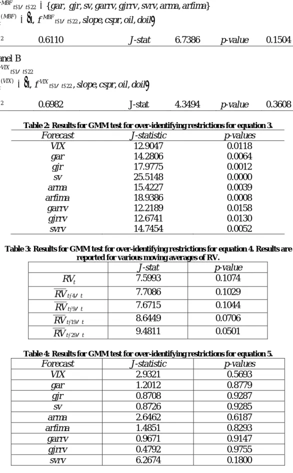
Table 1 provides the GMM results for the test for over-identifying restrictions for equation (2) given both fVIXt+1→t+22 and fMBFt+1→t+22. Recall, that results of these
tests are indicative of whether the selected forecast (or set of forecasts) subsume the information represented by the instruments. Panel A of Table 1 reports the result for the MBF while Panel B does so for the VIX.
INSERT TABLE 1 ABOUT HERE
We will begin by considering the MBF result in Panel A. The reported R2
indicates that the selected combination of MBF explains a significant proportion of the variation in future realizations of RV, RVt+1→t+22. The reported J-statistic (~# of
moments - # of parameters) of 6.7386 represents a p-value of 0.1504. Therefore, we would not reject the null hypothesis that forecast errors from the combination of MBF are orthogonal to the information contained in zt, and thus indicating that these MBF may subsume the selected economic variables.
Turning to Panel B, the results for the VIX paint a similar picture. The reported
2
R indicates that the VIX explains slightly more of the variation in RVt+1→t+22 than
the combination of MBF. The J-statistic of 4.3494 and an associated p-value of 0.3608 shows that VIX forecast errors are orthogonal to the information in zt and thus may also subsume this information.
INSERT TABLE 2 ABOUT HERE
Table 2 contains the over-identifying restriction test results, J-statistics and associated p-values for equation (3). These results show whether the instruments are correlated with the forecasts, highlighting whether they are in fact relevant for forecasting volatility. For all forecasts the null hypothesis of no correlation can be rejected at a 5% significance level, with the two largest p-values being just greater than 1%. These results, combined with those reported in Table 1 reveal that all of the forecasts, VIX and MBF do subsume the selected economic information. We now turn to the issue of whether this is due simply to the impact of the economic variables on prevailing volatility, or whether the VIX forecast simply reflects volatility persistence.
INSERT TABLE 3 ABOUT HERE
Table 3 reports the results for equation 4, indicating whether prevailing volatility is related to the selected set of instruments. Results are reported for RVt, and for 5, 10, 20 and 30 day moving averages. The first row of Table 3 indicates that there is a degree of correlation between RVt and the instruments, but it is not particularly significant with a p-value of around 10%. This seems to be due to the fact that RVt is a relatively noisy series. When moving averages of volatility are considered the correlation becomes stronger when slightly longer moving averages are used. This pattern appears consistent with the results reported in Table 2 in that
the forecasts are generated from a great deal of smoothing of volatility. Overall, it seems as though the prevailing level of volatility is related to the selected set of economic variables contained in the instrument set.
It has been established that all of the forecasts subsume the selected instruments, and that all forecasts and the current or prevailing level of volatility are related to the instruments. Finally, to determine whether the fact that all of the forecasts subsume this information is simply due to the impact of the economic information on prevailing volatility, we must turn to equation 5. Table 4 reports results for equation 5 and reveals whether the forecast of the changes in the level of volatility are related to the economic information. These results indicate that no approach produces forecasts that are related to the instruments.
INSERT TABLE 4 ABOUT HERE
These results may be summarized as follows. All of the forecasts subsume the selected economic information, which is confirmed as the forecasts themselves are related to the information set. The prevailing level of volatility is also related to the information, but forecast of the changes in the level of volatility are not. Therefore, it seems while all forecasts subsume this information it is only due to its impact on the prevailing level of volatility. It appears as if options markets do not utilize a wider information set relative to that reflected in model-based forecasts when forming their expectations of volatility. These general findings contradict the often cited view that IV reflect a wider information set than forecasts generated from historical return data.
5 Concluding remarks
The behaviour of option implied volatility and econometric model based forecasts has attracted a great deal of research attention. Much of this has focused on relative forecast accuracy and the informational efficiency of implied volatility. Generally, it has been found that implied volatility provides a more accurate volatility forecast relative to those generated from econometric models (often only a single model has been utilized). Various authors believe this result is due to the fact that option implied volatilities capture a wider range of information than forecasts based on historical return data.
This paper has considered this issue; specifically whether both implied volatility and model based forecasts reflect a set of economic information, beyond its impact on the prevailing level of volatility. The selected set of information relates to the term structure of interest rates and commodity prices. It was found that both implied volatility and model-based forecasts do subsume the selected set of economic
information, but only due to its impact on the prevailing level of volatility. Therefore it seems as though implied volatility does not reflect a wider information set than model-based forecasts, implying that implied volatility expectations simply reflect volatility persistence.
References
Andersen, T.G., and Bollerslev, T., and Diebold, F.X., and Labys, P., 1999. (Understanding, optimizing, using and forecasting) realized volatility and correlation, Working Paper, University of Pennsylvania.
Andersen T.G., Bollerslev T., Diebold F.X. and Labys P., 2001. The distribution of exchange rate volatility. Journal of the American Statistical Association 96, 42-55.
Andersen T.G., Bollerslev T., Diebold F.X. and Labys P., 2003. Modeling and forecasting realized volatility. Econometrica 71, 579-625.
Becker R. and Clements A. and White S., 2006. On the informational efficiency of S&P500 implied volatility, North American Journal of Economics and Finance, 17, 139-153.
Becker R. and Clements A. and White S., 2007. Does implied volatility provide any information beyond that captured in model-based volatility forecasts?,
forthcoming Journal of Banking and Finance.
Blair B.J., Poon S-H. and Taylor S.J., 2001, Forecasting S&P 100 volatility: the incremental information content of implied volatilities and high-frequency index returns. Journal of Econometrics, 105, 5-26.
Chicago Board of Options Exchange, 2003, VIX, CBOE Volatility Index. Christensen B.J. and Prabhala N.R., 1998. The relation between implied and realized volatility. Journal of Financial Economics 50, 125-150.
Fleming J., 1998. The quality of market volatility forecasts implied by S&P 100 index option prices. Journal of Empirical Finance 5, 317-345.
Hansen L.P. and Hodrick R.J., 1980. Forward exchange rates as optimal
predictors of future spot rates: an econometric analysis. Journal of Political Economy 88, 839-853.
Jiang, G.J. and Tian, Y.S., 2003. Model-free implied volatility and its information content. Unpublished manuscript.
Poon S-H. and Granger C.W.J., 2003. Forecasting volatility in financial markets: a review. Journal of Economic Literature. 41, 478-539.
Poon S-H. and Granger C.W.J., 2005. Practical issues in forecasting volatility. Financial Analysts Journal, 61, 45-56.
Table 1: GMM test for over-identifying restriction results. Panel A relates to MBF, Panel B VIX. Panel A } , , , , , , , { 22
1 gar gjr sv garrv gjrrv svrv arma arfima
f MBFt+→t+ =
{
f slope cspr oil doil}
z MBFt t MBF t 1, 1 22, , , , ) ( + → + = 2 R 0.6110 J-stat 6.7386 p-value 0.1504 Panel B 22 1→+ + t t VIX f
{
f slope cspr oil doil}
z VIXt t VIX t 1, 1 22, , , , ) ( + → + = 2 R 0.6982 J-stat 4.3494 p-value 0.3608
Table 2: Results for GMM test for over-identifying restrictions for equation 3.
Forecast J-statistic p-values
VIX 12.9047 0.0118 gar 14.2806 0.0064 gjr 17.9775 0.0012 sv 25.5148 0.0000 arma 15.4227 0.0039 arfima 18.9386 0.0008 garrv 12.2189 0.0158 gjrrv 12.6741 0.0130 svrv 14.7454 0.0052
Table 3: Results for GMM test for over-identifying restrictions for equation 4. Results are reported for various moving averages of RV.
J-stat p-value t RV 7.5993 0.1074 t t RV −4→ 7.7086 0.1029 t t RV −9→ 7.6715 0.1044 t t RV −19→ 8.6449 0.0706 t t RV −29→ 9.4811 0.0501
Table 4: Results for GMM test for over-identifying restrictions for equation 5.
Forecast J-statistic p-values
VIX 2.9321 0.5693 gar 1.2012 0.8779 gjr 0.8708 0.9287 sv 0.8726 0.9285 arma 2.6462 0.6187 arfima 1.4851 0.8293 garrv 0.9671 0.9147 gjrrv 0.4792 0.9755 svrv 6.2674 0.1800