Adaptive histogram equalization based image forensics using statistics of DC DCT coefficients

Adaptive Histogram Equalization Based Image Forensics

Using Statistics of DC DCT Coefficients

Neetu SINGH, Abhinav GUPTA, Roop Chand JAIN

Department of Electronics and Communication Engineering, Jaypee Institute of Information Technology, Sector-62, Noida, Uttar Pradesh 201309, India

[email protected], [email protected], [email protected] DOI: 10.15598/aeee.v16i1.2647

Abstract.The vulnerability of digital images is grow-ing towards manipulation. This motivated an area of research to deal with digital image forgeries. The cer-tifying origin and content of digital images is an open problem in the multimedia world. One of the ways to find the truth of images is finding the presence of any type of contrast enhancement. In this work, novel and simple machine learning tool is proposed to detect the presence of histogram equalization using statistical pa-rameters of DC Discrete Cosine Transform (DCT) co-efficients. The statistical parameters of the Gaussian Mixture Model (GMM) fitted to DC DCT coefficients are used as features for classifying original and his-togram equalized images. An SVM classifier has been developed to classify original and histogram equalized image which can detect histogram equalized image with accuracy greater than 95 % when false rate is less than 5 %.

Keywords

CLAHE, DC DCT coefficients, Gaussian Mix-ture Model, image forensics.

1.

Introduction

Digital images are generally used to establish the occur-rence of some man-made or natural incidents. These days images are one of the biggest and largest means of communication through different media and often required authenticity test. The availability of a large number of software products in multimedia devices is making creation and manipulation of digital images very cheap and convenient. Digital images can be ma-nipulated by tampering source of information and/or the content of information. Research area which

cov-ers finding origin and authenticity of an image is known as Digital Image Forensics (DIF) [1], [2] and [3]. The forensics of source involves finding camera or source from which an image is generated or captured, and the forensics of authentication involves finding traces of manipulation in an image. To create invincible tampered images, sampling, interpolation, contrast en-hancement, median filtering, addition of noise and sav-ing in lossy compression format are some examples of the commonly involved techniques. These meth-ods alone or chain of these methmeth-ods are not tampering techniques, but they are required in order to hide any visual traces of the tampering. Therefore, detection of the presence of any such operation leads to the detail investigation of an image.

In literature of contrast enhancement-based DIF, mainly two types of classical contrast enhancements, such as power-law transformation and Global His-togram Equalization (GHE), are considered [4], [5], [6], [7], [8], [9] and [10]. In our work, we have focused on de-tection of histogram equalization operation. The GHE increases the global contrast of an image by equally distributing intensity levels. But these days, Adap-tive Histogram Equalization (AHE) [11] and [12] is get-ting popular due to its performance in comparison to Global Histogram Equalization (GHE). In AHE, an im-age is divided into tiles and thereafter, HE is applied to each tile which leads to enhancement of smaller de-tails by increasing local contrast of the image. The equalization process is followed by bilinear interpola-tion to smooth out the boundaries due to the tiling of images. Although, this provides better enhancement than global counterpart, enhancement of noise content in homogeneous regions of background is a major con-cern. Generally, various versions of AHE are available to suppress the enhanced noise [11]. The most pop-ular and acceptable variation of AHE is contrast lim-ited AHE (CLAHE) [12], [13], [14], [15] and [16]. The

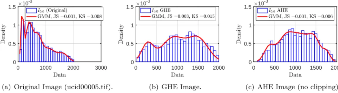
0 1000 2000 3000 0 0.5 1 1.5 10 -3

(a) Original Image (ucid00005.tif).

0 500 1000 1500 2000 0 0.5 1 1.5 10 -3 (b) GHE Image. 0 500 1000 1500 2000 0 0.5 1 1.5 10 -3

(c) AHE Image (no clipping).

Fig. 1: Characterization ofI0,0using GMM.

CLAHE suppresses enhancement of noise by limiting the highest value in image histogram known as Clip Limit (CL). The CLcan be defined as highest value allowed in a bin of histogram of an image tile. The density values which are greater than CL in a given image tile are redistributed. The CL and number of tiles (T) are two important parameters of CLAHE. In literature, it is stated that different probability den-sity functions (pdf)s (uniform, exponential, Rayleigh, etc.) for image histograms in HE for CLAHE are con-sidered based on applications. In addition to natural images [16] and [17], CLAHE also found its applica-tion in enhancement of medical images [13] and [14] and underwater images [15].

Since the use of CLAHE is spreading, the tools to detect the presence of AHE are also required. In this paper, the statistical characterization of block DC co-efficient of 2D 8×8 DCT coefficients is employed to classify original and HE images. HE images include GHE, AHE and CLAHE images. The block DC co-efficient of 2D 8×8 DCT coefficients is defined as an array made up of all DC coefficients from 8×8 block of DCT coefficients. In image forensics, the DCT coeffi-cient analysis is employed to detect tampering in JPEG compressed images [18] and [19]. Further, the statisti-cal characterization of DCT coefficients has been pop-ular for improvements in encoder/decoder for JPEG standard [20], [21], [22] and [23]. It may be noted that statistical characterization of block variance and AC DCT coefficients are recently employed to detect global contrast enhancement (or power-law transformation) [24].

In this work, a tool is developed using statistical pa-rameters obtained from fitting of block DC coefficient by Gaussian Mixture Model (GMM). The estimated parameters with other statistical parameters are ap-plied to train a 10-fold cross-validation Support Vec-tor Machine (SVM) [25]. The trained SVM classifier can be used to classify original and HE images. The proposed tool is independent of T and can detect the presence of HE for a large set of CL, all considered pdfs (uniform distribution, exponential distribution, Rayleigh distribution ) for image histograms and range

of gray levels ("full" and "original") used for equaliza-tion. By means of Receiver operating curves (ROC), the efficacy of the proposed tool for the classification of original and HE images is shown. Additionally, the per-formance of the tool in detection of CLAHE images for different CLs, Ts, image histogram equalization pdfs, and range of gray levels used in equalization is also discussed.

The paper is divided into four sections. Section 2. describes the statistical characterization of block DC DCT coefficients by GMM. The HE detection system and its detection algorithm with ROC curves of devel-oped classifiers are explained in Sec. 3. Section 4. concludes the paper.

2.

Statistical Characterization

of DC DCT Coefficients

2.1.

Gaussian Mixture Model

A GMM is a pdf which is the weighted sum of densities of Gaussian components defined as

p x|µi,X i , wi ! = K X i=1 wig x|µi,X i ! , (1)

wherexis D-dimensional continuous-valued data vec-tor, wi fori= 1,2,3, ..., K are the weights of mixture and K is the number of components. In Eq. (1), g is a D-dimensional Gaussian density which can be ex-pressed as g x|µi, X i ! = 1 2π(D/2) P_i (1/2)exp ( −1 2X 0 −1 X i X ) , (2)

where X = (x−µi), µi is mean vector, and P_i is

covariance matrix. It may be observed from Eq. (1), the sum of mixture weights (wi) for all components

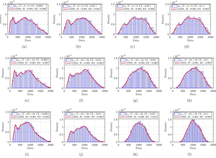
0 500 1000 1500 2000 0 0.5 1 1.5 10 -3 (a) 0 500 1000 1500 2000 0 0.5 1 1.5 10 -3 (b) 0 500 1000 1500 2000 0 0.5 1 1.5 10 -3 (c) 0 500 1000 1500 2000 0 0.5 1 1.5 10 -3 (d) 0 500 1000 1500 2000 0 0.5 1 1.5 10 -3 (e) 0 500 1000 1500 2000 0 0.5 1 1.5 10 -3 (f) 0 500 1000 1500 2000 0 0.5 1 1.5 10 -3 (g) 0 500 1000 1500 2000 0 0.5 1 1.5 10 -3 (h) 0 500 1000 1500 2000 0 0.5 1 1.5 10 -3 (i) 0 500 1000 1500 2000 0 0.5 1 1.5 2 10 -3 (j) 0 500 1000 1500 2000 0 0.5 1 1.5 2 10 -3 (k) 0 500 1000 1500 2000 0 0.5 1 1.5 2 10 -3 (l)

Fig. 2: Characterization ofI0,0 of CLAHE images using GMM with varyingCLandT (a), (e) and (i)CL= 0.005, (b), (f) and

(j)CL= 0.01, (c), (g) and (k)CL= 0.05, (d), (h) and (l)CL= 0.1. (a)-(d)T = 8×8, (e)-(h)T = 16×16, and (i)-(l)T

= 32×32, represents number of tiles used in CLAHE with uniform pdf and "full" range of gray levels.

is equals to 1. The parameters of GMM are: mean vector, covariance matrix, and mixture weights. These parameters can be collected to form a feature set (θ) given by, θ= ( wi, µi, X i ) , i= 1,2,3, ..., K. (3)

The model settings, like the number of components, type of covariance matrix, and sharing of parameters, depends on the size of available data for estimation of parameters and application. In our work, the diagonal covariance matrix for all components is used, and the parameters in Eq. (3) are estimated using Maximum Likelihood Estimation (MLE).

2.2.

Statistical Characterization

The DC coefficients of images are calculated in grayscale domain by employing type - II 8×8 block DCT of JPEG standard. The type-II DCT is defined

as I_u,vb =αu(u)αv(v) 7 X x=0 7 X y=0 ix,y cos _{π(2x+ 1)u} 16 cos _{π(2y+ 1)v} 16 , (4) wherex, yandu, vrepresent spatial and frequency do-main variables, respectively. The value of αu(u) and

αv(v) at u= 0, v = 0 is 1/√8. The DCT coefficient at u = 0, v = 0 is known as DC coefficient which is defined in type - II DCT as I₀b_,0= 1 8 7 X x=0 7 X y=0 ix,y, (5)

where I0b,0 is the DC coefficient of an image block, b

represents number of the block. It may be noted that

Ib

0,0 is eight times of the mean value of 8×8 block of

an image. The block DC coefficientI0,0can be defined

as

I0,0=

0 500 1000 1500 2000 0 0.5 1 1.5 10 -3 (a) 0 500 1000 1500 2000 0 0.5 1 1.5 2 10 -3 (b) 0 500 1000 1500 2000 0 0.5 1 1.5 10 -3 (c) 0 500 1000 1500 2000 0 0.5 1 1.5 2 10 -3 (d)

Fig. 3: Characterization ofI0,0of CLAHE images using GMM for (a)T = 8×8, exponential distribution (b)T = 8×8, Rayleigh

distribution, (c)T = 16×16, exponential distribution and (d)T = 16×16, Rayleigh distribution withCL= 0.01 and "full" range of gray levels.

0 500 1000 1500 2000 0 0.5 1 1.5 10 -3 (a) 0 500 1000 1500 2000 0 0.5 1 1.5 10 -3 (b) 0 500 1000 1500 2000 0 0.5 1 1.5 10 -3 (c) 0 500 1000 1500 2000 0 0.5 1 1.5 10 -3 (d)

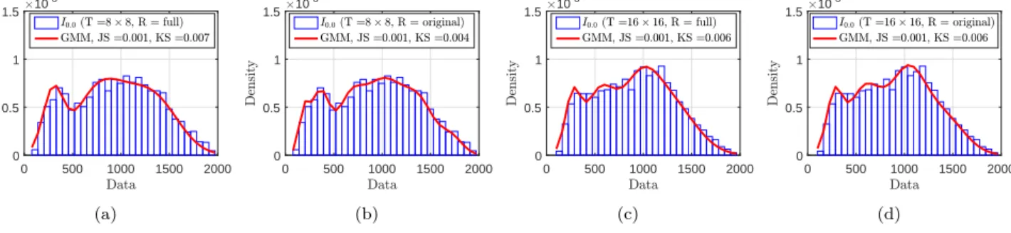
Fig. 4: Characterization ofI0,0of CLAHE images using GMM for (a)T = 8×8, "full" range (b)T = 8×8, "original" range, (c)

T = 16×16, "full" range and (d)T = 16×16, "original" range withCL= 0.01 and uniform distribution.

where B is number of 8×8 non-overlapping blocks in the input image. The histograms of I0,0 of original

image, histogram equalized image, and adaptive his-togram equalized image are characterized by GMM as shown in Fig. 1. The statistical characterization ofI0,0

of CLAHE images for different values of CLand T is shown in Fig. 2. The statistical characterization ofI0,0

of CLAHE images for different pdfs of histograms is shown in Fig. 3. The effect of the range of gray lev-els on characterization of I0,0 is shown in Fig. 4. In

the legend of Fig. 4, "full" represents the entire avail-able range of gray levels (i.e., 256 for 8-bit image), and "original" represents the range of gray levels in original image. The characterizations shown in Fig. 1, Fig. 2, Fig. 3 and Fig. 4 are obtained with optimum number of components found using Akaike Information Criterion (AIC) [26]. Further, to measure the efficacy of charac-terization, we have employed Jensen-Shannon (JS) di-vergence [27] and [28] and Kolmogorov-Smirnov (KS) statistic [29] and [28]. The values of JS and KS in dif-ferent cases of HE for a UCID [30] image are shown in legends of Fig. 1, Fig. 2, Fig. 3 and Fig. 4. A con-sistency in values of JS and KS concludes GMM as a good model of fit across original and different types of HE images.

2.3.

Parameter Analysis of CLAHE

To find the optimum number of components (K) for GMM, we have calculated the mean JS and KS values with varying K (1,3,5, . . . ,10) for all 1338 images of UCID database. It is worth mentioning that KS hy-pothesis test is performed withα= 0.01. The efficacy of GMM for characterization of I0,0 can be observed

from Tab. 1, Tab. 2, Tab. 3, Tab. 4 and Tab. 5.

Effect of CL: With an increase in the value ofCL

from 0.005 (large clipping) to 1 (no clipping), the shift in skewness from right to left of p(I0,0) is observed

(Fig. 2 and Fig. 3). Lower values ofCLrepresent low contrast, and higher values ofCLrepresent higher con-trast. Additionally, a decrease in kurtosis among dis-tributions can also be observed in Fig. 3. The effect of

CLin characterization ofp(I0,0) is tabulated in Tab. 1,

Tab. 2, Tab. 3 and Tab. 4 for different values ofT.

Effect of T: The effect of the number of tiles

T used in CLAHE is shown in Fig. 2. It may be observed from Fig. 2 that kurtosis of p(I0,0)

increases with increase of T. The Tab. 1, Tab. 2, Tab. 3 and Tab. 4 show variation of up to 2 % in mean JS and KS statistic values with varying T.

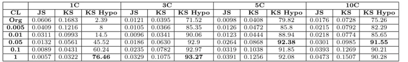
Tab. 1: Mean values of JS and KS and KS Hypothesis result forT = 8×8 (Org = Original).

1C 3C 5C 10C

CL JS KS KS Hypo JS KS KS Hypo JS KS KS Hypo JS KS KS Hypo

Org 0.0606 0.1683 2.39 0.0122 0.0395 71.52 0.0110 0.0441 80.12 0.0203 0.0813 75.86 0.005 0.0371 0.1185 7.55 0.0129 0.0439 85.13 0.0134 0.0497 86.62 0.0210 0.0816 76.83 0.01 0.0267 0.0944 14.72 0.0117 0.0412 89.24 0.0173 0.0603 89.61 0.0265 0.0919 87.44 0.05 0.0113 0.0528 40.96 0.0155 0.0528 94.25 0.0254 0.0829 92.83 0.0322 0.1046 91.33 0.1 0.0084 0.0438 52.84 0.0192 0.0644 93.2 0.0319 0.1028 92.53 0.0392 0.1258 90.66 1 0.0067 0.0378 63.45 0.0254 0.0834 93.2 0.039 0.1243 92.15 0.0448 0.1421 90.96

Tab. 2: Mean values of JS and KS and KS Hypothesis result forT = 16×16.

1C 3C 5C 10C

CL JS KS KS Hypo JS KS KS Hypo JS KS KS Hypo JS KS KS Hypo

Org 0.0606 0.1683 2.39 0.0121 0.0395 71.52 0.0098 0.0408 79.82 0.0176 0.0728 75.26 0.005 0.0409 0.1216 8 0.0105 0.0366 85.35 0.0126 0.0472 85.8 0.0215 0.0792 82.29 0.01 0.0311 0.0993 14.5 0.0096 0.0341 90.06 0.0123 0.0444 88.94 0.0218 0.0774 85.65 0.05 0.0132 0.0561 45.52 0.0186 0.0630 92.9 0.0264 0.0868 92.38 0.0301 0.0985 91.55 0.1 0.0089 0.0431 60.24 0.0235 0.0782 92.97 0.0319 0.1038 91.85 0.0393 0.1269 90.21 1 0.0057 0.0322 76.46 0.0329 0.1075 93.27 0.0391 0.1256 92.08 0.0473 0.1507 90.28

Tab. 3: Mean values of JS and KS and KS Hypothesis result forT = 32×32.

1C 3C 5C 10C

CL JS KS KS Hypo JS KS KS Hypo JS KS KS Hypo JS KS KS Hypo

Org 0.0606 0.1684 2.39 0.0121 0.0388 71.52 0.0098 0.0408 79.82 0.0229 0.0899 74.89 0.005 0.0482 0.1247 8.45 0.0148 0.0532 73.84 0.0192 0.0750 76.08 0.0321 0.1231 71.52 0.01 0.0413 0.1087 15.02 0.0135 0.0493 80.57 0.0224 0.0839 80.42 0.0324 0.1186 76.83 0.05 0.0201 0.0642 39.69 0.0202 0.0676 93.05 0.0280 0.0925 92.3 0.0368 0.1216 90.58 0.1 0.0130 0.0515 51.05 0.0271 0.0897 92.3 0.0321 0.1049 91.63 0.0421 0.1373 90.21 1 0.0063 0.0333 70.7 0.0418 0.1357 90.88 0.0474 0.1529 89.46 0.0522 0.1676 87.74

Tab. 4: Mean values of JS and KS and KS Hypothesis result forT = 64×64.

1C 3C 5C 10C

CL JS KS KS Hypo JS KS KS Hypo JS KS KS Hypo JS KS KS Hypo

Org 0.0606 0.1683 2.39 0.0125 0.0396 71.75 0.0107 0.0424 80.49 0.0237 0.0927 75.11 0.005 0.0438 0.1157 12.03 0.0164 0.0559 83.93 0.0234 0.0825 85.5 0.0339 0.1204 82.81 0.01 0.0438 0.1157 12.03 0.0164 0.0553 83.71 0.0244 0.0853 85.8 0.0313 0.1116 83.41 0.05 0.0332 0.0903 23.54 0.0199 0.0662 92.68 0.0286 0.0950 92.08 0.0401 0.1329 90.28 0.1 0.0252 0.0757 36.62 0.0255 0.0849 92.68 0.0338 0.1117 90.73 0.0411 0.1353 89.39 1 0.0129 0.0513 53.36 0.0307 0.1018 91.78 0.0392 0.1284 89.39 0.0444 0.1449 87

Tab. 5: Mean values of JS and KS and KS Hypothesis result for image HE pdfs (D1 = uniform distribution,D2= exponential

distribution andD3 = Rayleigh distribution) and range of gray levels (R1 = "full" andR2= "original").

1C 3C 5C 10C

JS KS KS Hypo JS KS KS Hypo JS KS KS Hypo JS KS KS Hypo

D1 _RR1 0.027 0.094 14.72 0.012 0.041 89.24 0.017 0.060 89.61 0.026 0.092 87.44 2 0.028 0.1 12.11 0.013 0.045 88.12 0.017 0.060 88.49 0.023 0.082 86.17 D2 R1 0.028 0.102 9.72 0.01 0.036 89.61 0.017 0.059 89.01 0.026 0.089 87.14 R2 0.029 0.108 8.37 0.012 0.0419 87.37 0.018 0.064 87.59 0.027 0.093 85.28 D1 _RR1 0.025 0.092 13.83 0.015 0.0514 92.08 0.023 0.075 92 0.029 0.095 89.91 2 0.025 0.094 13.38 0.014 0.0465 92.08 0.021 0.071 91.93 0.033 0.1081 89.24

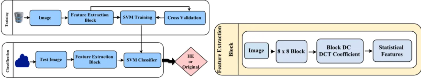
(a) For analysis and detection. (b) Feature extraction block.

Fig. 5: The system model.

Effect of image HE pdfs: As may be observed from Tab. 5, the maximum number of KS hypothesis tests is passed when the image histogram equalization pdf is a Rayleigh distribution.

Effect of range of gray levels in HE: The mean values of JS and KS statistic are the smallest (Tab. 5) when the chosen gray levels are in full range with uniform and exponential distribution. But in case of Rayleigh distribution, the chosen ranges of gray levels have no effect on the mean values of JS and KS statistics.

One can observe from Tab. 1, Tab. 2, Tab. 3, Tab. 4 and Tab. 5 that the optimum values of JS and KS statistic are obtained withK = 3 and 5. In our work, we have chosenK = 5 because the maximum number of KS hypothesis tests for original images is passed withK = 5. It is noteworthy that the mean values of JS and KS statistic are calculated after removing 5 % outliers from the original images database.

1. Ix,yt ← grayscale It

where, x = 0,1, ...7, y = 0,1, ...7, represents spatial domain.

2. Compute 8×8 2D block DCT, It

u,v ←DCT(Ix,yt )

where,u= 0,1, ...7, v= 0,1, ...7, represents frequency domain.

3. Compute the block DC Coefficient,It

0,0.

4. Estimate parameters by fitting block DC Coefficient,

It

0,0 to GMM (Eq. 2).

5. Create features set,F(Eq. 7).

6. ghe←SVMClassifier (F) here,he= 0 =⇒ original andhe= 1 =⇒ HE.

Fig. 6: Proposed HE detection algorithm.

3.

Histogram Equalization

Detection

3.1.

System Model for Analysis and

Detection

The system model used for analysis and detection is shown in Fig. 5. The GHE, AHE and CLAHE oper-ations are performed in spatial domain with 256 gray levels and saved in TIFF format. For CLAHE, theT

are 8×8,16×16,32×32 and 64×64 and the CL

are 0.005,0.01,0.03,0.05,0.07,0.09,0.1,0.3. Addition-ally, the CLAHE images are also generated with expo-nentially and Rayleigh distributed histograms for all considered Ts and CLs. For the range of gray levels in enhanced images, both "original" and "full" ranges are considered. For feature extraction (Fig. 5), the 2D 8×8 block DCT of the grayscale image is computed. The DC DCT coefficient of each block is collected to generate I0,0 (Eq. 6). It is observed (Fig. 1, Fig. 2,

Fig. 3, Fig. 4 and Fig. 5) that p(I0,0) is varying with

histogram equalization operations. Therefore, statis-tics ofI0,0can be used as features for classification.

Construction of the feature set involves the cal-culation of 10 − f old cross-validation accuracies of SVM classifiers for respective feature set. The accuracies corresponding to different feature sets for classification between original and GHE, orig-inal and AHE, origorig-inal and CLAHE (CL = 0.05,

D = D1, D2, D3, T = 8 × 8, R1) images are shown in Tab. 6. After experimentation, a 56-dimensional feature set F Eq. (7) is constructed and used for classification between original and all types

Tab. 6: 10−f oldcross-validation accuracies of SVM classifiers for different feature sets.

Features Number of features Org vs. GHE Org vs. AHE Org vs. CLAHE_(D1) Org vs. CLAHE_(D2) Org vs. CLAHE_(D3)

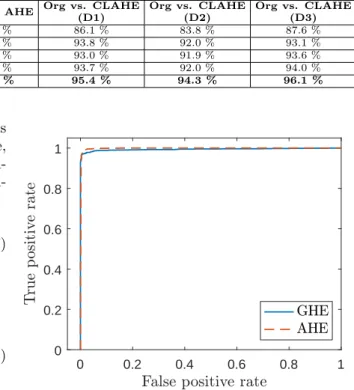
θ(Eq. 3) 15 86.7 % 88.7 % 86.1 % 83.8 % 87.6 %

S (Eq. 8) 11 98.8 % 97.0 % 93.8 % 92.0 % 93.1 %

p(I0,0) 30 95.7 % 97.4 % 93.0 % 91.9 % 93.6 %

θ+S 26 97.4 % 97.4 % 93.7 % 92.0 % 94.0 %

F (Eq. 7) 56 97.7 % 98.6 % 95.4 % 94.3 % 96.1 %

of histogram operations. The estimated parameters from GMM are combined with mean, median, mode, variance, skewness, kurtosis, minimum, maximum, en-tropy, energy of I0,0, number of peaks in I0,0 and

em-piricalp(I0,0). The feature setFis defined as

F={θ, p(I0,0), S}, (7)

where

S=nµ(I0,0), var(I0,0), Sk(I0,0), Ku(I0,0),

min(I0,0), max(I0,0), median(I0,0), mode(I0,0),

energy(I0,0), entropy(I0,0), peaks(I0,0)

o

. (8) The feature set Eq. (7) is applied to 10−f old cross-validation SVM with Radial Basis Function (RBF) ker-nel for training.

3.2.

Detection Algorithm and

Results

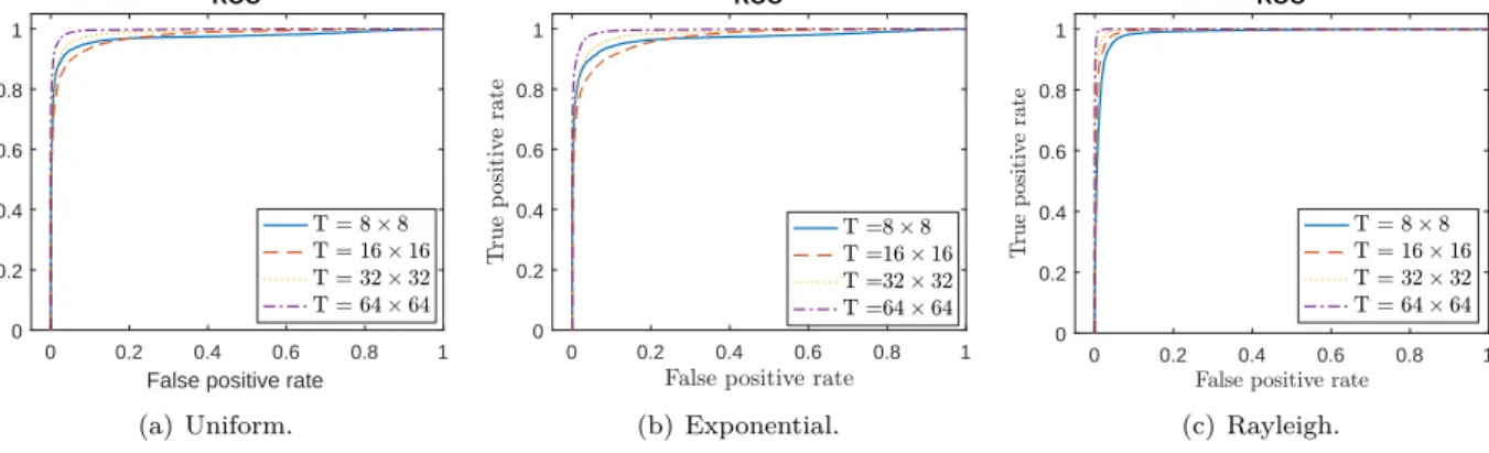
The proposed detection algorithm for classifying origi-nal and histogram equalized images is shown in Fig. 6. To test the efficacy of the proposed algorithm with im-portant parameters of GHE, AHE and CLAHE, we have created different simulation environments. The used database is UCID (TIFF format) with 1338 im-ages. The performance of proposed classifiers is shown in Fig. 7, Fig. 8, Fig. 9, Fig. 10 and Fig. 11 using 10−f old cross-validation ROC curves. The images are passed through GHE and AHE operation, and for preparation of feature matrix for each classification, the original images are mixed with corresponding HE images. The obtained ROC curves for classification be-tween original and each GHE and AHE are shown in Fig. 7. The simulation environments used for CLAHE are tabulated in Tab. 7.

The achieved TPR is > 95 % with FPR <5 % in most of the cases. TheCL= 0.005 represents less con-trast. Thus, the results atCL= 0.005 fall to 90 % with exponential distribution. In case of GHE and AHE, detection accuracy is more than 99 % with false alarm less than 1 %, which is comparable to existing methods [6] and [9], as shown in Tab. 8. The detection results for AHE and CLAHE are not reported in [6] and [9]. The proposed method is applicable with high efficacy for all types of histogram equalization operations.

0 0.2 0.4 0.6 0.8 1 0 0.2 0.4 0.6 0.8 1

Fig. 7: ROC curves for GHE and AHE classifier.

Tab. 7: Simulation environments of CLAHE. (D = distribu-tion,D1= uniform distribution,D2= exponential

dis-tribution and D3 = Rayleigh distribution) andR =

range of gray levels,R1 = "full" andR2 = "original",

"All" represents considered values ofT and CLas de-scribed in Sec. 3.1. Cases Parameters ROC varying constant T CL D R Case 1 T - All D1 R1 Fig. 8(a) D2 Fig. 8(b) D3 Fig. 8(c) Case 2 CL All -D1 R1 Fig. 9(a) D2 Fig. 9(b) D3 Fig. 9(c)

Case 3 D All All - R1 Fig. 10

Case 4 R All All All - Fig. 11

Tab. 8: Accuracy (TPR, FPR) of proposed method and exist-ing methods in HE based image Forensics.

Methods GHE AHE and CLAHE

Stamm[6] 100 %,3 % NA

Y uan[9] 100 %, 1 % NA

P roposed 99 %,1 % 99 %,1 % and 95 %,5 %

4.

Conclusion

The histogram equalization is a commonly used contrast enhancement technique. Its adaptive and contrast limited variant CLAHE is also spreading its footprint in application based image enhance-ments. We have developed a novel method to detect the presence of three commonly found

0 0.2 0.4 0.6 0.8 1 False positive rate

0 0.2 0.4 0.6 0.8 1

True positive rate

ROC (a) Uniform. 0 0.2 0.4 0.6 0.8 1 0 0.2 0.4 0.6 0.8 1 ROC (b) Exponential. 0 0.2 0.4 0.6 0.8 1 0 0.2 0.4 0.6 0.8 1 ROC (c) Rayleigh.

Fig. 8: ROC curves: HE detection for enhancement with varyingT for allCL.

0 0.2 0.4 0.6 0.8 1 0 0.2 0.4 0.6 0.8 1 ROC (a) Uniform. 0 0.2 0.4 0.6 0.8 1 0 0.2 0.4 0.6 0.8 1 ROC (b) Exponential. 0 0.2 0.4 0.6 0.8 1 0 0.2 0.4 0.6 0.8 1 ROC (c) Rayleigh.

Fig. 9: ROC curves: HE detection for enhancement with varyingCLfor allT.

0 0.2 0.4 0.6 0.8 1 0 0.2 0.4 0.6 0.8 1 ROC

Fig. 10: ROC curves for different pdfs used in CLAHE.

histogram equalization variants using statistical features. The proposed method employs statistical features of block DC coefficient to classify original and histogram equalized images. With few ex-ceptions, the proposed tool achieves higher accuracy

0 0.2 0.4 0.6 0.8 1 0 0.2 0.4 0.6 0.8 1 ROC

Fig. 11: ROC curves for different ranges used in CLAHE.

with all variants of histogram equalization. This tool does not involve image histograms based methods for detection of contrast enhancement and involves DC DCT coefficients, which is least affected by JPEG compression after enhancement.

References

[1] FARID, H. Image forgery detection.

IEEE Signal Processing Magazine. 2009, vol. 26, iss. 2, pp. 16–25. ISSN 1053-5888. DOI: 10.1109/MSP.2008.931079.

[2] REDI, J. A., W. TAKTAK and J. L. DUGE-LAY. Digital image forensics: a booklet for be-ginners.Multimedia Tools and Applications. 2011, vol. 51, iss. 1, pp. 133–162. ISSN 1573-7721. DOI: 10.1007/s11042-010-0620-1.

[3] QAZI, T., K. HAYAT, S. U. KHAN, S. A. MADANI, I. A. KHAN, J. KOODZIEJ, H. LI, W. LIN, K. C. YOW and C. Z. XU. Survey on blind image forgery detection.IET Image Process-ing. 2013, vol. 7, iss. 7, pp. 660–670. ISSN 1751-9659. DOI: 10.1049/iet-ipr.2012.0388.

[4] FARID, H. Blind inverse gamma correction.

IEEE Transaction on Image Processing. 2001, vol. 10, iss. 10, pp. 1428–1433. ISSN 1941-0042. DOI: 10.1109/83.951529.

[5] CAO, G., Y. ZHAO and R. NI. Forensic es-timation of gamma correction in digital im-ages. In: 17th IEEE International Conference on Image Processing (ICIP). Hong Kong: IEEE, 2010, pp. 2097–2100. ISBN 978-1-4244-7994-8. DOI: 10.1109/ICIP.2010.5652701.

[6] STAMM, M. C. and K. J. R. LIU. Foren-sic detection of image manipulation using sta-tistical intrinsic fingerprints. IEEE Transaction on Information Forensics and Security. 2010, vol. 5, iss. 3, pp. 492–506. ISSN 1556-6013. DOI: 10.1109/TIFS.2010.2053202.

[7] LIN, X., X. WEI and C. T. LI. Two Im-proved Forensic Methods of Detecting Contrast Enhancement in Digital Images. In:Media Water-marking, Security, and Forensics. San Francisco: SPIE, 2014, pp. 1–10. ISBN 978-0-819-49945-5. DOI: 10.1117/12.2038644.

[8] CAO, G., Y. ZHAO, R. NI and X. LI. Contrast enhancement-based forensics in digital images. IEEE Transaction on In-formation Forensics and Security. 2014, vol. 9, iss. 3, pp. 515–525. ISSN 1556-6021. DOI: 10.1109/TIFS.2014.2300937.

[9] YUAN, H. D. Identification of global histogram equalization by modeling gray-level cumulative distribution. In: IEEE China Summit & In-ternational Conference on Signal and Informa-tion Processing. Beijing: IEEE, 2013, pp. 645– 649. ISBN 978-1-4799-1043-4. DOI: 10.1109/Chi-naSIP.2013.6625421.

[10] CHEN, Z., Y. ZHAO and R. NI. Detec-tion for operaDetec-tion chain: Histogram equaliza-tion and dither-like operaequaliza-tion. KSII Transac-tions on Internet and Information Systems. 2015, vol. 9, iss. 9, pp. 3751–3770. ISSN 1976-7277. DOI: 10.3837/tiis.2015.09.026.

[11] PIZER, S. M., E. P. AMBURN, J. D. AUSTIN, R. CROMARTIE, A. GESELOWITZ, T. GREER, B. TER HAAR ROMENY, J. B. ZIMMERMAN and K. ZUIDERVELD. Adaptive histogram equalization and its variations. Com-puter vision, graphics, and image processing. 1987, vol. 39, iss. 3, pp. 355–368. ISSN 0734-189X. DOI: 10.1016/S0734-189X(87)80186-X

[12] ZUIDERVELD, K.Contrast limited adaptive his-togram equalization. San Diego: Academic Press Professional, Inc., 1994. ISBN 0-12-336155-9. [13] MAGUDEESWARAN, V. and J. F. SINGH.

Con-trast limited fuzzy adaptive histogram equaliza-tion for enhancement of brain images. Interna-tional Journal of Imaging Systems and Technol-ogy. 2017, vol. 27, iss. 1, pp. 98–103. ISSN 0899-9457. DOI: 10.1002/ima.22214.

[14] JUSTIN, J., J. SIVARAMAN, R. PERIYASAMY and V. R. SIMI. An objective method to identify optimum clip-limit and histogram specification of contrast limited adaptive histogram equalization for MR images. Biocybernetics and Biomedical Engineering. 2017, vol. 37, iss. 3, pp. 489–497. ISSN 0208-5216. DOI: 10.1016/j.bbe.2016.11.006. [15] OIAU, X., J. BAO, H. ZHANG, L. ZENG and D. LI. Underwater image quality enhance-ment of sea cucumbers based on improved histogram equalization and wavelet transform.

Information Processing in Agriculture. 2017, vol. 4, iss. 3, pp. 206–213. ISSN 2214-3173. DOI: 10.1016/j.inpa.2017.06.001.

[16] YADAV, G., S. MAHESHWARI and A. AGAR-WAL. Multi-domain image enhancement of foggy images using contrast limited adaptive histogram equalization method. In: Proceedings of the International Conference on Recent Cognizance in Wireless Communication and Image Process-ing. New Delhi: Springer, 2016, pp. 31–38. ISBN 978-81-322-2636-9. DOI: 10.1007/978-81-322-2638-3_4.

[17] JINTASUTTISAK, T. and S. INTAJAG. Color retinex image enhancement by Rayleigh contrast limited histogram equalization. In: International Conference on Control, Automation and Systems. Seoul: IEEE, 2014, pp. 692–697. ISBN 978-8-9932-1507-6. DOI: 10.1109/ICCAS.2014.6987868.

[18] YU, L., Q. HAN, X. NIU, S. M. YIU, J. FANG and Y. ZHANG. An improved pa-rameter estimation scheme for image modi-fication detection based on DCT coefficient analysis. Forensic Science International. 2016, vol. 259, iss. 1, pp. 200–209. ISSN 0379-0738. DOI: 10.1016/j.forsciint.2015.10.024.

[19] LIN, C. S. and J. J. TSAY. Passive forgery detection using discrete cosine transform coeffi-cient analysis in JPEG compressed images. Jour-nal of Electronic Imaging. 2016, vol. 25, iss. 3. ISSN 1017-9909. DOI: 10.1117/1.JEI.25.3.033010. [20] LAM, E. Y. and J. W. GOODMAN. A mathemat-ical analysis of the DCT coefficient distributions for images.IEEE Transaction on Image Process-ing. 2000, vol. 9, iss. 10, pp. 1661–1666. ISSN 1941-0042. DOI: 10.1109/83.869177.

[21] LAM, E. Y. Analysis of the DCT coefficient dis-tributions for document coding.IEEE Signal Pro-cessing Letters. 2004, vol. 11, iss. 2, pp. 97–100. ISSN 1070-9908. DOI: 10.1109/LSP.2003.821789. [22] NADARAJAH, S. and S. KOTZ. On the DCT

Coefficient Distributions. IEEE Signal Process-ing Letters. 2006, vol. 13, iss. 10, pp. 601–603. ISSN 1558-2361. DOI: 10.1109/LSP.2006.877141. [23] NADARAJAH, S. Gaussian DCT Coefficient

Models. Acta Applicandae Mathematicae. 2009, vol. 106, iss. 3, pp. 455–472. ISSN 1572-9036. DOI: 10.1007/s10440-008-9307-2.

[24] SINGH, N., A. GUPTA and R. C. JAIN. Global Contrast Enhancement Based Image Forensics Using Statistical Features. Advances in Electrical and Electronic Engineering. 2017, vol. 15, no. 3, pp. 509–516. ISSN 1804-3119. DOI: 10.15598/aeee.v15i3.2189.

[25] DUDA, R. O., P. E. HART and D. G. STORK.

Pattern Classification. 2nd ed. New York: Wiley, 2002. ISBN 978-0-471-05669-0.

[26] MCLACHLAN, G. and D. PEEL.Finite Mixture Models. New Jersey: Wiley, 2000. ISBN 978-0-471-00626-8.

[27] LIN J. Divergence measures based on the Shannon entropy. IEEE Transactions of Information The-ory. 1991, vol. 37, iss. 1, pp. 145–151. ISSN 0018-9448. DOI: 10.1109/18.61115.

[28] GUPTA A. and KARMESHU. Study of com-pound generalized Nakagami - generalized inverse Gaussian distribution and related densities: application to ultrasound imaging. Computa-tional Statistic. 2015, vol. 30, iss. 1, pp. 81—96. ISSN 0943-4062. DOI: 10.1007/s00180-014-0522-1.

[29] MASSEY, J. F. The Kolmogorov-Smirnov test for goodness of fit. Journal of the American statistical Association. 1951, vol. 46, iss. 253, pp. 68–78. ISSN 0162-1459. DOI: 10.1080/01621459.1951.10500769.

[30] SCHAEFER, G. and M. STICH. UCID: an un-compressed color image database.Storage and Re-trieval Methods and Applications for Multimedia. San Jose: SPIE, 2004, pp. 1–9. ISBN 978-0-8194-5275-7. DOI: 10.1117/12.525375.

About Authors

Neetu SINGH Ms. Neetu Singh received her B.Tech. (Electronics and Communication Engineer-ing) from IPEC, UP Technical University, Ghaziabad, and M.Tech. (Communication Systems and Signal Processing) from Jaypee Institute Of Information Technology (JIIT), Noida. She is pursuing her Ph.D. at JIIT, Noida. Presently working as an Assistant Professor in the Department Electronics and Commu-nication Engineering, JIIT, Noida.

Abhinav GUPTA Dr. Abhinav Gupta received his B.Tech. (Electrical Engg.) from I.E.T., M.J.P. Rohilkhand University, Bareilly, India and M.Tech. (Signal Processing) from I.I.T. Guwahati, India. He received his Ph.D. degree from School of Computer and Systems Sciences, Jawaharlal Nehru University, New Delhi in 2013. He was a senior chief engineer at Samsung Research and Development Institute, Delhi, India. Currently, he is an Associate Professor in the Department of Electronics and Communication Engineering, JIIT, Noida, India. His research interest include signal processing, statistical modelling and machine learning. He is an author and co-author of many scientific publications.

Roop Chand JAIN Prof. R. C. Jain has been working as the Head of Department and a Professor at the Department of Electronics and Communication Engineering, JIIT, Noida, India, since 2007. He received his BE in Electronics and Communication, ME in Microwaves and Radar from the University of Roorkee, Roorkee, MEngg (Electrical Engg.) and Ph.D. (Electrical Engg.) from the University of Alberta, Canada in 1988 under commonwealth Fellowship Programme of the Govt. of India. He worked in All India Radio (AIR) and Indian Airlines Corporation (IA) from 1971-1979 and 1979-1983, respectively. He joined BITS, Pilani, Rajasthan, as a Professor in Electrical and Electronics Group in 1989.