A Novel 2-Stage Combining Classifier Model with
Stacking and Genetic Algorithm based Feature Selection
Tien Thanh Nguyen1, Alan Wee-Chung Liew1, Xuan Cuong Pham2, Mai Phuong Nguyen3
1
School of Information Technology, Griffith University, Australia. 2
School of Information Technology, Hanoi University of Science and Technology, Vietnam 3
College of Business, Massey University, New Zealand
Email:[email protected]
Abstract. This paper introduces a novel 2-stage classification system with stacking and genetic algorithm (GA) based feature selection. Specifically, Lev-el1 data is first generated by stacking on the original data (called Level0 data) with base classifiers. Level1data is then classified by a second classifier (denot-ed by C) with feature selection using GA. The advantage of applying GA on Level1 data is that it has lower dimension and is more uniformity than Level0 data. We conduct experiments on both 18 UCI data files and CLEF2009 medi-cal image database to demonstrate superior performance of our model in com-parison with several popular combining algorithms.
Keywords: multiple classifier system, classifier fusion, combining classifiers, feature selection.
1
INTRODUCTION
Combining classifiers to improve classification performance has been shown to be an effective strategy [1-4]. In general, the more the differences in the training sets, base classifiers and feature sets, the better the combining output will be since they tend to capture different aspects of the classification task. Duin [1] summarized six combining strategies for multiple classifier systems: (a) different initializations, (b) different parameter choices, (c) different architectures, (d) different classifiers, (e) different training sets, and (f) different feature sets. In a two stage classification mod-el, the base classifiers are normally chosen to be significantly difference to each other. To train the base classifiers, Ting [5] developed the Stacking Algorithm where the training set is divided into several equal disjoint parts and each part plays as the test set once while the others play as the training set. The output of Stacking-based algo-rithms is a set of fuzzy label [2], which gives the posterior probability that each ob-servation belongs to an individual class according to each classifier. The set of poste-rior probability of all observation is called Level1 data. Let N as the number of ob-servations,K as the number of base classifiers and M as the number of classes
{ }
Wj2014 International Conference on Intelligent Computing, ICIC2014, Taiyuan, China, (LNCS, Vol. 8589, pp 33-43)
. For each observationXi, Pk(W |j Xi) is the probability that Xi belongs to class Wj
given by the th
k classifier. The Level1 data of all observations, a N×MK-posterior probability matrix
{
Pk(W |j Xi)}
j=1,M k=1,K i=1,N,is defined by:1 1 1 1 1 1 1 1 1 1 2 1 2 1 2 2 1 1 1 1 (W | )... (W | ) ... (W | )... (W | ) (W | )... (W | ) ... (W | )... (W | ) (W | )... (W | ) ... (W | )... (W | M K K M M K K M N M N K N K M P X P X P X P X P X P X P X P X P X P X P X P ) N X (1)
The Level1 data of an observationX is defined by:
1 1 1 1 (W | ) (W | ) 1( ) : (W | ) (W | ) M K K M P X P X Level X P X P X = (2)
Based on stacking, several well-known combining classifiers algorithms were introduced. Kuncheva [3] defined Decision Profile (denoted by DP X( )) of an observation X as equal to Level1(X) (eqn. 2) and Decision Template of ith class (denoted by DTi) as average of Decision Profile of observations in training set where their labels are Wi. Based on measurement between DTi(i=1,M ) and DP X( ), class label of X is predicted. Merz [11] proposed an algorithm called SCANN which first uses stacking result and the true label of learning set to build indicator matrix and applied Correspondence Analysis (CA) to that matrix to understand the relationship between observation and its class label. Then, K Nearest Neighbor is used to classify unlabeled observation on the Level1 data based on output of CA.
Kittler [18] introduced fixed rules to combine outputs from classifiers. The difference between fixed rules and trainable combining algorithms is that fixed rule is pre-chosen and does not involve training on Level1 data.. Six fixed combing rules evaluated in this paper are Sum, Product, Max, Min, Median and Majority Vote.
Two interesting questions related to multi classifier system are whether there exist a subset of base classifiers and a subset of features that could achieve better classification results than the original sets? The first question is classifier selection problem. It means that in some situations, system with the elimination of some base classifiers may perform better than system with all base classifiers. The second ques-tion, which is the main subject of this paper, is feature selection. The purpose of this task is to reduce the number of features from feature set while still maintaining ac-ceptable accuracy. In fact, some attributes of an object may have low discriminative power because of their nature and measurement bias. As a result, subset formed by removing these attributes may be more discriminative than its superset.
3
2
RECENT WORK
2.1 2-Stage model
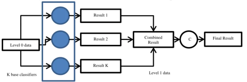
The idea of 2-stage model was published in [6] where K different feature vec-tors extracted from an object is used by K base classifiers respectively. However, extracting K feature vectors from an object is not always feasible so here we propose applying Stacking Algorithm to the 2-stage model as illustrated in Fig. 1. In the first stage, the dataset is classified by K base classifiers by Stacking and their output is Level1 data (eqn. 1). Next, the Level1 data is classified by a new classifier (denoted by C in Fig.1). Level1 data can be viewed as “scaled results” given by K base classi-fiers (Level1 data is real value scaled in [0, 1]).
Our proposed model is very flexible in that the base classifiers can be chosen as different as possible (Strategy d) [1] while C is another arbitrary classifier. Here, the K base classifiers play the role of generating Level1 data from Level0 data by stacking, and then this new data is classified by C. Our aim is to gain lower error rate in comparison to when C is applied directly to Level0 data (classification directly by C), best result from all base classifiers, as well as popular combining classifier algo-rithms namely fixed rules, SCANN [11] and Decision Template [2].
Fig. 1. Proposed 2-Stage model based on Stacking Algorithm
2.2 GA in multi classifier system
Feature selection is an important technique in pattern recognition, data anal-ysis and data mining [7]. Generally speaking, methods that transform features to a new domain with a reduction in the dimension of feature can be treated as feature selection. Therefore, strategy to solve this problem is very diverse, for instance, linear transformations, search techniques and Genetic Algorithm (GA). Here, we review literatures about GA for multi classifier system.
Kuncheva [4] introduced join and disjoin mechanism for GA approach. First-ly, chromosome was encoded by
{
0,1,...,K}
where k (1≤ ≤k K) means that feature associated with this point is only used by thk classifier and 0 is otherwise. In the sec-ond version, classifier encoding was added in the same chromosome with feature encoding, in which Venn diagram and integer values were used for feature and classi-fier encoding, respectively. In Kuncheva’s experiment, the first version was not good while the second version is hard to implement since Venn diagram becomes more
Level 0 data Result 1 Result 2 Result K Combined Result Final Result Level 1 data K base classifiers C
complicated with many classifiers. Nanni [9] employed GA to improve SCANN algo-rithm [11] by building representations where each includes encoding of M classes. Gabrys [8] tried to put classifier, feature and rule encoding in a single chromosome as a 3-dimensional cube. However, the above 2 approaches are hard to implement be-cause of complicated crossover stage.
In our experiments, error rates of classification task on Level1 data of several data sources are not significantly improved compared with that of classification di-rectly by C. It motivated us to apply GA on Level1data in order to achieve lower error rate. In the next section, we propose a novel chromosome encoding on Level1 data. After that, empirical evaluations are conducted on 18 UCI data files and CLEF 2009 medical image database to compare its performance with several existing algorithms. Finally, we conclude with some discussion about future developments.
3
2-STAGE GA ON LEVEL1 DATA
As mention above, Level1 data usually has fewer dimension than Level0 da-ta, for example, binary classification by 3 base classifiers only generates Level1 data with 6 dimensions. So if GA is applied to Level1 data, it saves computation cost by reducing the number of initial chromosomes in population while still has good oppor-tunity to achieve global optimum. Besides, Level1 data can be viewed as transfor-mation from feature domain to posterior domain where data is reshaped by posterior probability. Observations that belong to the same class have greater chance to locate nearby in the new domain. Therefore, it is expected that Level1 data will have more discriminative power than the original data.
As mentioned above, each base classifier outputs the predictions as posterior probability values that an observation is belonged to predefined classes. Outcome of combining classifiers algorithm may be degraded by unreliable predictions from base classifiers. The idea of feature selection on Level1 data is to select reliable predictions of a base classifier for combining algorithms and discard unreliable predictions. As a result, the discriminant ability of new Level1 data is more power than the original Level1 data.
To apply GA on Level1 data, we propose the following chromosome struc-ture. Each chromosome includes M×K genes due to the number of features of Lev-el1 data. We use two elements {0,1} to encode for each gene in a chromosome in which: 1 if feature is selected ( ) 0 otherwise th i Gene i = (3)
At crossover stage, we employ single splitter since the same single random point is selected on all pairs of parents. Each parent exchanges its head with the other while keeps its tail. After this stage, two new offspring chromosomes are generated. Next, based on mutation probability, we select random genes on two offspring chro-mosomes and change its values by 0→1 or 1→0. This mutation helps GA reach not only local extreme values but also global one. Here we select the accuracy of classifi-er C as fitness value of GA. Our GA approach is detailed below:
5
Algorithm 1: GA on Level1 data Training procedure:
Input: Level0 data, K base classifiers, classifier C, TMax: number of interaction, PMul: mutation probability, L: population size
Output: optimal subset of Level1 feature and classification model. Step1: Initialize a population with L random chromosomes
Step2: Compute fitness function of each initialized chromosome by cross validation method on Leve1l data of training set and then classify by C.
Step3: Loop to select N best chromosomes. Do
• Withdraw with replacement L/2 pairs from population, conduct
crossover and mutation (based on PMul) to generate new L chro-mosomes.
• Add new L chromosomes to population.
• Compute fitness value of new chromosomes
• Select new population with L best fitness value chromosomes.
While (converge = true)
Step4: Select optimal chromosome from final population.
Step5: Build classification model based on encoding of best chromo-some.
Test process: Input: unlabeled observation XTest. Output: predicted label of XTest.
Step1: Compute Level1 data of XTest
Step2: Select features from Level1 of XTest based on optimal chro-mosome encoding.
Step3: Classify selected features by C.
4
EXPERIMENTAL RESULTS
We conducted experiments on several types of data namely UCI data files [13] and CLEF 2009 medical image database. Since only a single dataset was availa-ble for both training and testing, 10-fold cross validation was performed. The proce-dure was run 10 times so a total of 100 test results were obtained. In our assessment, we compared the error rates of 11 methods: six fixed rules (Sum, Product, Max, Min, Median and Majority Vote), best result from base classifiers, classification directly by C, 2-stage model, two well-known combining algorithms (Decision Template and SCANN) and our 2-stage model with Level1 feature selection by GA (2-stage GAFS). To initialize parameters of GA, we set mutation probability PMul = 0.015, population size L = 20. Three base classifiers namely Linear Discriminant Analysis (LDA), Na-ïve Bayes and K Nearest Neighbor (with K set to 5, denoted as 5-NN)are selected. The second classifier C isa Decision Tree. Finally, paired t-test was used (level of significance set to 0.05) on the results of our model and a benchmark algorithm for statistical significance.
4.1 UCI Data files
We chose 18 data files with 2 classes (Bupa, Artificial, Sonar, etc…) to 6 classes (Dermatology). The number of attributes also changes in a wide range from only 3 (Haberman) to 60 (Sonar). The number of observations in each file also varies
considerably, from small files like Fertility to quite big files such as Skin&NonSkin (Table1). Our purpose is to conduct an objective experiment to evaluate the advantage of our approach for a diversity of data sources. At the preprocessing step, we remove missing observations. Experimental results on all 18 files are summarized in Table 2, 3, 4 and 5.
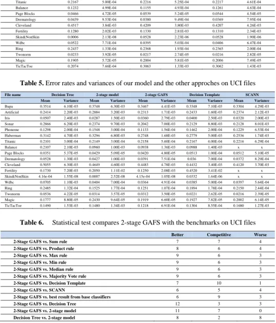
First, it is interesting to note that classification result from the 2-stage model is not significant better than classification directly by Decision Tree on Level0 data. There are 8 cases where direct classification by Decision Tree is better than the 2-stage model and 8 cases where performance is worse. The proposed 2-2-stage GAFS model, on the other hand, is significantly better than both Decision Tree and the 2-stage model. Our model obtained 12 wins and only 3 losses compared with the former and 11 wins and 0 loss compared with the latter.
Next, we compare the 2-Stage GAFS approach to the best result from three base classifiers. The 2-stage GAFS approach has superior performance in 6 files, namely Artificial (0.2313 vs. 0.2496), Balance (0.0938 vs. 0.1442), Fertility (0.125 vs. 0.155), Skin&NonSkin (4.15e-04 vs. 5e-04), Ring (0.1251 vs. 0.2374) and TicTacToe (0.1218 vs. 0.1557), while it has inferior performance in 3 files: Iris (0.036 vs. 0.02), Haberman (0.2748 vs. 0.2596) and Twonorm (0.0312 vs. 0.0217).
Then, two well-known combining classifiers algorithms, namely SCANN and Decision Template, are compared with our 2-Stage GAFS model. Unfortunately, SCANN cannot be performed on Balance, Skin&NonSkin and Fertility files because the indicator matrix has columns with all 0 posterior probability values from the K base classifiers. As a result, its column mass will be singular and the standardized residuals is not available. These files are not included in the comparison with our model. SCANN outperforms 2-Stage GAFS model on 4 files and underperforms on 6 files. Decision Template, in turn, obtains only 1 win and 7 losses among the 18 files. Significant results are Phoneme (0.1133, 0.1462 and 0.1229), Ring (0.1251, 0.1894 and 0.2150) and TicTacToe (0.1218, 0.1304 and 0.1680) for 2-Stage GAFS, Decision Template and SCANN, respectively. Besides, comparing with 6 fixed combining rules, our model achieves 7 wins and 4 losses (Sum rules), 8 wins and 4 losses (Prod-uct Rules) and 9 wins and 3 losses (Max, Min, Median and Majority Vote rule).
Finally, the dimensions of Level0 data, Level1 data and data of 2-Stage GAFS model are compared. From Fig. 2 we can see that GA helps reduce the number of features significantly while error rate is maintained at acceptable value (Table 4). There are only 4 files, Iris, Balance, Titanic and Page Blocks, where GAFS approach gives higher dimension than that of Level0 data; i.e. 1, 3, 2 and 1 higher, respectively. However, in the others files, the proposed GA outperforms Level0 data, especially on 4 files: Sonar (1 vs. 60), Artificial (1 vs. 10), Ring (1 vs. 20) and Twonorrn (2 vs. 20).
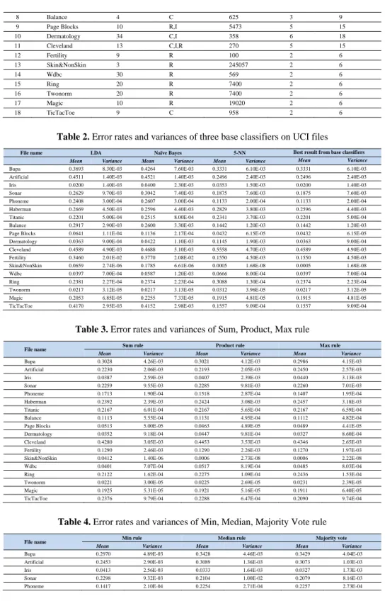
Table 1. UCI data files used in our experiment
File name # of attributes Attribute Type # of observations # of classes # of attribute on Level1 (3 classifiers) 1 Bupa 6 C,I,R 345 2 6 2 Artificial 10 R 700 2 6 3 Iris 4 R 150 3 9 4 Sonar 60 R 208 2 6 5 Phoneme 5 R 540 2 6 6 Haberman 3 I 306 2 6 7 Titanic 3 R,I 2201 2 6
7
8 Balance 4 C 625 3 9
9 Page Blocks 10 R,I 5473 5 15
10 Dermatology 34 C,I 358 6 18 11 Cleveland 13 C,I,R 270 5 15 12 Fertility 9 R 100 2 6 13 Skin&NonSkin 3 R 245057 2 6 14 Wdbc 30 R 569 2 6 15 Ring 20 R 7400 2 6 16 Twonorm 20 R 7400 2 6 17 Magic 10 R 19020 2 6 18 TicTacToe 9 C 958 2 6
Table 2. Error rates and variances of three base classifiers on UCI files
File name LDA Naïve Bayes 5-NN Best result from base classifiers
Mean Variance Mean Variance Mean Variance Mean Variance Bupa 0.3693 8.30E-03 0.4264 7.60E-03 0.3331 6.10E-03 0.3331 6.10E-03 Artificial 0.4511 1.40E-03 0.4521 1.40E-03 0.2496 2.40E-03 0.2496 2.40E-03 Iris 0.0200 1.40E-03 0.0400 2.30E-03 0.0353 1.50E-03 0.0200 1.40E-03 Sonar 0.2629 9.70E-03 0.3042 7.40E-03 0.1875 7.60E-03 0.1875 7.60E-03 Phoneme 0.2408 3.00E-04 0.2607 3.00E-04 0.1133 2.00E-04 0.1133 2.00E-04 Haberman 0.2669 4.50E-03 0.2596 4.40E-03 0.2829 3.80E-03 0.2596 4.40E-03 Titanic 0.2201 5.00E-04 0.2515 8.00E-04 0.2341 3.70E-03 0.2201 5.00E-04 Balance 0.2917 2.90E-03 0.2600 3.30E-03 0.1442 1.20E-03 0.1442 1.20E-03 Page Blocks 0.0641 1.11E-04 0.1136 2.17E-04 0.0432 6.15E-05 0.0432 6.15E-05 Dermatology 0.0363 9.00E-04 0.0422 1.10E-03 0.1145 1.90E-03 0.0363 9.00E-04 Cleveland 0.4589 4.90E-03 0.4688 5.10E-03 0.5558 4.70E-03 0.4589 4.90E-03 Fertility 0.3460 2.01E-02 0.3770 2.08E-02 0.1550 4.50E-03 0.1550 4.50E-03 Skin&NonSkin 0.0659 2.74E-06 0.1785 6.61E-06 0.0005 1.68E-08 0.0005 1.68E-08 Wdbc 0.0397 7.00E-04 0.0587 1.20E-03 0.0666 8.00E-04 0.0397 7.00E-04 Ring 0.2381 2.27E-04 0.2374 2.23E-04 0.3088 1.30E-04 0.2374 2.23E-04 Twonorm 0.0217 3.12E-05 0.0217 3.13E-05 0.0312 3.96E-05 0.0217 3.12E-05 Magic 0.2053 6.85E-05 0.2255 7.33E-05 0.1915 4.81E-05 0.1915 4.81E-05 TicTacToe 0.4170 2.95E-03 0.4152 2.98E-03 0.1557 9.09E-04 0.1557 9.09E-04
Table 3. Error rates and variances of Sum, Product, Max rule
File name Sum rule Product rule Max rule
Mean Variance Mean Variance Mean Variance Bupa 0.3028 4.26E-03 0.3021 4.12E-03 0.2986 4.15E-03 Artificial 0.2230 2.06E-03 0.2193 2.05E-03 0.2450 2.57E-03 Iris 0.0387 2.59E-03 0.0407 2.39E-03 0.0440 3.13E-03 Sonar 0.2259 9.55E-03 0.2285 9.81E-03 0.2260 7.01E-03 Phoneme 0.1713 1.90E-04 0.1518 2.87E-04 0.1407 1.95E-04 Haberman 0.2392 2.39E-03 0.2424 3.08E-03 0.2457 3.18E-03 Titanic 0.2167 6.01E-04 0.2167 5.65E-04 0.2167 6.59E-04 Balance 0.1113 5.55E-04 0.1131 4.95E-04 0.1112 4.82E-04 Page Blocks 0.0513 5.00E-05 0.0463 4.89E-05 0.0489 4.41E-05 Dermatology 0.0352 9.18E-04 0.0447 9.81E-04 0.0327 8.60E-04 Cleveland 0.4280 3.05E-03 0.4453 3.53E-03 0.4346 2.65E-03 Fertility 0.1290 2.46E-03 0.1290 2.26E-03 0.1270 1.97E-03 Skin&NonSkin 0.0412 1.40E-06 0.0006 2.73E-08 0.0006 2.22E-08 Wdbc 0.0401 7.07E-04 0.0517 8.19E-04 0.0485 8.03E-04 Ring 0.2122 1.62E-04 0.2275 1.09E-04 0.2436 1.53E-04 Twonorm 0.0221 3.00E-05 0.0225 2.69E-05 0.0231 2.39E-05 Magic 0.1925 5.31E-05 0.1921 5.16E-05 0.1911 6.40E-05 TicTacToe 0.2376 9.79E-04 0.2288 6.47E-04 0.2090 9.74E-04
Table 4. Error rates and variances of Min, Median, Majority Vote rule
File name Min rule Median rule Majority vote
Mean Variance Mean Variance Mean Variance Bupa 0.2970 4.89E-03 0.3428 4.46E-03 0.3429 4.04E-03 Artificial 0.2453 2.90E-03 0.3089 1.36E-03 0.3073 1.03E-03 Iris 0.0413 2.56E-03 0.0333 1.64E-03 0.0327 1.73E-03 Sonar 0.2298 9.32E-03 0.2104 1.00E-02 0.2079 8.16E-03 Phoneme 0.1417 2.10E-04 0.2254 2.71E-04 0.2257 2.73E-04
Haberman 0.2461 2.47E-03 0.2524 1.67E-03 0.2504 1.76E-03 Titanic 0.2167 5.00E-04 0.2216 5.25E-04 0.2217 4.61E-04 Balance 0.1232 4.99E-04 0.1155 4.93E-04 0.1261 4.63E-04 Page Blocks 0.0466 4.72E-05 0.0539 5.24E-05 0.0544 4.54E-05 Dermatology 0.0439 9.53E-04 0.0380 9.49E-04 0.0369 7.95E-04 Cleveland 0.4517 3.84E-03 0.4209 3.80E-03 0.4207 4.26E-03 Fertility 0.1280 2.02E-03 0.1330 2.81E-03 0.1310 2.34E-03 Skin&NonSkin 0.0006 2.13E-08 0.0528 2.23E-06 0.0528 1.90E-06 Wdbc 0.0522 7.71E-04 0.0395 5.03E-04 0.0406 6.47E-04 Ring 0.2437 1.33E-04 0.2368 1.93E-04 0.2365 2.00E-04 Twonorm 0.0233 3.92E-05 0.0217 2.74E-05 0.0216 2.82E-05 Magic 0.1905 5.72E-05 0.2004 5.81E-05 0.2006 7.49E-05 TicTacToe 0.2074 7.66E-04 0.3063 1.33E-03 0.3062 1.43E-03
Table 5. Error rates and variances of our model and the other approches on UCI files
File name Decision Tree 2-stage model 2-stage GAFS Decision Template SCANN
Mean Variance Mean Variance Mean Variance Mean Variance Mean Variance Bupa 0.3514 6.10E-03 0.3748 6.30E-03 0.3467 4.41E-03 0.3348 7.10E-03 0.3304 4.29E-03 Artificial 0.2414 2.20E-03 0.2884 3.20E-03 0.2313 1.71E-03 0.2433 1.60E-03 0.2374 2.12E-03 Iris 0.0507 2.40E-03 0.0287 1.50E-03 0.0360 2.79E-03 0.0400 2.50E-03 0.0320 2.00E-03 Sonar 0.2866 6.20E-03 0.2374 9.70E-03 0.2042 7.00E-03 0.2129 8.80E-03 0.2128 8.01E-03 Phoneme 0.1298 2.00E-04 0.1548 3.00E-04 0.1133 1.56E-04 0.1462 2.00E-04 0.1229 6.53E-04 Haberman 0.3142 4.70E-03 0.3296 6.80E-03 0.2748 1.68E-03 0.2779 5.00E-03 0.2536 1.74E-03 Titanic 0.2101 3.00E-04 0.2149 3.00E-04 0.2158 5.60E-04 0.2167 6.00E-04 0.2216 6.29E-04 Balance 0.2107 2.10E-03 0.0960 1.00E-03 0.0938 1.36E-03 0.0988 1.40E-03 x x Page Blocks 0.0351 5.37E-05 0.0429 5.09E-05 0.0420 4.80E-05 0.0513 1.00E-04 0.0512 5.10E-05 Dermatology 0.0528 1.30E-03 0.0427 1.00E-03 0.0391 7.51E-04 0.036 7.00E-04 0.0372 8.29E-04 Cleveland 0.5055 6.30E-03 0.4649 4.60E-03 0.4483 4.78E-03 0.4432 3.40E-03 0.4120 3.70E-03 Fertility 0.1730 7.20E-03 0.2050 1.11E-02 0.1250 2.08E-03 0.4520 3.41E-02 x x Skin&NonSkin 4.16e-04 1.55E-08 0.0007 2.52E-08 4.15e-04 1.05E-08 0.0332 1.64E-06 x x Wdbc 0.0705 1.10E-03 0.0404 7.00E-04 0.0364 4.91E-04 0.0385 5.00E-04 0.0397 5.64E-04 Ring 0.2485 1.32E-04 0.1525 1.77E-04 0.1251 1.07E-04 0.1894 1.78E-04 0.2150 2.44E-04 Twonorm 0.0536 4.22E-05 0.0314 3.57E-05 0.0312 3.50E-05 0.0221 2.62E-05 0.0216 2.39E-05 Magic 0.1777 8.80E-05 0.2430 9.64E-05 0.1919 6.60E-05 0.1927 7.82E-05 0.2002 6.14E-05 TicTacToe 0.1490 1.53E-03 0.1480 1.34E-03 0.1218 6.91E-04 0.1304 8.55E-04 0.1680 1.27E-03
Table 6. Statistical test compares 2-stage GAFS with the benchmarks on UCI files Better Competitive Worse
2-Stage GAFS vs. Sum rule 7 7 4
2-Stage GAFS vs. Product rule 8 6 4
2-Stage GAFS vs. Max rule 9 6 3
2-Stage GAFS vs. Min rule 9 6 3
2-Stage GAFS vs. Median rule 9 6 3
2-Stage GAFS vs. Majority Vote rule 9 6 3 2-Stage GAFS vs. Decision Template 7 10 1
2-Stage GAFS vs. SCANN 6 5 4
2-Stage GAFS vs. best result from base classifiers 6 9 3
2-Stage GAFS vs. Decision Tree 12 3 3
2-Stage GAFS vs. 2-stage model 11 7 0
9
Fig. 2. Comparing dimensions of data on UCI files** change name of 2 stage ga level 1
4.2 CLEF2009
The CLEF2009 medical image dataset collected by Archen University in-cludes 15363 medicalimages which are allocated to 193 hierarchical categories. In-formation about images in this dataset and their class is showed in Table 7. The imag-es are first histogram equalized and then the feature vector of image is extracted using Histogram of Local Binary Pattern (HLBP) [12]. The base classifiers we used are LDA, Quadratic Discriminant Analysis (QDA) and Naïve Bayes, and C is 5-NN. By changing base classifiers and C, we want to illustrate the flexible characteristic of our model. Experimental results are illustrated in Table 8.
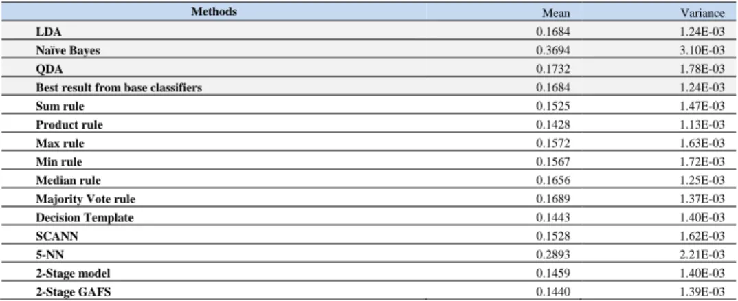
Again, the benefits of our 2-stage GAFS approach are obvious. It helps re-duce both the dimensions of feature on Level1 data and the error rates on the 10-class dataset. Our 2-Stage GAFS outperforms (paired t-test at p = 0.05) best result from base classifiers, 5 fixed rules (Sum, Max, Min, Median and Majority Vote) and 5-NN and is competitive with 2-stage model, Product rule, Decision Template and SCANN. Besides, the dimension of data is reduced from 32 to 30 and then 25 in the case of Level0 data, Level1data and 2-Stage GAFS, respectively.
Table 7. Information of CLEF2009 medical images
Image
Description Abdomen Cervical Chest Facial cranium Left Elbow
Number of observation 80 81 80 80 69
Image
Description Left Shoulder Left Breast Finger Left Ankle Joint Left Carpal Joint
6 10 4 60 5 3 3 4 10 34 13 9 3 30 20 20 10 9 6 6 9 6 6 6 6 9 15 18 15 6 6 6 6 6 6 6 2 1 5 1 2 1 5 7 11 17 5 2 1 6 1 2 1 2 0 10 20 30 40 50 60 70
Number of observation 80 80 66 80 80
Table 8. Error rates and variances of base classifiers and 6 approaches on CLEF2009
Methods Mean Variance
LDA 0.1684 1.24E-03
Naïve Bayes 0.3694 3.10E-03
QDA 0.1732 1.78E-03
Best result from base classifiers 0.1684 1.24E-03
Sum rule 0.1525 1.47E-03
Product rule 0.1428 1.13E-03
Max rule 0.1572 1.63E-03
Min rule 0.1567 1.72E-03
Median rule 0.1656 1.25E-03
Majority Vote rule 0.1689 1.37E-03
Decision Template 0.1443 1.40E-03
SCANN 0.1528 1.62E-03
5-NN 0.2893 2.21E-03
2-Stage model 0.1459 1.40E-03
2-Stage GAFS 0.1440 1.39E-03
5
CONCLUSION AND FUTURE WORK
In this paper, we have introduced a novel multi classifier system based on Stacking Algorithm and GA feature selection in which GA feature selection is applied on Level1 data. Our aim is not only to build an effective classification model but also to find a subset of Level1 data which have better discriminative power than its super-set. Extensive experiments on 18 UCI data files and CLEF2009 have demonstrated the benefits of our 2-Stage GA feature selection approach on Level1 data.
In the near future, we plan to improve our model by combining it with GA approach on Level0 data to solve both the feature and classifier selection problems in multi classifier systems. It is expected to result in significantly better combining clas-sifiers model.
REFERENCES
[1] Robert P. W. Duin, The Combining Classifier: To Train or Not to Train? Proceed-ings. 16th International Conference on Pattern Recognition, Vol 2, pp.765-770, 2002. [2] L. I. Kuncheva, James C. Bezdek and Robert P. W. Duin, Decision Templates for Multi Classifier Fusion: An Experimental Comparison, Pattern Recognition, Vol. 34, No. 2, pp.299-314, 2001.
[3] L. I. Kuncheva, A theoretical Study on Six Classifier Fusion Strategies, IEEE Transactions on Pattern Analysis and Machine Intelligence, Vol. 24, No. 2, February 2002.
[4] L. I. Kuncheva and Lakhmi C. Jain, Designing Classifier Fusion Systems by Ge-netic Algorithms, IEEE Transactions on Evolution Computation. Vol. 4, No. 4, Sep-tember 2000.
[5] Kai Ming Ting, Ian H. Witten, Issues in Stacked Generation, Journal of Artificial In Intelligence Research, Vol. 10, pp.271-289, 1999.
11
[6] L. Lepisto, I. Kunttu, J. Autio and A. Visa, Classification of Non-Homogeneous Texture Images by Combining Classifier, Proceedings International Conference on Image Processing, Vol. 1, pp.981-984, 2003.
[7] Micheal L.Raymer, William F.Punch, Erik D.Goodman, Leslie A.Kuhn and Anil K.Jain, Dimensionality Reduction using Genetic Algorithms, IEEE Transactions on Evolutionary Computation, Vol. 4, No. 2, July 2000.
[8] Bogdan Gabrys and Dymitr Ruta, Genetic Algorithms in Classifier Fusion, Ap-plied Soft Computing, Vol. 6, pp.337-347, 2006.
[9] Loris Nanni and Alessandra Lumini, A Genetic Encoding approach for Learning Methods for Combining Classifiers, Expert Systems with Applications, Vol. 36, pp.7510-7514, 2009.
[10] Alexander K. Seeward, How to Make Stacking Better and Faster While Also Taking Care of an Unknown Weakness, Proceedings of the Nineteenth International Conference on Machine Learning, pp.554-561, 2002.
[11] Christopher Merz, Using Correspondence Analysis to Combine Classifiers, Ma-chine Learning, Vol. 36, pp. 33-58, 1999.
[12] Byoung Chul Ko, Seong Hoon Kim and Jea Yeal Nam, X-ray Image Classifica-tion Using Random Forests with Local Wavelet-Based CS-Local Binary Pattern, J Digital Imaging, Vol. 24, pp. 1141-1151, 2011.
[13] UCI Machine Learning Repository, http://archive.ics.uci.edu/ml/datasets.html. [14] Lior Rokach, Taxonomy for characterizing ensemble methods in classification tasks: A review and annotated bibliography, Journal of Computational Statistics & Data Analysis, Vol. 53, Issue 12, pp. 4046 – 4072, October, 2009.
[15] Zhang L., Zhou W. D., Sparse ensembles using weighted combination methods based on linear programming, Pattern Recognition, Vol. 44, pp. 97-106, 2011. [16] Mehmet Umut Sen, Hakan Erdogan, Linear classifier combination and selection using group sparse regularization and hinge loss, Pattern Recognition Letters, Vol. 34, pp. 265-274, 2013.
[17] Saeys Y., Inza I. and Larrañaga P., A review of feature selection techniques in bioinformatics, Bioinformatics, Vol. 23, Issue 19, pp. 2507-2517, September 2007. [18] Josef Kittler, Mohamad Hatef, Robert P. W. Duin and Jiri Matas, On Combining Classifiers, IEEE Transactions on Pattern Analysis and Machine Intelligence, Vol. 20, No. 3, March 1998.