Efficient Inferential Methods in Regression Models
with Change Points or High Dimensional Covariates
by Ritabrata Das
A dissertation submitted in partial fulfillment of the requirements for the degree of
Doctor of Philosophy (Biostatistics)
in the University of Michigan 2015
Doctoral Committee:
Professor Moulinath Banerjee, Co-Chair Professor Bin Nan, Co-Chair
Professor Sioban D. Harlow Professor Bhramar Mukherjee
c
Dedicated to the memory of Lord mamu (my uncle, Dhrubo Jyoti Ganguly)
ACKNOWLEDGEMENTS
I would like to take this opportunity to thank my advisers, Professor Moulinath Banerjee and Professor Bin Nan for being extremely patient, understanding and encouraging over the last five years. Having been taught by both of them in and outside a classroom, I found them both to be superb teachers. But I would remember both of them as the best mentors I could have wished for. Mouli, with all his enthusiasm for academics and beyond, was an adviser and friend molded into one. Bin, on the other hand, is without doubt one of the most patient and humble persons I have known; one’s adviser is often referred to as their “academic father”. I truly cannot think of a more fitting example of this than Bin. I consider it my good fortune to have them as my advisors. If I can emulate even a few of their qualities, I think I would have done good for myself.
I would like to thank Professor Sioban Harlow for agreeing to be on my committee and am extremely grateful for her inputs about the dissertation and also other projects. I have had the opportunity to be taught by some of the best teachers and collaborate with some of the best researchers during my time at the University of Michigan. I would like to thank every faculty member of the Biostatistics department for making this experience truly enriching. I feel the need to thank all the staff members of the Biostatistics department, who made all my problems their problems.
This would not be complete without thanking Professor Bhramar Mukherjee. She liter-ally has been a friend, philosopher and guide. Working as her research assistant was both rewarding and enriching; being taught Biostat 699 by her was both taxing and fun; her inputs
as a member of my committee has been extremely helpful and for that I would like to thank her separately. But the reason I will be forever grateful to ‘Bhramardi’ is for giving many of us, including me, a home away from home. I can only say, my mother sleeps peacefully at night because she knows ‘Bhramardi’ is in Ann-Arbor.
Friends are the biggest support-system one can have and I believe no one can attest to this more than a graduate student. I would like to thank all my friends, right from high school through graduate school who have stood by me through thick and thin. It would not have been possible without them. Naming a few would be an injustice to the rest.
I would like to thank Swarnali for always being there without that gesture being recip-rocated often enough. It is her presence which at many points of time made graduate life livable. I turn into a rude recluse at times but thankfully this has never stopped her from being there for me.
Finally, I would like to thank my parents for everything. I know, for a fact, this means more to them than it means to me. It is the drive, instilled in me by my parents, that makes me strive higher.
TABLE OF CONTENTS
DEDICATION . . . ii
ACKNOWLEDGEMENTS . . . iii
LIST OF FIGURES . . . vii
LIST OF TABLES . . . ix
ABSTRACT . . . xi
CHAPTER 1. Introduction. . . 1
1.1 Fast efficient estimation method for broken-stick . . . 1
1.2 High-dimensional Inference based on Multivariate Adaptive Elastic-net for Multiple Pollutant Data . . . 2
1.3 Variable selection for high-dimensional broken-stick regression . . . 3
2. Fast estimation of regression parameters in a broken stick model for lon-gitudinal data. . . 5 2.1 Introduction . . . 5 2.2 Cross-sectional Study . . . 9 2.2.1 Estimation . . . 9 2.2.2 Asymptotic Results . . . 11 2.3 Longitudinal study . . . 13 2.3.1 Estimation . . . 14 2.3.2 Asymptotic Results . . . 15 2.4 Simulations . . . 18 2.4.1 Cross-sectional set-up . . . 18 2.4.2 Longitudinal set-up . . . 21
2.5 Applications . . . 22
2.5.1 Plant growth data analysis . . . 22
2.5.2 Estradiol hormone profile analysis . . . 25
2.6 Discussion . . . 27
3. High-dimensional Inference based on Multivariate Adaptive Elastic-net for Multiple Pollutant Data . . . 30
3.1 Introduction . . . 30
3.2 Methods . . . 33
3.3 Simulations . . . 36
3.4 Rat-data analysis . . . 37
3.5 Discussion . . . 41
4. Variable selection for high-dimensional broken-stick regression . . . 44
4.1 Introduction . . . 44
4.1.1 Problem Formulation . . . 46
4.2 Difficulty with existing variable selection procedures . . . 47
4.3 Post local smoothing thresholded ridge regression . . . 49
4.4 Simulation study . . . 50
4.5 Extension to multiple change-points model . . . 53
4.5.1 The idea . . . 53
4.5.2 Simulations . . . 55
4.6 Future work . . . 55
APPENDIX. . . 58
A.Proofs for Chapter 2 . . . 59
LIST OF FIGURES
Figure
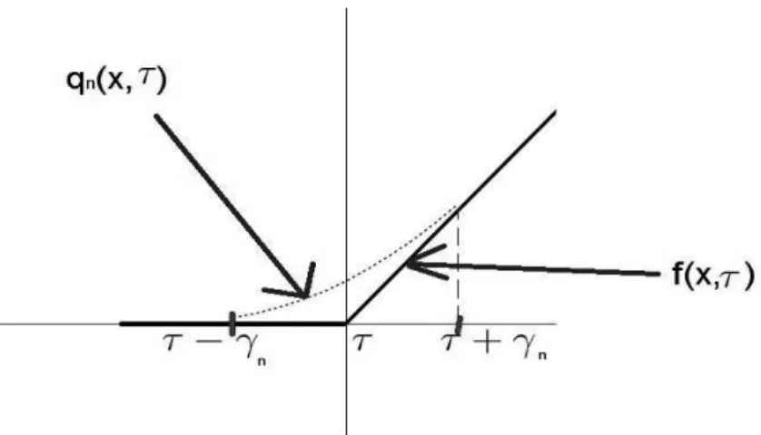
2.1 qn is the smoothed version of f. . . 11
2.2 Mean Square Errors vs log10α for varying sample-sizes with different τ -values, where β0
0 = 0.3, β10 = 1.5, β20 = 1 and σ = 0.5. From the top below, the solid line corresponds to n = 50, dashed line corresponds to n = 100, the dotted line corresponds to n = 500, the dot-dash line corresponds to
n= 1000 and the longdash line corresponds to n= 5000. . . 22 2.3 Co-ordination of primordium initiation and leaf emergence from Spring
Bat-ten treatments resulting in a final leaf number of 8 Brooking and Jameison (2002). The solid bold line represents the one estimated by our approach while the broken line represents the one estimated byBrooking and Jameison (2002). The dotted vertical lines give the confidence intervals for the esti-mated change-points given by the solid lines while the vertical broken-lines indicate the eye-estimated change-points. . . 24 2.4 E2 profile analysis at baseline mean BMI for a non-smoker: the solid line
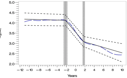
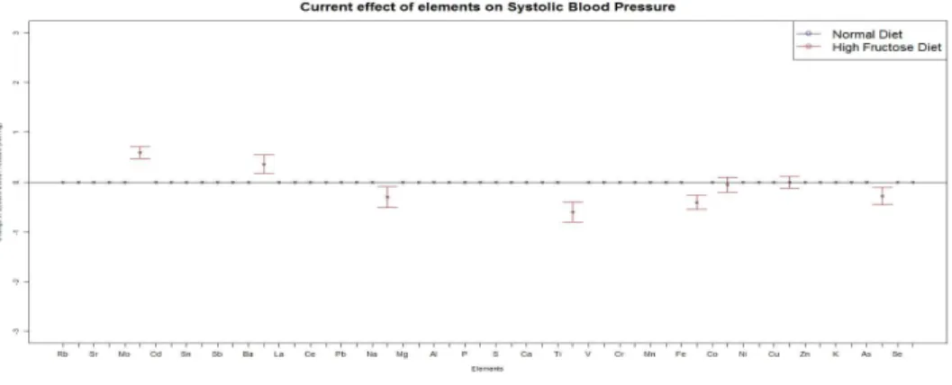
represents the mean estimator using two change-point broken-stick model, the short-broken lines the corresponding pointwise 95% confidence bands; the long-broken lines represent the smooth estimator of the mean function from semiparametric mixed effects model using the same method as in Sow-ers et al. (2008); the shaded regions represent the 95% confidence intervals for the two change-points. . . 27 3.1 Confidence intervals of effects of standardized pollutant concentrations on
Systolic Blood Pressure . . . 38 3.2 Confidence intervals of effects of standardized pollutant concentrations on
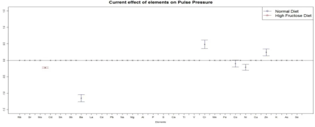
3.3 Confidence intervals of effects of standardized pollutant concentrations on Mean Arterial Pressure . . . 38 3.4 Confidence intervals of effects of standardized pollutant concentrations on
Pulse Pressure . . . 39 3.5 Confidence intervals of effects of standardized pollutant concentrations on
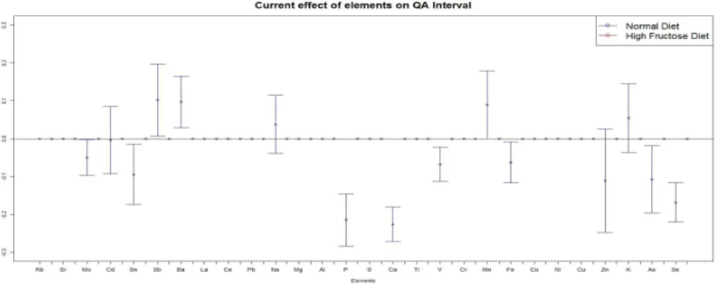
Heart Rate . . . 39 3.6 Confidence intervals of effects of standardized pollutant concentrations on
Temperature . . . 39 3.7 Confidence intervals of effects of standardized pollutant concentrations on
QA Interval . . . 40 A.1 Mean Square Errors vs log10α for varying sample-sizes with different τ
-values, where β0
0 = 0.3, β10 = 1.5, β20 = 1 and σ = 0.5. From the top below,the shortdash-longdash line corresponds to n = 30, the solid line corresponds to n = 50, dashed line corresponds to n = 100, the dotted line corresponds to n = 500, the dot-dash line corresponds to n = 1000 and the longdash line corresponds to n = 5000. . . 79
LIST OF TABLES
Table
2.1 Simulation results comparing the run-times of the existing (Hudson, 1966) and proposed methods for one and two change-point(s) model, with ratio of the time taken by the existing method with respect to that of the proposed one. . . 18 2.2 Bias and variances for the change-point estimate ˆτncompared for one
change-point problem in 3 setups: A:θT = (0.2,1,1,0.6), B:θT= (0.3,1.5,1,0.8) &
C: θT = (0.3,1.5,
−1,0.2) (S.D.: Average of estimated standard deviations over 1000 replications; Emp. S.D. : Sample standard deviation based on 1000 replications). . . 19 2.3 Bias and variances for the change-point estimate ˆτncompared for two
change-points problem in 3 setups: D:θT = (0.3,1,1,1,0.2,0.8), E:θT = (0.2,1,2,1,0.4,0.6)
& F:θT= (0.3,1,
−1,1,0.2,0.8) (S.D.: Average of estimated standard devi-ations over 1000 replicdevi-ations; Emp. S.D. : Sample standard deviation based on 1000 replications). . . 20 2.4 Bias and variances for the change-point estimate ˆτncompared for two
change-points problem in 3 longitudinal setups: G: θT = (0.3,1,1,1,0.2,0.8), H:
θT = (0.2,1,2,1,0.4,0.6) & J: θT = (0.2,1,2,1,0.4,0.6). 10 observations
per individual in set-ups G and H. In set-up J, number of observations per individual D ∼ Discrete Uniform {1,2, . . . ,20}(S.D.: Average of estimated standard deviations over 1000 replications; Emp. S.D. : Sample standard deviation based on 1000 replications). . . 23 2.5 Regression parameter estimates along with their respective standard errors 26 3.1 Simulation results comparing the proposed method with inference method
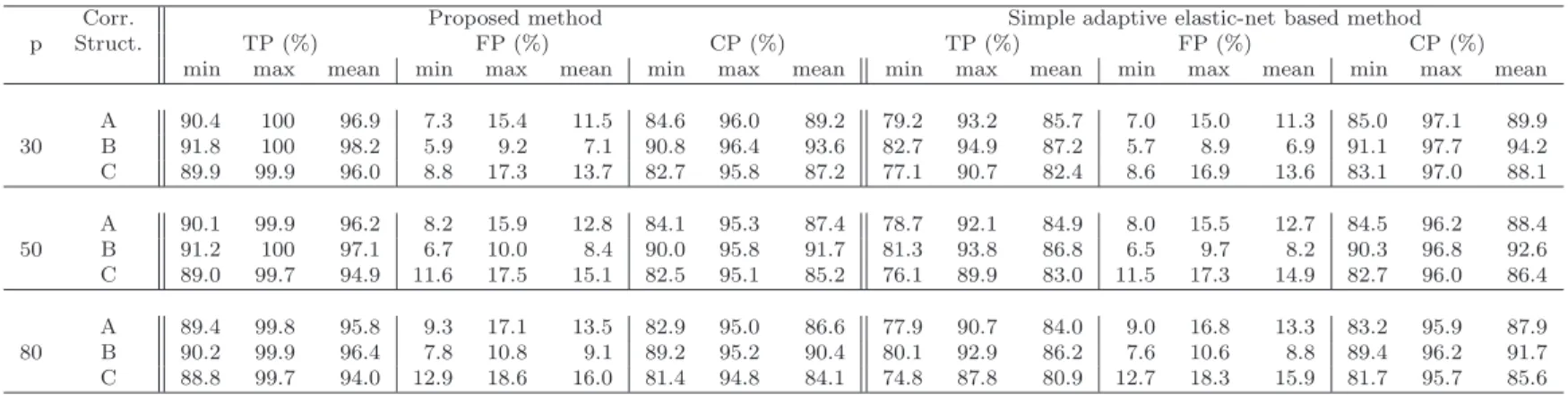
based on simple adaptive elastic-net: min:= minimum over all the co-ordinates, max:= maximum over all the co-ordinates and mean:= mean over all the co-ordinates . . . 43
4.1 Percentage of times the method was able to identify the variable correctly 52 4.2 Bias and standard deviations, in parentheses, of the estimates over 1000
replications for Set-up 1 . . . 52 4.3 Bias and standard deviations, in parentheses, of the estimates over 1000
replications for Set-up 2 . . . 53 4.4 Average bias of the estimates over 1000 replications for Set-up 3 . . . 54 4.5 Distribution (in percentages) of the estimated number of change-points by
ABSTRACT
Efficient Inferential Methods in Regression Models with Change Points or High Dimensional Covariates
by Ritabrata Das
Co-Chairs: Moulinath Banerjee and Bin Nan
This dissertation focuses on providing efficient inferential method for estimation in broken-stick model in cross-sectional as well as longitudinal studies, applying the multivariate adap-tive elastic-net for statistical inference in a multiple pollutant model and proposing a variable selection procedure for multiple change-points in a broken-stick framework.
Estimation of change-point(s) in the broken-stick model has significant applications in modeling important biological phenomena. In the first project, we present a computationally economical likelihood-based approach for estimating change-point(s) efficiently in both cross-sectional and longitudinal settings. Our method, based on local smoothing in a shrinking neighborhood of each change-point, is shown via simulations to be computationally more viable than existing methods that rely on search procedures, with dramatic gains in the multiple change-point case. The proposed estimates are shown to have √n-consistency and asymptotic normality – in particular, they are asymptotically efficient in the cross-sectional setting – allowing us to provide meaningful statistical inference. As our primary and motivating application, we study the Michigan Bone Health and Metabolism Study cohort data to describe patterns of change in log estradiol levels around the final menstrual
period, for which a two change-point broken-stick model appears to be a good fit. We also illustrate our method on a plant growth data set in the cross-sectional setting.
Though there has been a considerable work done on studying the effects of coarse and fine ambient particles, how the constituent pollutants affect cardiovascular functioning is still not clearly understood. In the second project, we propose using the multivariate adaptive elastic-net to capture these effects in a multivariate autoregressive model for time series data. Because of the large number of highly correlated pollutants, a reliable method must take into account the high dimensionality as well as the multicollinearity issues. This is accomplished by using the adaptive elastic-net which deals effectively with the correlated nature of the data during variable selection. Furthermore, the selection consistency and asymptotic normality properties allow us to provide meaningful statistical inference in this set-up. The method is shown to perform well in numerical studies. As our motivating example, we study the effects of multiple pollutants on several cardiovascular end-points in a rat study based in Dearborn, Michigan, conducted by the Great Lakes Air Center for Integrative Environmental Research (GLACIER).
Finally, we look at problems where there are several covariates (large p) and some of the covariates have a simple linear effect while some have a broken-stick effect. In principle, we are looking at two separate but similar types of problems–one where we have several covariates each with possibly a broken-stick effect but with only a single change-point and the other where the broken-stick effect is exhibited in a single covariate but the number of change-points is unknown. In both settings we strive for a parsimonious yet accurate model, which necessitates an effective variable selection procedure. In a sparse setting, we illustrate the difficulty in using the popular variable selection methods and propose a post local-smoothing thresholded ridge regression as a method for identifying the non-zero linear and broken-stick type effects. We illustrate the efficiency of this approach via simulations and discuss possible routes for theoretical justification.
CHAPTER 1
Introduction
A principal task in modern statistics is to provide computationally and theoretically efficient solutions for non-standard regression set-ups. These problems find application in various disciplines of science including medicine, biology, genomics, environmental sciences and economics. Coming up with efficient estimation methods and studying their properties is a major challenge in these settings. One such problem is to devise a computationally fast as well as theoretically viable estimation method for a broken-stick model in both cross-sectional and longitudinal set-ups. This problem is studied in detail in Chapter 2. In Chapter 3, we propose an inference method based on multivariate adaptive elastic-net in a multiple pollutant set-up. Finally, in Chapter 4, an algorithm for variable selection for high dimensional sparse regression, where some of the covariate effects may be of the form of a broken-stick. This thesis covers three main topics. We provide a summary of these topics in the following section.
1.1
Fast efficient estimation method for broken-stick
The Michigan Bone Health and Metabolism Study (MBHMS) is a population-based lon-gitudinal natural history study of ovarian aging conducted in a cohort of White women from the Tecumseh (Michigan) during their young and mid-adulthood years. The goal of Sowers
et al. (2008) was to describe the serum estradiol (E2) profile changes before and after Final Menstrual Period (FMP). Fig. 1 inSowers et al.(2008) indicates that the mean function can be fit nicely by a piecewise linear model with multiple change-points (i.e. the broken-stick model), whose identification is of considerable significance. However, existing methods of change-point estimation in a broken-stick model are fairly slow for large sample sizes. In the particular scenario of Sowers et al. (2008), the effective sample-size is of order of 104 and hence a fast method of estimating the change-point locations precisely and providing corresponding confidence intervals is of considerable importance.
Our method, based on local smoothing in a shrinking neighborhood of each change-point, is shown via simulations to be computationally much faster than existing methods that rely on search procedures. The computational gain gets accentuated in multiple change-points models. The proposed estimates are shown to have√n-consistency and asymptotic normality – in particular, they are asymptotically efficient in the cross-sectional setting (in the sense, they have the same asymptotic distribution as the exact least squares estimate as shown in Feder (1975a) ) – allowing us to provide meaningful statistical inference. We use our prosed estimation method to study the E2 profile, as discussed above.
1.2
High-dimensional Inference based on Multivariate Adaptive
Elastic-net for Multiple Pollutant Data
With advancement in modern technology, high-dimensional regression problems are be-coming more and more common in all disciplines of science. One such interesting problem arises in studying the effects of multiple pollutants on cardio-metabolic end-points. Al-though, the effects of fine particulate matter, as a whole, has been studied in recent years in quite some detail, how the constituent pollutants affect health responses is still up for debate. Two of the major problems in a multiple pollutant regression model is the high-dimensionality and the acute multicollinearity. We propose an inference procedure based on
multivariate adaptive elastic-net in a multivariate autoregressive model for time series data. This method is shown via simulations to effectively address both the major issues with this type of a modeling strategy. We used our method to study the effects of multiple pollutants on several cardiovascular end-points in a rat study based in Dearborn, Michigan, conducted by the Great Lakes Air Center for Integrative Environmental Research (GLACIER).
1.3
Variable selection for high-dimensional broken-stick
regres-sion
This problem is, in some sense, an extension of the problem discussed in 2. Previously, we were interested in estimating the broken-stick model in a fixed dimensional set-up. Now, with high dimensional regression techniques becoming more and more useful, the natural question is how to do variable selection in a usual sparse regression set-up with an added feature – we allow the covariates to have a broken-stick type effect on the response. This problem can be viewed from a very general setting with several covariates each with possibly multiple change-points. But to get a better understanding of the problems at hand, it makes more sense to look at two separate cases:
(i) There are several covariates, each possibly having a broken-stick effect; but we allow the broken-stick to have only one change-point.
(ii) The broken-stick effect is limited to only one covariate but it can have several change-points but the number of change-change-points is unknown
In both set-ups we need to arrive at a parsimonious yet accurate model, which of course necessitates an effective variable selection procedure for these models. Because of the lack of differentiability or restricted strong convexity (Loh and Wainwright, 2015) of the loss function, it is difficult to see how popular variable selection methods will work for this set-up. We propose post local smoothing thresholded ridge regression as a method for variable selection in such a scenario. The method is shown through numerical studies for the first
case to have a very high ability not only to separate signals from noise terms, but also to identify which signals are simply linear and which have a broken-stick type effect.
CHAPTER 2
Fast estimation of regression parameters in a broken
stick model for longitudinal data
2.1
Introduction
In regression models, it is often assumed that the regression function throughout the domain of interest has the same parametric form. But it is also important to consider situa-tions where the regression function has different functional forms in separate porsitua-tions of the domain of interest. A special case of this is the continuous piecewise linear model, popularly referred to as the “broken-stick model”. This model is frequently useful in environmental and biological setups where the locations of the change-points are of interest. The broken-stick with r change-points is E(Y|X, Z) =β0+β1X+ r X k=1 βk+1f(X, τk) +ZTλ, (2.1) where f(x, τ) = (x−τ)+= x−τ, x > τ; 0, x≤τ.
and τj’s are ordered. Such a modelling strategy is of particular interest for the Michigan
MBHMS is a population-based longitudinal natural history study of ovarian aging con-ducted in a cohort of 664 White women from Tecumseh, Michigan during their young and mid-adulthood (24−44) years. Sowers et al. (2008) studied the serum estradiol (E2) hor-mone levels in 629 women enlisted in the MBHMS over a fifteen year period starting from 1992. The goal ofSowers et al.(2008) was to describe the E2 profile changes before and after Final Menstrual Period (FMP). A semiparametric mixed model approach was implemented inSowers et al. (2008), and smoothing splines were used for estimation. Referring to Fig. 1 in Sowers et al. (2008), it is clear that the mean function can be fit nicely by a piecewise linear model with multiple change-points, whose identification is of considerable significance. However, existing methods of change-point estimation in a broken-stick model are fairly slow for large sample sizes. In the particular scenario ofSowers et al.(2008), the effective sample-size is of order of 104 and hence a fast method of estimating the change-points precisely is of considerable importance.
In the early literature, it was generally assumed that either the exact location of the change-point τ is known (Poirer, 1973), or, at worst, it is known which two observation points τ should lie between (Robinson, 1964). Also, most of the early work focused on detection of whether a change-point existed at all. In this article, however, the existence of change-point(s)is assumed and the exact number of change-points, denoted by r, is assumed known. The focus here is to propose a quick estimation procedure that gets around the non-smoothness of the model without compromising asymptotic efficiency in the process.
The principal difficulty in the estimation problem arises when the locations of the change-points are unknown. For an independent and identically distributed error case, if the location of these change-points were known, we would have a standard linear regression problem. Even if a relatively small set of plausible values were known, one could perform least squares for the slope and intercept parameters for each of these plausible values to find the overall least squares estimate. However, in most scenarios, this is unlikely, and the set of plausible values over which one needs to search is typically all r tuples of ordered Xi’s, leading to a
very high number of linear regressions, nr
in principle, n being the sample size; see Hudson (1966).
Bellman and Roth (1969) proposed an alternative method based on dynamic linear pro-gramming but this method is even slower than the previous method. Feder (1975b) con-sidered a general case of segmented regression problems and showed that the exact least squares estimate obtained byHudson (1966) is asymptotically normal. In particular, for the broken-stick model, the estimate is √n– consistent.
Tishler and Zang (1981) were the first to suggest estimation of change-points using a max-imum likelihood approach based on smoothing. They argued that the non-differentiability of the ‘maximum’ and ‘minimum’ operators in piecewise regression was the main problem in using maximum likelihood. However, if these operators were substituted by smoothed versions, maximum likelihood could readily be used for fast computation. Tishler and Zang (1981) suggested using a quadratic approximation, where the length of the interval on which
f is smoothed was taken as an arbitrary small value. However, the behavior of these esti-mates, as the interval-length shrinks to 0, was not investigated. It is clear that unless the length of the interval is allowed to decrease with sample size, their algorithm cannot yield a consistent estimate.
Recent articles for broken-stick models include Bhattachaya (1987),Huskova (1998) and Muggeo (2003). While the first two deal with theory, Muggeo (2003) tries to develop an estimation strategy, but does not provide any asymptotic results and thus fails to address the theoretical efficiency of the approach. For a detailed description of Bayesian methods of change-point estimation refer to Chen et al.(2011).
In sum, the lack of a suitable method of estimation, that is optimal in terms of both precision and computational economy, has forced statisticians to fall back on the search-based algorithm of Hudson or related algorithms thereof. Our paper fills this gap in the literature.
have also been investigated. Chiu et al. (2006) suggested that in certain scenarios, instead of using the broken-stick as the true model, it might be better to use, what they referred to as, the “bent-cable model”, which is a quadratic smoothing of the broken-stick model in a γ
neighborhood around τ. Their change-point parameter was defined as the mid-point of the interval (τ −γ, τ +γ) on which the smoothing was done; here both τ and γ are unknown parameters. It was shown that ˆτn, the least squares estimate ofτ, is√n– consistent. Also, for
γ0 >0, ˆγn is √n-consistent as well. In a previous article, Chiu et al. (2002) had shown that
for γ0 = 0, i.e., when the smooth model reduces to the broken-stick model, the asymptotics are complex and ˆγn is at most n1/3– consistent.
In this chapter, equation (2.1) is used as the true mean model. Ideally, one would want to minimize the residual sum of squares in this model by a Newton-Raphson type algorithm, but this is not viable owing to the non-differentiability off atτ. To this end, we use a twice differentiable perturbation of f, denoted by qn, as our working model, where qn coincides
with f outside a shrinking neighborhood of τ, say (τ−γn, τ+γn), with γn, a user-specified
tuning parameter, going to 0. Because qn is differentiable, the minimization can be done by
Newton’s algorithm very quickly. For the iid error case, we show that our estimate of τ is indeed √n– consistent for τ, and furthermore has an asymptotic normal distribution with the same asymptotic variance as the exact least squares estimate of Hudson (1966). For the longitudinal model, the same method yields √n–consistent and asymptotically normal estimates for the change-points even for misspecified variance structures.
In sections 2.2 and 2.3, we introduce the model for both the cross-sectional and longitu-dinal set-ups respectively and outline the main steps of the estimation. The main theoretical results are presented along with the main ideas of the proofs. Section 2.4 contains simulation results indicating the efficiency of the proposed method while the method is applied to two real data —plant growth data (cross-sectional study) in section 2.5.1 and estradiol profile analysis (longitudinal study) in section 2.5.2. Proofs are provided in Appendix A.
2.2
Cross-sectional Study
We assume that the covariate X is contained in [M1, M2]. The regression parameter in the cross-sectional set-up (2.1), is denoted by θT = (βT, τT, λT). We assume θ belongs to a
compact set Θ =B×[M1+δ, M2−δ]r×Λ,τ
k< τk+1, k= 1,2..., r−1, and|M1|,|M2|<∞and
δ is a known small positive constant, indicating the change-points need to be well-separated from the boundaries of theX−space. Without loss of generality, takeM1 = 0 and M2 =M. We write βT = (β
0, β1, ..., βr+1) ∈ B, where β0 is the intercept and Pkj=1βj is the slope of
the kth segment, k = 1,2..., r + 1. B is a compact set in Rk+2; the restriction ζ ≤ β
k ≤ B,
2≤k≤r+ 1 is imposed for the sake of identifiability. We also writeτT = (τ
1, τ2, ..., τr), with
τk denoting the k’th smallest change-point, and again identifiability requires the conditions
τk< τk+1, k = 1,2..., r−1,τ1 ≥δ and τr ≤M −δ. Λ is assumed to be a compact set in Rl.
The errors εi are assumed to be independent and identically distributed with mean 0 and
variance σ2. The true parameter vector θ0 = (β0
0, β10, ..., βr0+1, τ10, τ20, ..., τr0, λ0)T is assumed
to be an interior point of the compact set Θ. Our data are independent and identically distributed observations {Yi, Xi, Zi}ni=1 from (2.1) and henceforth, Pn denotes the empirical
measure of the data. Note that, Yi and Xi are scalars while Zi is an l−dimensional vector
of covariates with no change-points.
2.2.1 Estimation Define, M(θ, x, y, z) = (y−Eθ(Y|X=x, Z =z))2 = " y− ( β0+β1x+ r X k=1 βj+1f(x, τk) +zTλ )#2 .
The exact least squares procedure aims to obtain the minimizer of
Pn(M(θ, X, Y, Z)) = 1 n n X i=1 M(θ, Xi, Yi, Zi).
Asf(x, τ) is not differentiable atτ, one cannot obtain the minimizer ofPn(M(θ, X, Y, Z))≡ Pn(M(θ)) (for notational convenience) by Newton’s algorithm. So, we resort to minimize Pn(Mn(θ)), where Mn(θ)≡Mn(θ, x, y, z) = [y− {β0+β1x+ r X k=1 βj+1qn(x, τk) +zTλ}]2
isour working model, a smoothed approximation ofM(θ). Basically each of the f’s inM(θ) is replaced by its corresponding smoothed version qn to obtain Mn(θ).
As far as the functional form ofqnis concerned, the motivation lies in the work ofTishler
and Zang (1981) andChiu et al.(2006). Tishler and Zang (1981) suggested using a quadratic approximation, where the length of the interval on which f is smoothed was taken as an arbitrary small value, while Chiu et al. (2006) considered the length of the corresponding interval as a parameter. We consider the same functional form for qn as in these papers,
but in our model, the length of the interval on which we smooth f is a user-specified tuning parameter shrinking to 0 with n at an appropriate rate as n → ∞. More specifically,
qn(x, τ) = 0, if x < τ −γn; (x−τ+γn)2 4γn , if τ −γn≤x≤τ +γn; (x−τ), if x > τ +γn; (2.2)
where γn is a deterministic sequence, that approaches zero asn → ∞.
Define ˆθn = arg minθ∈ΘPn(Mn(θ)). In Appendix A.1, we show that ˆθn is a zero of the
surrogate empirical estimating functionUn(θ) =∂Pn(Mn(θ))/∂θ, with probability increasing to 1, validating the use of the solution of Un(θ) as our numerical estimate. It is not clear whether this zero is unique but this is not an issue, since for our asymptotics, how we pick the minimizer is immaterial, meaning that the results hold true for any choice of zero of Un(θ). Our numerical results, however, suggest that generally there is a unique minimizer.
Figure 2.1: qn is the smoothed version of f.
2.2.2 Asymptotic Results
For model (2.1) we consider the following regularity conditions.
Condition 1.1: There are r distinct change-points τ1, . . . , τr in model (2.1) for a fixed
integer r≥1; r is known.
Condition 1.2: Covariate X ∈ [0, M], M < ∞, follows a continuous distribution FX
such that pr(τk < X ≤ τk+1) > 0, k = 0, . . . , r with τ0 = 0 and τr+1 = M. The joint distribution of Z is denoted by FZ.
Condition 1.3: Changes of slope parameters satisfy 0 < ζ ≤ |βk| ≤ B < ∞, k =
2,3, . . . , r+ 1, for some constants ζ and B.
Theorem 2.1. Under Conditions 1.1-1.3, θˆn is a consistent estimator forθ0 for any
deter-ministic sequence γn→0 as n→ ∞.
The proof of Theorem 2.1 is based on the argmax (argmin) continuous mapping theorem (van der Vaart and Wellner, 1996). First, we show that θ0 is the unique minimizer of
P(M(θ)) in Θ. then, it suffices to show that kPn(Mn)−P(M)k := supθ
∈Θ|Pn(Mn(θ))−
P(M(θ))| = op(1); here P f =
R
f dP, P being the probability measure that generates the data. For the case with a single change-point and covariate Z absent, the proof is presented
in Appendix A.1. The proof for the case with multiple change-points or with other covariates is an exercise involving extensive algebraic derivations following the same line. Note that, in Appendix A.1, we also prove that θ0 is the unique solution ofU(θ) =∂P(M(θ))/∂θ = 0, which implies that the estimate obtained by Newton-Raphson of the smoothed score equation converges to the trueθ0, and not to some local minima.
Theorem 2.2. Forγn=n−α withα >1/2, under Conditions 1.1-1.3, we have thatn1/2(ˆθn−
θ0)converges in distribution to a normal random variable with mean0and covariance matrix 2σ2U˙−1
∗ (θ0). The kl-th element of matrix U˙∗ is ( ˙U∗(θ0))kl = 2P(HT(θ0)H(θ0)), where
H(θ) = 1, X, f(X, τ1), . . . , f(X, τr), −β21(X > τ1), . . . ,−βr+11(X > τr), Z
1×(2+2r+l). The proof of Theorem 2.2 also consists of two major steps. To this end, let us define
θn as the minimizer of P(Mn(θ)) in Θ closest to θ0. The first step is to show that θn
converges to θ0 with a faster than √n rate, which in fact is γ
n, and the second to show
the asymptotic normality ofn1/2(ˆθ
n−θn). Both steps rely on Taylor series expansions. For
notational simplicity, we provide the proof for the case with single change-point and absence of Z in Appendix A.2. The case with multiple change-points and other covariates is again a straightforward extension.
The following Corollary shows that our proposed local smoothing method does not lose any efficiency. Its proof is provided in Appendix A.3.
Corollary 2.3. The asymptotic distribution of our estimate, as stated in Theorem 2.2, is exactly the same as that in Feder (1975a) for the exact least squares estimate in the broken stick model.
Remark 2.4. Please note that for the sake of notational convenience and to keep the results and proofs terse, only one variable with change-points have been included in model (2.1). However, the method will work equally well for a model consisting of multiple variables, with
multiple change-points in each variable, and the results will be analogous.
2.3
Longitudinal study
The model for the longitudinal study with a broken-stick mean function is
E(Yij|Xij, Zi) =µij =β0+β1Xij + r
X
k=1
βk+1f(Xij, τk) +ZiTλ, (2.3)
where Yij is the response of the ith subject at the jth time-point (tij) and Xij denotes
the corresponding covariate with r change-points, while Zi are l time-invariant covariates,
j = 1, . . . , mi , i= 1, . . . , n.
For the regression parameters, βT = (β
0, β1, .., βr+1), we have the same assumptions as in
the cross-sectional model. We assume the effect sizes λ ∈ Λ (a compact set in Rl) and τ is
the vector of change-points, as before. Here, θT = (βT, τT, λT) is our parameter of interest and θ0 is the true value ofθ.
As far as the variance function is concerned, we postulate the following form:
Cov(Yij, Yik) = g(η, tij, tik), (2.4)
Cov(Yij, Ylk) = 0, i6=l;j, k = 1, . . . , mi;i= 1, . . . , n,
where η is the vector of covariance parameters. We assume that the observations across individuals are independent and the correlation between different observations of the same individual can depend on the time-points but not on the mean parameters, θ.
Yi is used to denote the vector of mi observations for the i−th individual, i = 1, . . . , n.
Y = (Y1, . . . , Yn) is the vector of all responses. We use similar definitions for Xi and X. Let
Σ(i)denote the dispersion matrix ofY
i and Σ the dispersion matrix ofY. The true dispersion
matrix is denoted by Σ0, which can be written as Σ(η0), η0 being the true value of η. To establish the asymptotic results rigorously, the problem needs to be cast in a proper
mathematical framework. We assume that, the number of repeated measures is denoted by the random variableDwhich takes values in the integer-space{1,2, . . . , L}with probabilities
p1, p2, . . . , pL respectively. Note that this L is assumed fixed and known. Also we have a
triangular array of X-values,
X1(1) X1(2) X (2) 2 X1(3) X2(3) X3(3) ... . .. X1(L) X2(L) X3(L) . . . XL(L).
When D =d, the d-th row of this array is selected as the set of time-dependent covariates. The same is true for the measurement errors {εij}and they are assumed to be independent
of {Xij}’s. Thus, Y(D) =β0+β1X(D)+ r X k=1 βk+1f(X(D), τk) +ZTλ+ε(D) =µ(D)+ε(D).
The observation for each individual consists of (D, Y(D), X(D), Z) and our data comprise of
n iid copies of this array. As with most inference methods in longitudinal studies, we allow for ignorable dropouts (Rubin, 1976).
2.3.1 Estimation
The estimation process is divided into three steps:
Step 1 : Assume working independence, i.e. take Σ(i) = I, i = 1, . . . , n. As for the cross-sectional study, replace each of thef’s by their respective smoothed versionqn’s. Now,
find the corresponding estimate ˆθn(I) as the solution to the estimating equation
∂ ∂θPn[(Y
(D)
where µ(nD) is the smoothed version of µ(D).
Step 2 : Then use ˆθn(I) to estimate the nuisance parameter η. The specifics will depend
on the nature of the covariance function g in (2.4).
Step 3 : Use ˆηn obtained in step 2 to estimate θ. So the final ˆθn is the solution to the
estimating equation ∂ ∂θPn[(Y (D) −µ(nD))TΣˆ−n1(Y(D)−µ(nD))] = 0, where ˆΣ−1
n is the block-diagonal dispersion matrix based on ˆηn .
2.3.2 Asymptotic Results
As in the cross-sectional model, for the longitudinal model we consider similar regularity conditions.
Condition 2.1: There are r distinct change-points τ1, . . . , τr in model (2.3) for a fixed
integer r≥1; r is known.
Condition 2.2: Conditional on D = d, covariate X ∈ [0, M]d, M < ∞, follows a
continuous distribution FX such that pr(τk < Xj ≤ τk+1) > 0, for some j = 1, . . . , d, for all k = 0, . . . , r with τ0 = 0 and τr+1 =M. Also we assume the covariates Z follow a joint distribution FZ.
Condition 2.3: Changes of slope parameters satisfy 0 < ζ ≤ |βk| ≤ B < ∞, k =
2,3, . . . , r+ 1, for some constants ζ and B.
Condition 2.4: There exists a positive definite matrix W, such that estimated covari-ance matrix ˆΣn satisfies √n( ˆΣn−W) = Op(1).
Theorem 2.5. Under Conditions 2.1-2.4,
(a) The estimator θˆn is consistent for θ0 given any deterministic sequence γn → 0 as
(b) For γn = n−α with α > 1/2, n1/2(ˆθn −θ0) converges in distribution to a normal
random variable with mean 0 and covariance matrix
K(W−1) = 2 L X d=1 P(d)[(HT(θ0)W−1H(θ0))−1(W−1H(θ0))TΣ0(W−1H(θ0)) (HT(θ0)W−1H(θ0))−1]pd where H(θ) = 1 X f(X, τ1) . . . f(X, τr) −β21(X > τ1) . . . −βr+11(X > τr) Z d×(l+2r+2); here P(d)f = R
f dP(d), P(d) being the probability measure that generates the data given
D=d.
Remark 2.6. If the matrix W in condition 2.4 is indeed the true covariance matrix Σ0, i.e., ˆ
Σnis a√n-consistent estimate of Σ0, then forγn=n−α withα >1/2,n1/2(ˆθn−θ0) converges
in distribution to a normal random variable with mean 0 and covariance matrix
K(Σ−1 0 )= 2 L X d=1 P(d)[(HT(θ0)Σ0−1 H(θ0))−1]pd.
The proof of Theorem 2.5 is similar to the proofs of Theorems 2.1 and 2.2 in Section 2.2. The main proof is divided into three major parts. First, we show that√n(ˆθn(I)−θ0) converges
toN(0, K(I)) in distribution. Next, we prove √n(ˆθ(W−1)
n −θ0) converges to N(0, K(W−
1)
) in distribution. Here, ˆθn(W−1) is defined as the minimizer ofPn(Y −µn)TW−1(Y −µn), which is
shown to be a zero ofU(nW−1)(θ) = ∂
∂θPn(Y −µn)TW−1(Y −µn), with probability increasing
to 1. Finally, we show that√n(ˆθn−θˆ(W
−1)
n ) = op(1),which proves Theorem 2.5.
For the sake of notational convenience, the proof is presented in Appendix A.4, forr = 1 and for fixed visit-times, i.e. D ≡ m or equivalently mi = m for all i = 1, . . . , n. Also for
Though the proof provided in Appendix A.4 is for a fixed number of visit-times, it holds true for variable number of visit-times, as stated in Theorem 2.5. Notice that, conditional on
D=d(this event has probabilitypd), it is shown that n1/2(ˆθn−θ0) converges in distribution
to a normal random variable with mean 0 and covariance matrix
K(W−1)
= 2P(d)[(HT(θ0)W−1H(θ0))−1(W−1H(θ0))TΣ0(W−1H(θ0)) (HT(θ0)W−1H(θ0))−1].
Now, the result of Theorem 2.5 easily follows.
Corollary 2.7. Denoting the mean function at X = x, Z = z by µ(x, z, θ), we have √
n(µ(x, z,θˆn)−µ(x, z, θ0))converges in distribution to a normal random variable with mean
zero and variance aTK(W−1)
a, where
aT = (1, x, f(x, τ10), . . . , f(x, τr0),−β201(x > τ10), . . . ,−βr0+11(x > τr0), z)
.
This result is useful in providing pointwise confidence bands for the broken-stick mean function as illustrated in Fig 2.4. The proof is provided in the Appendix A.8
Remark 2.8. Note that the estimated confidence band for the mean at ˆτn, as provided by
Corollary 2.7 is discontinuous. The asymptotic distribution of√n(µ(ˆτn, z,θˆn)−µ(τ0, z, θ0))
is not a direct application of this result, but needs separate calculations —a direct application of the delta method.
2.4
Simulations
2.4.1 Cross-sectional set-up
Simulations were conducted to compare the proposed method with the existing one. Models with one and two change-points were both considered. Sample sizes were varied,
n = 50,200,1000,5000. For each of the two models, for a fixed n, 3 different sets of values of θ were considered within the domain of interest. For each value of θ, the proposed and existing (Hudson, 1966) methods were both repeated N = 1000 times. The run-times, a measure of computational efficiency, for each of the methods were then averaged over these 1000 repetitions and over the 3 different values of θ. This was done to average out discrepancies being caused by individual θ’s. Error standard deviation σ was taken to be equal to 0.1 for all cases and M = 1. For all simulations, α was taken to be 1. The simulations were carried out on an Intel(R) Core(TM) i7 system with 1.6 GHz and 8 GB RAM in a 64-bit OS.
2.4.1.1 Results
Table 2.1: Simulation results comparing the run-times of the existing (Hudson, 1966) and proposed methods for one and two change-point(s) model, with ratio of the time taken by the existing method with respect to that of the proposed one.
Sample Mean Time (Seconds)
Sizen One change-point Two change-points Existing Proposed Ratio Existing Proposed Ratio
50 0.18 0.006 30 2.36 0.02 118
100 0.30 0.008 38 13.86 0.03 462
500 0.97 0.02 49 64.87 0.06 1015
1000 1.89 0.03 63 947.03 0.08 11838
5000 4.98 0.06 83 22843 0.20 114215
From Table 2.1, it is obvious that the proposed method is much faster than the exact least squares method, especially for two change-point problems. Also Tables 2.2 & 2.3 indicate that the change-point estimates of the proposed method are almost as accurate as the exact least squares estimate. The biases are close to zero for all sample sizes, especially for the large
Table 2.2: Bias and variances for the change-point estimate ˆτn compared for one
change-point problem in 3 setups: A: θT = (0.2,1,1,0.6), B: θT = (0.3,1.5,1,0.8) & C:
θT = (0.3,1.5,
−1,0.2) (S.D.: Average of estimated standard deviations over 1000 replications; Emp. S.D. : Sample standard deviation based on 1000 replications).
Sample Bias (S.D., Emp. S.D.) Theoretical
Size ×10−3 S.D. n Existing Proposed ×10−3 Set-up A 50 -8.2 (58.1, 60.3) -12.4 (58.3, 61.0) 57.8 100 -4.3 (41.0, 41.2) -5.2 (41.0, 41.3) 40.9 500 -2.1 (18.3, 18.4) -2.9 (18.3, 18.5) 18.3 1000 -0.6 (12.9, 12.9) -0.9 (12.9, 13.0) 12.9 5000 -0.0 (5.8, 5.8) -0.1 (5.8, 5.8) 5.8 Set-up B 50 -9.2 (71.6, 73.2) -14.1 (71.6, 73.6) 70.7 100 -4.7 (50.1, 50.3) -5.9 (50.1, 50.4) 50.0 500 -2.8 (22.4, 22.4) -3.3 (22.4, 22.5) 22.3 1000 -0.9 (15.8, 15.8) -1.2 (15.8, 15.8) 15.8 5000 -0.1 (7.1, 7.1) -0.1 (7.1, 7.1) 7.1 Set-up C 50 8.1 (71.6, 73.3) 12.8 (71.6, 73.5) 70.7 100 4.7 (50.1, 50.4) 6.2 (50.1, 50.5) 50.0 500 1.8 (22.4, 22.4) 2.0 (22.5, 22.6) 22.3 1000 0.2 (15.8, 15.8) 0.4 (15.8, 15.8) 15.8 5000 0.1 (7.1, 7.1) 0.1 (7.1, 7.1) 7.1
samples. The standard deviation estimates are very close to the sample standard deviations indicating our standard deviation estimates work well, especially for large samples. The estimates are also very close to the theoretical standard deviations, indicating the asymptotic efficiency of our estimates. Although the bias and variances for the β’s have not been tabulated for the sake of brevity, we observed that our β estimates also have comparable Mean Squared Errors to their respective exact least squares estimates.
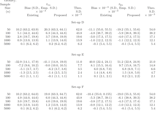
Table 2.3:Bias and variances for the change-point estimate ˆτn compared for two change-points problem in 3 setups: D: θT = (0.3,1,1,1,0.2,0.8), E: θT = (0.2,1,2,1,0.4,0.6) &
F: θT = (0.3,1,
−1,1,0.2,0.8) (S.D.: Average of estimated standard deviations over 1000 replications; Emp. S.D. : Sample standard deviation based on 1000 replica-tions).
Sample ˆτ1n τˆ2n
Size Bias (S.D., Emp. S.D.) Theo. Bias×10−3(S.D., Emp. S.D.) Theo.
(n) ×10−3 S.D. ×10−3 S.D.
Existing Proposed ×10−3 Existing Proposed ×10−3
Set-up D 50 10.2 (63.2, 63.9) 20.3 (63.3, 64.1) 62.0 -11.1 (55.0, 55.5) -19.2 (55.1, 55.6) 54.0 100 5.1 (44.2, 44.6) 6.3 (44.3, 44.8) 43.8 -4.8 (38.7, 39.2) -5.9 (38.8, 39.3) 38.2 500 2.8 (19.7, 19.8) 3.7 (19.8, 19.9) 19.6 -3.0 (17.3, 17.5) -4.0 (17.3, 17.5) 17.1 1000 0.9 (13.9, 13.9) 1.1 (13.9, 14.0) 13.9 -1.0 (12.2, 12.3) -1.1 (12.2, 12.3) 12.1 5000 0.1 (6.2, 6.2) 0.2 (6.2, 6.2) 6.2 -0.1 (5.4, 5.5) -0.1 (5.4, 5.5) 5.4 Set-up E 50 -32.9 (14.1, 17.9) -41.1 (14.8, 19.0) 11.0 40.0 (22.4, 24.1) 51.2 (22.8, 24.9) 21.0 100 -7.2 (9.6, 10.2) -9.0 (10.0, 10.5) 7.7 8.1 (15.5, 16.4) 9.7 (15.8, 16.7) 14.8 500 -5.1 (3.7, 3.7) -6.2 (3.7, 3.8) 3.5 6.0 (6.8, 7.0) 6.8 (6.9, 7.1) 6.6 1000 -1.3 (2.5, 2.5) -1.4 (2.5, 2.5) 2.4 1.4 (4.8, 4.8) 1.5 (4.8, 5.0) 4.7 5000 -0.1 (1.1, 1.1) -0.1 (1.1, 1.1) 1.1 0.1 (2.1, 2.1) 0.2 (2.1, 2.2) 2.1 Set-up F 50 10.2 (63.2, 64.0) 19.8 (63.3, 64.7) 62.0 -10.4 (55.0, 0.155) -19.0 (55.3, 55.8) 54.0 100 4.9 (44.0, 44.6) 6.0 (44.3, 44.8) 43.8 -5.3 (38.7, 39.1) -6.1 (38.8, 39.3) 38.2 500 3.0 (19.7, 19.8) 4.0 (19.8, 19.9) 19.6 -3.8 (17.2, 17.5) -4.3 (17.3, 17.4) 17.1 1000 0.9 (13.9, 14.0) 1.2 (13.9, 14.0) 13.9 -0.8 (12.1, 12.2) -1.0 (12.2, 12.3) 12.1 5000 0.1 (6.2, 6.2) 0.1 (6.2, 6.2) 6.2 -0.1 (5.4, 5.5) -0.1 (5.4, 5.5) 5.4
2.4.1.2 Choice of α for finite samples
Although asymptotic results were established for all α >1/2, what a proper choice of α
should be for finite samples is a very pertinent question. We performed extensive simulations for different sample-sizes, to explore the robustness of different choices of α values.
We tried a sample situation with one change-point, β0
0 = 0.3, β10 = 1.5, β20 = 1 and
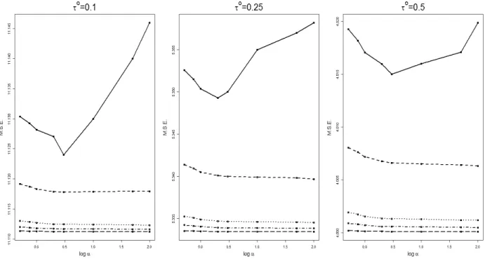
σ = 0.1 with covariate X-space = [0,1]. The τ-values were varied between 0 and 1 and the Mean Square Errors were plotted against log10α values for various sample-sizes. We found that the M.S.E. vs log10α graphs are almost invariant with changing sample-sizes. To change the signal-to-noise ratio, the β-values were kept constant but σ was changed to 0.5 (Fig.2.2) and 1. The patterns are exactly similar for all parameter values and
signal-to-noise ratios. However, for a small n and a very large value ofα, the algorithm occasionally breaks down because ˙Un(θ) becomes (almost) singular for computational purposes. This is clearly indicated by the very large average MSE for α = 50 or 100 when sample-size is small (n= 50). So, very large α’s (greater than 10) are not recommended for small samples (less than 50).We would also like to point out the robustness of the M.S.E.’s to the choice of tuning parameter in the range of α’s for which the algorithm is numerically stable. This is reflected by the flat stretch of the M.S.E. curves for each n, before numerical instability sets in. In other words, so long as the algorithm works, any choice of α > 1/2 is essentially as effective as any other. So, searching for an optimal α is unlikely to yield any significant gains. Our recommendation is to use α= 1, which works very well in terms of M.S.E. for all sample-sizes, as low as 30. The sameαvalue (1) is used for all data anlyses in the subsequent sections. The simulations indicate that computational efficiency is insensitive to the choice of α. A more detailed version of Fig.2.2 is provided in Appendix A.6.
2.4.2 Longitudinal set-up
Simulations were conducted for the longitudinal case as well to compare the efficiency of our proposed method to the search-based algorithm. We considered an AR(1) correlation structure withρ= 0.6 to model the dependence among observations within subject. For each subject, we considered 10 observations in scenarios G and H (Table 2.4). For set-up J, we considered varying number of observations for each individual, which is uniformly distributed over integer-space {1,2, . . . ,20}. Error standard deviation σ was taken to be equal to 0.1 for all cases and M = 1. For all simulations, α was taken to be 1. The computational efficiency of our proposed method is huge compared to the search-based algorithm, as in the cross-sectional case (Table 2.1). So, in Table 2.4, we have just compared the bias and standard errors to illustrate the validity and estimation efficiency of our method.
Results from Table 2.4, clearly indicate that our method yields almost the same standard error estimates as the search-based algorithm. Although for both methods with small
sample-Figure 2.2: Mean Square Errors vs log10α for varying sample-sizes with different τ-values, where β0
0 = 0.3, β10 = 1.5, β20 = 1 and σ = 0.5. From the top below, the solid line corresponds to n = 50, dashed line corresponds to n = 100, the dotted line corresponds to n = 500, the dot-dash line corresponds to n = 1000 and the longdash line corresponds to n= 5000.
sizes, the bias is comparatively high and the standard deviation estimates are higher than the theoretical values, the differences become smaller for larger sample sizes. The M.S.E.’s for the slope and intercept parameters also behave similar to those of the change-points.
2.5
Applications
2.5.1 Plant growth data analysis
Vernalization, a requirement for plants to experience a period of cool conditions to accel-erate flowering, is an important determinant of flowering date in winter wheat. In Brooking and Jameison (2002), controlled environment studies were carried out to quantify the re-sponse of vernalization rate to temperature for two near-isogenic lines of the wheat cultivar
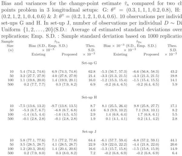
Table 2.4:Bias and variances for the change-point estimate ˆτn compared for two change-points problem in 3 longitudinal setups: G: θT = (0.3,1,1,1,0.2,0.8), H: θT =
(0.2,1,2,1,0.4,0.6) & J:θT= (0.2,1,2,1,0.4,0.6). 10 observations per individual in
set-ups G and H. In set-up J, number of observations per individual D ∼ Discrete Uniform {1,2, . . . ,20}(S.D.: Average of estimated standard deviations over 1000 replications; Emp. S.D. : Sample standard deviation based on 1000 replications).
Sample τˆ1n τˆ2n
Size Bias (S.D., Emp. S.D.) Theo. Bias×10−3(S.D., Emp. S.D.) Theo.
(n) ×10−3 S.D. ×10−3 S.D.
Existing Proposed ×10−3 Existing Proposed ×10−3
Set-up G 10 5.4 (74.2, 74.6) 6.9 (74.3, 74.8) 62.8 -5.3 (56.7, 57.3) -6.6 (56.8, 58.3) 43.2 50 3.2 (27.7, 27.9) 4.0 (27.8, 27.9) 21.4 -3.3 (21.3, 21.5) -4.3 (21.3, 21.5) 19.8 100 1.1 (19.8, 20.0) 1.4 (19.9, 20.1) 16.0 -1.2 (15.3, 15.4) -1.5 (15.4, 15.5) 14.1 500 0.2 (7.7, 7.7) 0.3 (7.9, 8.2) 6.9 -0.2 (6.4, 6.5) -0.2 (6.4, 6.5) 5.9 Set-up H 10 -7.5 (13.6, 13.2) -9.7 (13.8, 13.5) 8.7 8.1 (25.5, 26.4) 9.8 (25.8, 27.7) 17.1 50 -5.3 (6.7, 6.7) -6.8 (6.7, 6.8) 4.6 6.3 (9.9, 10.2) 7.1 (9.8, 10.1) 8.2 100 -1.4 (4.5, 4.4) -1.6 (4.5, 4.5) 2.9 1.4 (6.8, 6.4) 1.7 (6.8, 6.1) 5.5 500 -0.1 (2.8, 2.8) -0.1 (2.8, 2.8) 1.9 0.1 (4.1, 4.1) 0.2 (4.1, 4.2) 2.8 Set-up J 10 5.8 (77.1, 77.6) 7.1 (77.2, 77.8) 64.4 -6.1 (57.7, 59.4) -6.8 (57.2, 59.1) 44.1 50 3.5 (28.5, 28.7) 4.1 (28.5, 28.7) 22.9 -3.9 (22.0, 22.2) -4.4 (21.8, 22.0) 20.6 100 1.2 (20.3, 20.6) 1.4 (20.4, 20.6) 16.6 -1.3 (15.7, 15.8) -1.5 (15.8, 15.9) 14.9 500 0.2 (7.9, 8.0) 0.3 (8.0, 8.2) 7.2 -0.2 (6.8, 6.9) -0.2 (6.8, 6.9) 6.4
Batten: Spring Batten, vernalization insensitive; and Winter Batten, vernalization sensitive. Plants were sampled for dissection at intervals during the treatment and post-treatment pe-riod, until the flag leaf could be distinguished. The authors investigated the co-ordination of primordium initiation and leaf appearance, quantified by the Haun stage. The authors observed that Spring Batten plants grown under fully inductive conditions, 25/20oC, 16 hrs photoperiod, produced eight leaves on average, and the rate of primordium initiation per emerged leaf increased markedly with the transition from leaf initiation to spikelet initiation. This represents an important phase transition in the growth of the plant. From Fig. 2.3, it is quite clear that the model which best fits the scenario is a broken-stick model with two change-points. The authors had estimated the change-points by naked eye and then fitted three line-segments for the three regions. We provide a fast as well as statistically rigorous
analysis using the approach developed in this paper. 0 1 2 3 4 5 6 7 8 9 0 5 10 15 20 25 30
Modified Haun stage
Cumulative primordia
Figure 2.3: Co-ordination of primordium initiation and leaf emergence from Spring Batten treatments resulting in a final leaf number of 8 Brooking and Jameison (2002). The solid bold line represents the one estimated by our approach while the broken line represents the one estimated by Brooking and Jameison (2002). The dotted vertical lines give the confidence intervals for the estimated change-points given by the solid lines while the vertical broken-lines indicate the eye-estimated change-points.
The change-point estimates of Brooking and Jameison (2002) by naked eye were 2.6 and 5 on the Haun stage scale, whereas ours are 2.931(2.715,3.147) and 4.764(4.647,4.881), with 95% confidence intervals provided in parentheses. From Fig. 2.3 we see that the estimates in Brooking and Jameison (2002) do not lie within our confidence intervals, emphasizing the importance of a principled analysis such as the one we have proposed. The main con-clusion in Brooking and Jameison (2002) was that the rate of primordium initiation per emerged leaf, the slope parameter, jumped from 1.9 primordia per leaf to 7.11 primordia per leaf and then became constant. Our estimates of the slopes of the three segments are 2.67(2.46,2.88), 8.19(7.84,8.54) and −0.02(−0.16,0.12) primordia per leaf. Our estimates, qualitatively, corroborate their conclusion that there are two sharp phase transitions in the
growth pattern whereby the initial growth rate gets more than tripled and then becomes more or less constant.
2.5.2 Estradiol hormone profile analysis
We applied our proposed method to analyze the longitudinal estradiol data as discussed in Section 2.1. For our purpose, we considered only women whose Final Menstrual Period (FMP) had already been observed. This was done so as to avoid scenarios with censored FMP’s (Lu et al., 2010). Among all these women, eight were left out either because their observed FMP was too early or too late or had less than three data-points. The remaining sample ofn = 156 women with identified FMP was our sample of interest who in total gave 1396 observations, with each woman contributing 3 to 10 observations over time, covering 11 years before to 10 years after FMP. This gave an average of about 8.95 observations per woman. There were 75(48%) smokers at baseline and the baseline BMI mean(SD) was 27.4(6.56). Please note that the data we use here have longer follow-up and hence more subjects with identified FMP, compared to the data on which the analysis in Fig. 1 in Sowers et al. (2008) is based. A log transformation was applied to the Estradiol hormone level to make the normality assumption more plausible.
Denote by Yij the jth log-transformed E2 value measured at day tij centered around
FMP Ti, for theith woman and bySMOKEi andBMIi baseline smoking habit (0 meaning
smoker at baseline, 1 otherwise) and the baseline body mass index, centered at the grand mean, respectively. We consider the following model:
Yij =β0+β1Xij+β2f(Xij, τ1)+β3f(Xij, τ2)+λ1SMOKEi+λ2BMIi+bi+Ui(tij)+εij (2.5)
where Xij = tij −Ti, the bi are random intercepts following a N(0, φ) distribution, the
Ui(t) are mean zero Gaussian processes modeling serial correlation and εij are independent
measurement errors following a N(0, σ2) distribution. We assume U
OrnsteinUhlenbeck process, which satisfies Var(Ui(t)) =ξ(t) where logξ(t) = ξ0+ξ1t+ξ2t2 and corr(Ui(t), Ui(s)) = ρ|t−s|. We also assume that for eachi,εi,biandUi(t) are independent
of one another. Further, we assume, −11.9 ≤ τ1 < τ2 ≤ 9.9 (in general, we assume for all our theoretical results that the covariateX is contained in some compact interval [M1, M2]; here from the nature of the study and previous work we knew the scope of the study was between 12 years before and 10 years after the FMP) and that 10−6 ≤ |β
2| ≤ 106 and 10−6 ≤ |β
3| ≤ 106 for the sake of identifiability. Also, the variance function part does not include any mean function parameters and so even in the presence of unknown change-points, the model remains identifiable.
As illustrated in section 2.3, we estimate the regression parameters in a three step procedure. In the first step, we assume working independence to estimate ˆθn(I). Then
η= (φ, σ2, ξ
0, ξ1, ξ2, ρ) is estimated by maximizing the conditional log-likelihood,
l(η) =−1/2
n
X
i=1 h
(Yi−µ(n,iI))TΣ(η)(Yi−µ(n,iI)) +log
Σ(i)(η) i . (2.6)
Therefore, ˆΣn = Σ(ˆηn) which is subsequently used in Step 3 to obtain ˆθn. Condition 2.4 is
verified to hold for this model; in fact W here turns out to be Σ0 = Σ(η0). The proof for this is provided in Appendix A.7.
Our results indicate the presence of change-points at −2.174 (−2.554,−1.794) and 1.733 (1.513,1.953) years (Table 2.5).
Table 2.5: Regression parameter estimates along with their respective standard errors Parameter Estimate Standard Error
β0 4.116 0.139 β1 -0.006 0.002 β2 -0.259 0.009 β3 0.199 0.008 τ1 -2.192 0.197 τ2 1.738 0.11 λ1 0.047 0.072 λ2 0.005 0.005
Figure 2.4: E2 profile analysis at baseline mean BMI for a non-smoker: the solid line repre-sents the mean estimator using two change-point broken-stick model, the short-broken lines the corresponding pointwise 95% confidence bands; the long-short-broken lines represent the smooth estimator of the mean function from semiparametric mixed effects model using the same method as inSowers et al.(2008); the shaded regions represent the 95% confidence intervals for the two change-points.
In Sowers et al. (2008), the change-points had been roughly thought to be around 2 years before and after FMP. Although this was a good estimate, we can see that actually the 95% confidence interval for the second change point does not contain 2 years after FMP, indicating the change of estradiol levels actually happen slightly sooner than anticipated in Sowers et al. (2008). Also BMI and smoking habits do not seem to alter this pattern significantly. But, our contribution, above all, is providing statistically meaningful inference about the change-points. Also the form of the confidence bands indicate that a two-change point model is indeed a good fit for the E2-hormone profile.
2.6
Discussion
We have proposed a method of estimating change-points in a broken stick model which is computationally much more efficient than existing methods, and demonstrated that it is
asymptotically as efficient. The method of estimation is also numerically stable. An added advantage of this method is that, as shown in section 2.3, it can be readily extended to generalized linear models with repeated measures, examples of which are abundant. The estimates in those frameworks have shown similar desirable asymptotic properties.
It seems reasonable to assume that this idea should work equally efficiently in estimat-ing change-points in a time-series framework, at least under short-range dependence. For instance, estimation of change-points is of considerable significance in climatic series data (Lund et al., 1995;Lund and Reeves, 2002) and such data sets tend to be really large. Hence our idea would likely prove even more economic in this setting. This is underscored by the fact that even for a sample size of 50, our method is more than a hundred times faster than the exact least squares method with multiple change points, and at large samples, thousands of times faster. Also, in a linear spline model with knot-locations unknown (number of knots known), the proposed method provides a faster alternative for locating these knots.
We cannot stress enough that this is a very generic idea which can be used for computa-tional economy in several settings without giving up on asymptotic efficiency. For example, the same idea should be applicable for estimating change-points in a multivariable setup where the change-points are observed in more than one variable. While, for a search based algorithm, the computational time will increase many folds with the number of variables having change-points, it will scale much more favorably for our approach.
However, we would like to point out if the investigators feel that the linearity of broken-stick model is not best suited for their data, our method of estimation or for that matter any method of estimation based on the broken-stick model may not be reliable.
Also if the coefficients of two consecutive regimes are very close, then trying to fit separate segments for the two regimes is strongly discouraged. We performed extensive simulations and both our approach and the search-based approach yield poor estimates. Thus before fitting a broken-stick model, we would strongly suggest the investigators check that the assumptions for the model are valid.
In this article, we were interested in modeling the mean hormone profile of all subjects in the cohort discussed in Section (2.5.2). A possible way to model individual-specific hormone profiles is via multi-path change-points models. Major work done in regards to multi-path change-points includeJoseph and Wolfson (1993) and Asgharian and Wolfson (2001). Most of this literature has treated change-point as the observation at which a transition has occurred, rather than a point in the X−space. Broken-stick models with random change-points and random intercept-slopes is a possible interesting avenue for future work in this field. The simplest possible model with one change-point is:
E(Y|X) = β0+β1X+β2(X−τ)+,
where θT = (β
0, β1, β2, τ) follows, say, a multivariate N(θ0,Υ) distribution. Estimating methods will rely on minimizing criterion functions involving several integrals and is beyond the scope of this work.
Although this chapter focuses only on estimating change-points in a situation where their exact number is known beforehand, this approach can also be deployed for detection of change-points, where likelihood ratio type test-statistics can be computed much faster in comparison to search-based algorithms.
CHAPTER 3
High-dimensional Inference based on Multivariate
Adaptive Elastic-net for Multiple Pollutant Data
3.1
Introduction
While studying the adverse health effects of air pollution, it is common practice to as-sess the effects of composite mass as a single pollutant. But single-pollutant modeling in air-pollution epidemiology does not suffice for gaining significant insight into understanding the exact association of air pollution with adverse health effects, i.e. exactly what biological mechanisms are linked with pollutants, and thus provide scientific support for certain regu-latory public health guidelines. Estimating the adverse health effects in presence of multiple pollutants can aid significantly (Dominici et al., 2010;Johns et al., 2012;Brown et al., 2007). Air pollution is not a single mass, rather a composite of ambient particles,gases and vapors whose compositions vary spatio-temporally and depend on a variety of issues (for instance, meteorological conditions). Thus, clearly, treating air-pollution as a single mass will lead to missing out on much of the information inside the data.
Fine particulate matter (PM2.5; aerodynamic diameter<2.5 micron) has been one of the
most frequently studied pollutants in air-pollution epidemiology. Recent studies have shown high ambient levels of PM2.5 are associated with cardiovascular morbidity and mortality (Min et al., 2009;Brook et al., 2010). Individuals with the metabolic syndrome (MetS) are
believed to be more susceptible to the adverse health effects of this type of pollutant (Min et al., 2009; NCEP, 2001;Brook and Rajagopalan, 2012).
Using a rat model of experimental MetS,Wagner et al. (2014) hypothesized that the cardiovascular responses caused by PM2.5 would be higher among individuals with diet-induced MetS. However, compared with traditional mass-based PM standards,identifying the most harmful constituent elements will assist policy makers in developing better targeted air pollution regulations. But, teasing out the exact health effects of constituent elements of the complex mixture of ambient PM2.5 remains challenging.
In this study, four male rats were fed high fructose diet (HFrD) to induce MetS and four were fed normal diet (ND) and then exposed in real time to concentrated ambient paricles (CAPs) for nine days. Data related to several cardiovascular end-points (Heart Rate, Systolic Blood Pressure, Diastolic Blood Pressure, Pulse Pressure, Mean Arterial Pressure, Temper-ature and QA Interval) were recorded at five-minute intervals from 7:30 am to 3:30 pm each day. The concentration of 28 co