Convergence Analysis of the Approximate Proximal
Splitting Method for Non-Smooth Convex Optimization
A THESIS
SUBMITTED TO THE FACULTY OF THE GRADUATE SCHOOL OF THE UNIVERSITY OF MINNESOTA
BY
Mojtaba Kadkhodaie Elyaderani
IN PARTIAL FULFILLMENT OF THE REQUIREMENTS FOR THE DEGREE OF
Master of Science
Zhi-Quan Luo
c
Mojtaba Kadkhodaie Elyaderani 2014 ALL RIGHTS RESERVED
Acknowledgements
I want to thank my advisor, Professor Luo, who provided me with the necessary guidance to allow me to complete this research project. I also thank my great friends, Meisam, Maziar and Morteza, who helped me during this period at grad school.
Abstract
Consider a class of convex minimization problems for which the objective function is the sum of a smooth convex function and a non-smooth convex regularity term. This class of problems includes several popular applications such as compressive sensing and sparse group LASSO. In this thesis, we introduce a general class of approximate proximal splitting (APS) methods for solving such minimization problems. Methods in the APS class include many well-known algorithms such as the proximal splitting method (PSM), the block coordinate descent method (BCD) and the approximate gradient projection methods for smooth convex optimization. We establish the linear convergence of APS methods under a local error bound assumption. Since the latter is known to hold for compressive sensing and sparse group LASSO problems, our analysis implies the linear convergence of the BCD method for these problems without strong convexity assumption.
Contents
Acknowledgements i Abstract ii List of Figures v 1 Introduction 1 1.1 Problem Formulation . . . 1 1.1.1 LASSO Problem . . . 21.1.2 Group LASSO Problem . . . 2
1.1.3 Group LASSO for Logistic Regression . . . 3
2 Proximal Splitting Methods 5 2.1 Gradient Projection Method . . . 5
2.2 Proximal Splitting Method . . . 6
2.2.1 Proximity Operator . . . 6
2.2.2 Proximal Gradient Vector . . . 9
2.3 Convergence Analysis . . . 10
2.3.1 Convergence Analysis of GP . . . 10
2.3.2 Convergence Analysis of PSM . . . 11
2.3.3 Error Bounds . . . 11
3 Approximate Proximal Splitting Method 15 3.1 Approximate Proximal Splitting Method . . . 15
3.2 Linear Convergence of APS . . . 16
3.4 Simulation Results . . . 23
4 Block Coordinate Descent Method 26 4.1 Related Works . . . 30
4.2 Simulation Results . . . 31
4.2.1 LASSO Problem . . . 31
4.2.2 Group LASSO Problem . . . 33
4.2.3 Support Vector Machine Classification . . . 35
5 Conclusion 39
References 40
Appendix A. Proof of Lemma 3 44
List of Figures
3.1 Convergence of PSM for the LASSO problem . . . 25 4.1 Convergence of CD for the LASSO problem . . . 33 4.2 Comparison of the original and the BCD reconstructed vectors for group LASSO 34 4.3 Convergence of BCD for the Group LASSO problem . . . 35 4.4 Training Accuracy of BCD . . . 38 4.5 Convergence Rate of BCD for SVM . . . 38
Chapter 1
Introduction
1.1
Problem Formulation
In this thesis, we study a class of algorithms for solving the constrained convex mini-mization problems of the form
min
x∈X F(x) =f1(x) +f2(x), (1.1) whereX ⊆Rnis a convex closed set, f
1 is a convex function (may be non-smooth) and
f2 is a smooth convex function with Lipschitz continuous gradient on X
k∇f2(x)− ∇f2(y)k ≤Lkx−yk, ∀x∈X, y∈X, (1.2)
where Lis a positive scalar and k · k denotes the usual Euclidean norm.
Non-smooth convex optimization problems of the form (1.1) arise in many contempo-rary statistical and signal processing applications including compressive sensing, signal denoising and sparse logistic regression. In the sequel, we outline some of the most recent applications of problem (1.1).
1.1.1 LASSO Problem
Suppose that we have a noisy observation vector b ∈ Rm about an unknown sparse vector x∈Rn, where the signal model is linear and given by
b≈Ax,
for some given matrix A∈Rm×n. One of the most popular techniques to estimate the sparse vector x is called LASSO [1]. LASSO can be viewed as an `1-norm regularized
linear least squares problem min x∈Rn 1 2kAx−bk 2+λkxk 1, (1.3)
where the first term 12kAx−bk2 reduces the estimation error, and the second term
λkxk1 promotes the sparsity of the solution. The parameter λ controls the sparsity
level of the solution. The higherλis, the fewer non-zero entries would be in the LASSO solution. Clearly, by settingf2(x) = 12kAx−bk2,f1(x) =λkxk1 andX=Rn, problem
(1.3) becomes a special case of problem (1.1). 1.1.2 Group LASSO Problem
In many regression problems, the goal is to find important explanatory factors in pre-dicting the response variable, where each explanatory factor may be represented by a (predefined) group of input variables [2]. This idea extends LASSO which is designed to select individual input variables as the explanatory factors.
Consider the linear regression problem
b=Ax+, (1.4)
where b∈ Rm is the vector of response variables, ∼ N(0, σ2I
m) is the error vector,
A ∈ Rm×n is the design matrix and x ∈ Rn is the vector of regression coefficients.
Assume thatAhas a block structure, i.e. A= (A1,A2,· · · ,AJ) with eachAj ∈Rm×nj,
j = 1,· · · , J, and PJ
j=1nj = n. Then the coefficients vector x can be respectively factorized as x= (xT1,xT2,· · · ,xTJ)T with eachxj ∈Rnj,j= 1,· · · , J.
The group LASSO problem is to find the best representation of b in terms of the factors Aj and can be formulated as the following optimization problem
min x∈Rn 1 2kAx−bk 2+ J X j=1 wjkxjk, (1.5)
where wj is the sparsity weight of block j. Notice that the second term in the ob-jective induces sparsity at the factor level. Setting f2(x) = 12kAx−bk2 and f1(x) =
P
J∈J wJkxJk, the Group LASSO problem (1.5) follows the structure of problem (1.1). 1.1.3 Group LASSO for Logistic Regression
Given a set of n-dimensional feature vectors ai, i = 1,· · · , m, and the corresponding class labels bi ∈ {0,1},i= 1,· · ·, m, our task is to find a linear classifier for the vectors
ai. Assume the probability distribution of the class labelb, given a feature vectora is given by
p(b= 1|a;x) = exp(a Tx) 1 + exp(aTx),
wherexis the logistic coefficient vector. The logistic Group LASSO problem [3] can be written as min x∈Rn m X i=1 (log(1 + exp(aTix))−biaTi x) + X J∈J wJkxJk, (1.6)
where wJ is the sparsity weight for the corresponding block xJ. Problem (1.6) can also be interpreted as a special form of problem (1.1). We refer the readers to [4, 5] for further applications of Group LASSO, and to [3, 6–10] for further studies on Group LASSO type of techniques in statistical problems.
These three examples, among many others, enjoy the composite objective structure of problem (1.1). Since the arising of these important problems, there has been a lot of effort to design algorithms that can solve them. In the next chapter, we will review some of the well-known first-order algorithms for solving problem (1.1) (or some special
cases of it). Later in chapter 3, we will define a broad class of first order algorithms which includes all of the algorithms reviewed in chapter 2 as special cases. We will then analyze the convergence rate of this algorithm and prove that under some special conditions of the problem, one can expect a linear rate of convergence for this algorithm. The important feature of our analysis is that it does not require any non-degeneracy assumption on the problem, i.e. no strong convexity assumption of the objective is needed.
Chapter 2
Proximal Splitting Methods
In this chapter, we review some of the well-known algorithms for solving problem (1.1) (or some of its specific examples). The reviewed algorithms all lie within the general framework of first order algorithms. Generally speaking, in each iteration of a first order algorithm, only gradients (or sub-gradients) of the objective function, evaluated at the current and past iterates, are available. First order algorithms benefit from having cheap iterative updates and thus are very popular for solving large scale optimization problems recently.
2.1
Gradient Projection Method
If we assume X = Rn and f1(·) to be the indicator function, ιC(·), of a closed convex
set C,
ιC(x) =
(
0 ifx∈C +∞ otherwise,
then the problem in (1.1) turns out to be the smooth minimization ofF(·) =f2(·) over
the set C
min
x∈Cf2(x). (2.1)
The optimal points of this convex problem should satisfy the following equation x∗= ProjC[x∗− ∇f2(x∗)], (2.2)
where ProjC[·] denotes the orthogonal projection into the set C and operates, on an arbitrary point x∈Rn, as
ProjC[x] = arg min y∈C
1
2ky−xk
2.
It is easy to see that equation (2.2) is a compact way of writing the first-order optimality condition of problem (2.1) at the point x∗.
The well-known approach to solve (2.1) is called Gradient Projection (GP) [11, 12]. In every iteration k of the GP method, we take a gradient step of size αk and then project the point back into the feasible set C,
xk+1 = ProjC[xk−αk∇f2(xk)]. (2.3)
This update rule is naturally suggested to solve the optimality condition (2.2). In general, projection to a convex set is not an easy problem. Hence, the efficiency of the GP algorithm highly depends on the simplicity of projection into the set C, and therefore, it relies on the structure ofC. For instance, ifC is the non-negative orthant, then projection toC decomposes over the elements of x, and thus is easy to handle.
2.2
Proximal Splitting Method
The counterpart of the GP algorithm for the general non-smooth problem (1.1) is the so called Proximal Splitting Method (PSM). In order to introduce this method, we first need to define the proximity operator.
2.2.1 Proximity Operator
Definition 1 For any convex functionϕ(·)(possibly non-smooth), the Moreau-Yashida proximity operator proxϕ(·, X) : Rn→Rn is defined as
proxϕ(x, X) = arg min
y∈Xϕ(y) + 1
2ky−xk
2. (2.4)
Note that since 12k · −xk2 is strongly convex and ϕ(·) is convex, the minimizer of
ιC, of the closed convex set C and X = Rn, then proximity operator reduces to the
projection operator into the set C since proxϕ(x, X) = arg min
y∈X ιC(y) + 1 2ky−xk 2 = arg min y∈C 1 2ky−xk 2 = projC[x].
Thus, the proximity operator can be viewed as a natural extension of the projection operator. In the sequel, we will denote the proximity operator by proxϕ(·) for the sake of conciseness and assume that its dependence on the set X is understood from the context.
The proximity operator inherits many useful properties of the projection operator into convex sets. As an instance, it is known to be non-expansive and therefore Lipschitz.
Proposition 1 Assume φ(·) is a convex function. Then we have
kproxϕ(x1)−proxϕ(x2)k ≤ kx−yk, ∀ x1,x2 ∈Rn.
Proof Writing the optimality condition of the problem min
y∈C φ(y) + 1
2ky−xk
2,
forx=x1 and x2 we obtain
proxϕ(x1)−x1+g1=0, for someg1 ∈∂f(proxϕ(x1)),
Therefore, we have
kx1−x2k2 =kproxϕ(x1)−proxϕ(x2) +g1−g2k2
=kproxϕ(x1)−proxϕ(x2)k2
+ 2hproxϕ(x1)−proxϕ(x2),g1−g2i+kg1−g2k2
≥ kproxϕ(x1)−proxϕ(x2)k2,
where the last step is due tohproxϕ(x1)−proxϕ(x2),g1−g2i ≥0 (by the convexity of
φ). This completes the proof.
In large scale problems, it is not always easy to compute the proximity operator, unless the function ϕ has some special structure, such as separability. In those cases the proximity operator is efficiently computable (or has closed form). For instance, if the function ϕ is the `1-norm, the proximity operator has a closed form solution, also
known as the Shrinkage and thresholding operator [13].
The optimality condition of problem (1.1) can be formulated using the proximity operator. This fact is proved in the following proposition.
Proposition 2 The point x∗ is a minimizer of the problem (1.1) if and only if
x∗= proxαf1(x∗−α∇f2(x∗)), (2.5)
for some α >0.
Proof Due to the convexity of the problem, x∗ is an optimal point if and only if ∇f2(x∗)∈ −∂f1(x∗), (2.6)
where ∂f1(x) is the sub-differential set of the functionf1 evaluated at the pointx. By
the definition of the proximity operator, (2.5) is equivalent to x∗= arg min y∈X αf1(y) + 1 2ky−(x ∗− α∇f2(x∗)k2.
Differentiating with respect to yyields the optimality condition x∗−(x∗−α∇f2(x∗))∈ −α∂f1(x∗),
which is equivalent to (2.6). This completes the proof.
The Proximal Splitting Method (PSM) can be viewed as an iterative approach to solve the fixed point equation (2.5)
xk+1 = proxαkf1(xk−αk∇f2(xk)), (2.7)
whereαk>0 determines the step size at iteration k. Note that PSM is identical to the GP algorithm iff1 =ιC for some convex closed set C.
2.2.2 Proximal Gradient Vector
Another basic concept which is often useful in analyzing PSM (or its variants) is the concept of proximal gradient.
Definition 2 For any α >0, we define proximal gradient vector as
˜
∇F(x, α) = 1
α[x−proxαf1(x−α∇f2(x))]. (2.8) When α= 1, we will use the short notation
˜
∇F(x) = ˜∇F(x, α). (2.9) Note that in the special case off1 = 0 and X=Rn, the proximal gradient reduces
to the standard gradient, namely, ˜∇F(x, α) = ∇f2(x) = ∇F(x). In another special
case where f1 =ιC (the indicator function of a convex setC), we have ˜
∇F(x, α) = 1
α[x−projC(x−α∇f2(x))], (2.10)
which is the residual of the optimality condition for the following problem min
Hence, ˜∇F(x, α) can be viewed as a generalized notion of gradient for the con-strained non-smooth minimization. In addition, it inherits many useful properties of gradient. For instance, ˜∇F(x∗, α) = 0 for some α >0 iff x∗ is an optimal solution of (1.1) as shown in proposition 2.
The optimality condition for (1.1), given by (2.5), suggests that we can define a local measure for the distance to optimality by
ψ(x) =k∇˜F(x)k=kx−proxf1(x− ∇f2(x))k. (2.12)
It is easy to see thatψ(x) = 0 iff xbelongs to the set of optimal solutions of (1.1), which we denote by X∗.
2.3
Convergence Analysis
In this section, we briefly review the established convergence analysis of the GP and PSM methods.
2.3.1 Convergence Analysis of GP
The convergence analysis of the GP method has been studied before [14]. It has been shown that such analysis can be generalized to approximate versions of the GP method [14–18] which are also known as Approximate Gradient Projection (AGP) methods. In the framework of AGP, an error is allowed in the computation of gradient, as far as the size of the error vector is sufficiently small. Therefore, the update in such an algorithm can be formulated as
xk+1 = ProjC[xk−αk∇f2(xk) +ek], (2.13) where ek ∈ Rn is the error vector. It has been shown [14] that many well-known
algorithms such as Matrix Splitting Method [19] and Extragradient Method [20] lie within this framework (with their size of error to be bounded by kekk ≤κkxk+1−xkk for someκ >0).
The key to the convergence analysis of AGP in [14] lies in a certain error bound which estimates the distance to the optimal solution set C∗ from anx∈C nearC∗ by
the norm of the residual
x−projC[x− ∇f2(x)].
By using this error bound, it can be shown that the sequence of AGP iterates (2.13) converges linearly to an optimal point. As we are going to extend this convergence analysis approach for non-smooth optimization, we will revisit the AGP formulation (2.13) again (see Section 3.1).
2.3.2 Convergence Analysis of PSM It is known that if the step size αk satisfies
0< α≤αk≤α <¯ 1/L, k= 0,1,· · ·
forL being the Lipschitz constant of∇f2, then every sequence generated by PSM
con-verges to a solution of (1.1) (see [21]).
In spite of this convergence result, the rate of convergence for PSM is not known, except in some specific cases. For instance, iff1 =ιC andf2 has a composite structure
(f2(x) = h(Ax), where h is strongly convex and A is an m×n matrix which is not
necessarily full column rank), then it is proved by Luo and Tseng [15] that the PSM al-gorithm (which coincides with GP in this case) converges linearly to an optimal solution of (1.1). This result is significant due to the fact that it establishes linear convergence in the absence of strong convexity. This result has been recently extended to the case where, f1(x) =PJ∈JwJkxJk2 orf1(x) = PJ∈J wJkxJk2+λkxk and f2 =h(Ax) is
still a composite function ( see [13, 22]). The analysis is again based on the notion of local error bound.
2.3.3 Error Bounds
In this section we formally introduce the notion of error bound. As we will see it is a vital property in obtaining linear convergence rate for solving a problem via first-order methods.
For anyx∈X, we can define
ϕ(x) = min
y∈X¯∗kx−yk, (2.14)
where ¯X∗is the closure ofX∗(the set of optimal solutions of (1.1)). It is straightforward to see that ϕ(x) can be used as a measure for distance to optimality, andϕ(x) = 0 iff x∈X¯∗. However, in practice it is impossible to computeϕ(x), due to the requirement of knowing the set of optimal solutions, ¯X∗. This is where the error bound comes into the picture. It serves as an approximated measure of the distance to optimality. The error bound is simply a bound on ϕ(x), based on another measure of optimality that can be computed easily (in this case, the size of the residual ψ(x) defined by (2.12)). Definition 3 Consider the optimality distance measures defined by (2.12) and (2.14). We say that problem (1.1) satisfies the local error bound property if for every ν ≥ infx∈XF(x), there exist scalars δ >0 andτ >0 such that
ϕ(x)≤τ ψ(x), (2.15)
for all x∈X with F(x)≤ν and ψ(x)≤δ.
In other words, (2.15) says thatϕ(x) is bounded above by the norm of the residual
ψ atx, whenever F(x) is bounded above and this residual is small enough. In order to gain some insight on when (2.15) holds, consider the case where X = Rn and F(x) =
1
2xTAx+bTx for some Positive definite matrix A and a vector b∈ Rn. Then, (2.15)
is equivalent to
ϕ(x)≤τk∇F(x)k=τkAx+bk,
which can be easily checked to be true (using elementary linear algebra). Furthermore, it holds for strongly convex smooth F(x), whenX =Rn. Notice that for any strongly
convex smooth function F(x), there exists aτ >0 such that kx−yk2 ≤τh∇F(x)− ∇F(y),x−yi ∀x,y.
Let ˆxto be a stationary point in ¯X∗ satisfying kx−xkˆ =ϕ(x), then
ϕ(x)2 ≤τh∇F(x),x−xi ≤ˆ τk∇F(x)kkx−xkˆ .
Canceling the “kx−xkˆ ” term on both sides obtains the bound (2.15).
Proving error bound for different problems has a long history in the literature. It was first considered by Demb and Tulowizki [23] for strongly convex quadratic functions and by Pang [24] in the context of Linear Complementarity Problems (LCP) satisfying a certain regularity condition.
In the case of smooth minimization, there are various results on different cases in which (2.15) holds true. For instance, it has been proven for strongly convex functions in [25], and for quadratic functions with polyhedral constraint in [26], [15]. The error bound condition also holds if f2 has a composite structure as
f2(x) =h(Ax) +hq,xi ∀x,
where A is an m×n matrix with no zero column, q is a vector in Rn,h is a strongly
convex differentiable function in Rm with ∇h Lipschitz continuous in Rm and X is a
polyhedral set [15].
In the case of non-smooth optimization, the results are more restricted. It is mainly due to the difficulties which arise in dealing with the non-smooth part. Hence, these results can only handle structured non-smooth parts. For instance, in the recent works [13, 22], it has been proved that error bounds holds for special type of non-smooth problems (Group LASSO type of problems). As we are going to use these results, we summarize them in the following theorem which is taken from [22].
Theorem 1 In problem (1.1) let X = Rn, f1(x) = PJ∈J wJkxJk+λkxk for
non-negative wJ’s and λ and f2(x) = h(Ax) for some strongly convex smooth function
h :Rm → R and an m×n matrix A. In addition if the function F is coercive, then
error bound condition (2.15) holds for problem (1.1).
The direct consequence of this theorem is that the error bound condition holds true for all the examples mentioned in Chapter 1.
Corollary 1 The error bound condition (2.15) holds for LASSO problem (1.3), Group LASSO problem (1.5) and logistic Group LASSO problem (1.6).
Proof It is clear that LASSO and Group LASSO problems both have the structure assumed in Theorem 1 (with h(u) =ku−bk2). Therefore, the error bound condition
holds true in their cases. For the logistic regression problem, we should set
h(u) = m
X
i=1
(log(1 + exp(ui))−biui)
which is strongly convex in u. Therefore, this problem also satisfies the local error bound condition.
Later in chapter 3, we will utilize this result to establish the linear convergence rate of the APS class of methods when applied to solving these problems .
Chapter 3
Approximate Proximal Splitting
Method
In this chapter we formally introduce the Approximate Proximal Splitting (APS) class of methods. As we will see in the sequel, APS includes the algorithms we reviewed in chapter 2, among many others, as special cases. After introducing this class of algorithms, we will analyze its convergence rate using the concept of local error bound.
3.1
Approximate Proximal Splitting Method
Definition 4 An algorithm is considered in the class of APS methods if it generates a sequence of iterates x0,x1,· · · in X such that
xr+1= proxαrf 1(x
r−αr(∇f
2(xr) +er)), r= 0,1,· · · , (3.1)
where {αr} is a sequence of positive scalars with lim infαr >0 and {er} is a sequence
in Rn with
kerk ≤κkxr−xr+1k, (3.2)
for some non-negative scalar κ.
In equation (3.1), αr and er may depend on xr and can be viewed as algorithm parameters. Hence, different choices of αr and er lead into different algorithms. For instance, the PSM algorithm whose update rule is given by (2.7), is a special case of the APS algorithm with er=0. In fact, the condition (3.2) ensures that the algorithm does not deviate too much from the PSM update.
For smooth minimization which is a special case of problem (1.1) with f1 = ιC, the AGP class of algorithms is very common. Since the proximity operator reduces to the projection operator in this case, the APS algorithm contains the APG method as a special case. Later in chapter 4 we will see how the Block Coordinate Decent (BCD) algorithm is also a special case of the APS method.
3.2
Linear Convergence of APS
In this section we prove that any sequence generated by the iterations (3.1)-(3.2), con-verges at least linearly to an optimal point of problem (1.1), if the following properties hold true.
• Sufficient Decrease: There exists a constantc1 >0 such that,
F(xr)−F(xr+1)≥c1kxr+1−xrk2, ∀ r. (3.3)
• Local Error Bound: For every ν ≥infx∈XF(x), there exist scalars δ >0 and
τ >0 such that
ϕ(x)≤τ ψ(x), (3.4) for all x∈X withF(x)≤ν and ψ(x)≤δ.
• Cost-to-go: There exists ac2 >0, such that
F(xr)−F∗≤c2(ϕ(xr)2+kxr+1−xrk2), ∀ r, (3.5)
Among these three conditions, the sufficient decrease property can be shown to hold for a sequence generated by (3.1)-(3.2) whenever the step size αr is sufficiently small. Also, we will prove that the cost-to-go property is a direct consequence of the sufficient decrease condition.
On the other hand, the local error bound property solely depends on the optimization problem. Therefore the problem structure needs to be studied to ensure this property holds. As we discussed in the previous chapter, this condition has been established for certain classes of optimization problems, see [14], [22], [27] and references therein. Some of these existing results were summarized in Theorem 1 of chapter 2.
The rest of the section proceeds as follows. Assuming the sufficient decrease con-dition, we first prove that the cost-to-go will naturally follow for the APS class of algorithms. Then, the sufficient decrease is proved under some assumptions on the step size αr and the error vector er. Finally, the linear convergence rate of APS method is shown assuming the local error bound condition of the problem.
The following Lemma proves the cost-to-go property assuming the sufficient decrease condition.
Lemma 1 If an APS method satisfies the sufficient decrease condition (3.3), then the cost-to-go condition (3.5)will follow.
Proof Set ˆxr to be the point in ¯X∗, such that ϕ(xr) = kxr −xˆrk. The optimality condition of xr+1 implies f1( ˆxr) +h∇f2(xr) +er,xˆr−xri+ 1 2αr kxˆr−xr k2 ≥ f1(xr+1) +h∇f2(xr) +er,xr+1−xri+ 1 2αr kxr+1−xrk2 This implies h∇f2(xr) +er,xr+1−xˆri+f1(xr+1)−f1( ˆxr)≤ 1 2αr ϕ2(xr). (3.6) Also, the mean value theorem implies
for someξrin the line segment joiningxr+1 and ˆxr. Combining the above two relations yields F(xr+1)−F( ˆxr) =f1(xr+1)−f1( ˆxr) +f2(xr+1)−f2( ˆxr) =h∇f2(ξr),xr+1−xˆri+f1(xr+1)−f1( ˆxr) =h∇f2(xr),xr+1−xˆri+h∇f2(ξr)− ∇f2(xr),xr+1−xˆri+f1(xr+1)−f1( ˆxr) ≤ h∇f2(xr),xr+1−xˆri+Lkξr−xrkkxr+1−xˆrk+f1(xr+1)−f1( ˆxr) ≤ 1 2αr ϕ2(xr)− her,xr+1−xˆri+Lkξr−xr kkxr+1−xˆrk ≤ 1 2αr ϕ2(xr) +Lkξr−xrkkxr+1−xˆrk+κkxr+1−xrkkxr+1−xˆrk (3.8) where the first inequality is due to the Lipschitz continuity of∇f2, the second inequality
is implied by (3.6) and the last inequality follows from the triangular inequality. It remains to bound the last two terms in (3.8). Using the fact that ξr lies in the line segment joining xr+1 and ˆxr, it follows that
kξr−xrkkxr+1−xˆr k ≤(kxr+1−xrk+kxr−xˆrk)(kxr+1−xrk+kxr−xˆr k) = (kxr+1−xrk+ϕ(xr))(kxr+1−xrk+ϕ(xr))
≤2(kxr+1−xrk2 +ϕ2(xr)).
For the last term in (3.8) we have,
kxr+1−xrkkxr+1−xˆrk ≤kxr+1−xrk(kxr+1−xrk+ϕ(xr))) ≤2kxr+1−xr k2+2ϕ2(xr).
Substituting these upper bounds into the right hand side of inequality (3.8) yields
F(xr+1)−F( ˆxr) =O(ϕ2(xr)+kxr+1−xr k2). (3.9) This proves the desired result.
The following result establishes the sufficient decrease condition for the APS algorithm under some conditions on the error sequence er and the step size sequence αr
Lemma 2 Consider an APS algorithm defined by (3.1)-(3.2)for someκ >0 and step-sizes αr satisfying
0< α≤αr≤α <¯ 2
L+ 2κ, for some α andα,¯ ∀r, (3.10)
then it satisfies the sufficient decrease property (3.3).
Proof By the optimality condition for xr+1, there exists a g∈∂f1(xr+1) such that
hαrg+αr∇f2(xr) +αrer+xr+1−xr,y−xr+1i ≥0, ∀y∈X.
Moreover, the convexity of f1 in xr+1 implies that for the vectors y ∈ X and g ∈
∂f1(xr+1), used in the above inequality, we have
f1(y)− hg,y−xr+1i ≥f1(xr+1).
Using the above two relations and the convexity of f2, we obtain
F(y)≥f1(y) +f2(xr) +h∇f2(xr),y−xri =f1(y) +f2(xr) +h∇f2(xr),xr+1−xri+h∇f2(xr),y−xr+1i ≥f1(y) +f2(xr) +h∇f2(xr),xr+1−xri − her+ 1 αr(x r+1−xr) +g,y−xr+1i ≥[f1(xr+1) +hg,y−xr+1i] +f2(xr) +h∇f2(xr),xr+1−xri − her+ 1 αr(x r+1−xr) +g,y−xr+1i =f1(xr+1) +f2(xr) +h∇f2(xr),xr+1−xri − her+ 1 αr(x r+1−xr),y−xr+1i. (3.11) Since Lis the Lipschitz constant of ∇f2, it follows from Taylor expansion off2 around
the point xr that
f2(xr+1)≤f2(xr) +h∇f2(xr),xr+1−xri+
L
2kx
The above inequality together with (3.11) imply that F(y)≥f1(xr+1) +f2(xr) +h∇f2(xr),xr+1−xri − her+ 1 αr(x r+1−xr),y−xr+1i ≥f1(xr+1) +f2(xr+1)− L 2kx r+1−xrk2− her+ 1 αr(x r+1−xr),y−xr+1i =F(xr+1)−L 2kx r+1−xrk2− her+ 1 αr(x r+1−xr),y−xr+1i.
Specializing y=xr, and using the Cauchy-Schwartz inequality to get
F(xr)−F(xr+1)≥ 2−2α
rκ−αrL 2αr kx
r+1−xrk2.
Moreover, we know that
2−2αrκ−αrL
2αr ≥
2−2 ¯ακ−αL¯
2 ¯α >0, ∀r,
which further implies the intended result.
Finally, we need the following Lemma to prove the linear convergence of the APS method. Its proof is relegated to the Appendix.
Lemma 3 Forα >0, we have
1. The functionαk∇˜f(x, α)k is monotonically increasing withα. 2. The functionk∇˜f(x, α)k is monotonically decreasing with α.
Now we are ready to state and prove the linear convergence of APS class of algo-rithms.
Theorem 2 Assume problem(1.1)satisfies the local error bound property. Letx1,x2,x3,· · ·
be any sequence, which together with a sequence of scalars{αr}satisfyinglim infrαr>0
and some sequence {er} in
Rn, satisfies (3.1)-(3.3). Then {f(xr)} converges at least
Q-linearly and {xr} converges at least R-linearly to an optimal solution in X∗.
Proof First of all the sufficient decrease condition (3.3) implies kxr+1−xr k2→0.
Moreover, we have kxr−proxαrf 1[x r−αr∇f 2(xr)]k ≤kxr−xr+1 k+kxr+1−proxαrf 1[x r−αr∇f 2(xr)]k ≤kxr−xr+1 k+αrkerk ≤( ¯ακ+ 1)kxr−xr+1 k, (3.12) where the first inequality follows from the triangular inequality, the second one is due to the non-expansiveness property of the proximity operator and the third one is due to (3.2).
Since αr≥α for allr >0, we obtain that
ψ(xr) =kxr−proxf1[xr− ∇f2(xr)]k ≤ 1 min{1, α} kx r−prox αrf 1[x r−αr∇f 2(xr)]k ≤ κ+ 1 min{1, α} kx r−xr+1k
where the first inequality is due to Lemma 3 and the second one is due to (3.12). Therefore, since kxr+1−xrk→0, we have that
ψ(xr)→0.
Now using the local error bound condition implies that, for sufficiently larger, there exists a constant τ such that
ϕ(xr)≤τ ψ(xr)→0, (3.13) which further implies ϕ(xr)→0. Then, it follows from the cost-to-go estimate that
F(xr)→F∗.
to get F(xr+1)−F∗ ≤c2(ϕ2(xr)+kxr−xr+1 k2) ≤c2(τ kxr−proxf1[x r− ∇f 2(xr)]k2+kxr−xr+1 k2) ≤ c2τ min{1, α2}(kx r−prox αrf 1[x r−αr∇f 2(xr)]k2) +c2 kxr−xr+1k2
Next we use (3.2) and the non-expansiveness of the proximity operator to bound kxr−proxαrf 1[x r−αr∇f 2(xr)]k2 ≤ 2 (kxr−xr+1k2 +kxr+1−proxαrf 1[x r−αr∇f 2(xr)]k2) ≤ 2 ( ¯α2κ2+ 1)kxr+1−xrk2.
This further implies
F(xr+1)−F∗≤c2 2τ(1 + ¯α2κ2) min{1, α2} + 1 kxr−xr+1 k2 ≤ c2 c1 2τ(1 + ¯α2κ2) min{1, α2} + 1 (F(xr)−F(xr+1)),
where the last step is due to sufficient decrease condition. Letγ >0 denotes the constant before the term (F(xr)−F(xr+1)) in the last inequality. Therefore, we have shown that
F(xr+1)−F∗≤γ(F(xr)−F(xr+1)).
Rearranging the terms in this inequality yields that
F(xr+1)−F∗≤ γ
γ+ 1(F(x
r)−F∗)
This implies the Q-linear convergence ofF(xr)→ F∗. Together with the sufficient decrease condition, it implies the R-linear convergence of {xr} to an optimal solution. This completes the proof of Theorem 2.
3.3
Related Works
We studied the APS algorithm which is a general framework of first order methods for the nonsmooth convex optimization problem (1.1). This framework combines the exist-ing framework of AGP with the proximal splittexist-ing technique, and as such, it includes the GP, AGP and proximal splitting methods as special cases. Moreover, the well known block coordinate descent (BCD) algorithm is also a special case of APS (see chapter 4). Our result differs from the existing proximal splitting methods and analysis in several aspects. Among the existing works [22, 28, 29], the only one which considers an error term in the proximal splitting algorithm is [29], while the other two ( [28] and [22]) are focussed on the pure proximal splitting algorithm. The result in [29] does not provide the linear convergence except in the strongly convex case which is a special case of our result. The reason for such difference is that we use a local error bound condition in place of the strong convexity assumption.
The result in [28] deals with the problem of linear convergence from a statistical point of view. It assumes that problem (1.1) comes from an M-estimator formulation with some probabilistic construction. It proves that the iterates will converge linearly to a neighborhood around the optimal solution, but not necessarily an optimal solution. As such, this result is probabilistic and not deterministic. This is in contrast to our result which is a general convex optimization problem in the form (1.1), regardless how it is generated. That said, by utilizing the so called restricted strong convexity and restricted smoothness (see [28]) instead of an error bound, the authors have established the linear convergence of the proximal splitting algorithm for a broad range optimization problems with non-smooth regularizers such as L1 norm or nuclear norm.
3.4
Simulation Results
In this section we use the PSM algorithm, which is a special case of the APS wither= 0 for every r, to solve the LASSO problem (1.3)
min x∈RnF(x) = 1 2kAx−bk 2+λkxk 1.
1
2kAx−bk
2. In the simulations the ambient dimensionn and the number of
measure-ments m are set to 210 and 28, respectively. The true vector x∗ ∈ Rn has only five
percent of its entries non-zero. The non-zero entries of x∗ are independently generated according to the standard Gaussian distribution N(0,1). The matrix A ∈ Rm×n has i.i.d. standard Gaussian entries as well. Finally, the measurements vector b ∈ Rm is generated as
b=A x∗+e, (3.14)
where e is a Gaussian i.i.d. noise vector whose components have a variance σ > 0. Assuming the true answer x∗ is unknown, our goal is to estimate it by solving the LASSO problem. We set the regularization parameter to λ= 0.1kATyk
∞ as in [10].
In iterationr, the PSM method suggests solving the following problem to obtain the search direction dr: dr= arg min d∈Rn h∇f2(xr),di+ 1 2kdk 2+λkxr+dk 1.
The solution to this problem is obtained by using the soft-threshold function dr= soft (xr− ∇f2(xr);λ)−xr,
where soft(y, τ) = sign(y) max{|y| −τ,0} is the well-known soft-threshold function. We choose the Armijo step-size rule since it is simple and efficient. This step-size rule is widely used in the case of smooth optimization, however it can also be adapted to non-smooth problem (1.1) (see [30] for more discussions on this step-size rule). In each iteration r, we set αr = βk where β ∈ (0,1) is a constant and k is the smallest positive integer satisfying
f(xr+βkdr)≤f(xr) +γβk
∇f2(xr)Tdr+λ(kxr+drk1− kxrk1) , (3.15)
with a constantγ ∈(0,1). In our simulations, we setβ = 0.3 andγ = 0.05. The Armijo rule requires several objective evaluations to find the appropriate integer k. A simpler method is to use a constant step-size αr =α with α < 1/L. The convergence is also guaranteed in this case but will not be as fast as the Armijo rule.
The algorithm is terminated whenever the following optimality condition is satisfied k∇f2(xr)k∞< λ+
where > 0 is a small constant (e.g. = 10−7) and k · k∞ is called the infinity norm
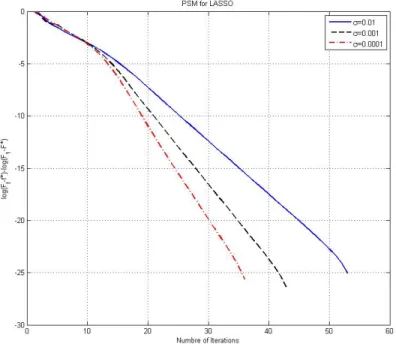
and is defined as kyk∞= maxi|yi|. We measure the converging of the PSM algorithm by computing the following normalized error function.
error(r) = log
F(xr)−F(x∗)
F(x1)−F(x∗)
for every iteration r. Since our analysis guarantees a linear rate of convergence for the PSM algorithm when applied to the LASSO problem, we expect this function to be linearly decreasing.
Figure 3.1 shows the error functionerror(r) versus the iteration numberr for three different values of noise variance, σ = 10−4,10−3,10−2. As the figure shows, the con-vergence of the PSM algorithm is linear for the LASSO problem.
Chapter 4
Block Coordinate Descent
Method
The block coordinate descent method (BCD) has a long history in optimization and numerical analysis.
In this chapter we will show that, the BCD algorithm is also a special case of the APS framework. The convergence rate of APS class of algorithms was analyzed under a local error bound condition (see the previous chapter). Therefore, our result implies the linear convergence rate of Block Coordinate Descent Method (BCD) for (1.1) for the LASSO or group LASSO type of problems when f1(x) =PJ∈J wJkxJk2
orf1(x) =PJ∈J wJkxJk2+λkxk1. The BCD algorithm is one of the main algorithms
used to solve large scale optimization problems due to the simplicity of its updates (especially for the LASSO or group LASSO type of problems in which each step of BCD is equivalent to a shrinkage operator [22]). This linear convergence result provides theoretical proof for effectiveness of BCD in handling such problems. In the sequel, we formally define the BCD method and introduce the main assumptions required for our convergence analysis of this algorithm.
Let x ∈ Rn have the block form of x = (x
1,x2, ...,xK)0, where xk ∈ Rik and
PK
k=1ik = n. Consider the minimization problem (1.1), in which f1 is separable over
the blocks. In other words it can be written as
f1(x) =d1(x1) +· · ·+dK(xK), (4.1) wheredk, k= 1,· · · , K are all convex (but not necessarily smooth) functions. Further-more, Xis a closed convex set in Rnwhich is also separable over the blocks, i.e. it can
be written as the following Cartesian product
X=X1×X2×...×XK, (4.2) where Xk is a closed convex subset of Rik. Note that the LASSO problem (1.3), group
LASSO problem (1.5) and logestic group LASSO problem (1.6) admit the decomposition specified by (4.1) and (4.2).
Consider the BCD method whereby after the r-th iteration, r ≥ 0, we choose an index s ∈ {1,2, ..., K} and compute the new iterate xr+1 = (x1r+1,xr2+1, ...,xrK+1) as follows
xrs+1 = argminxs∈XsF(x
r
1,xr2, ...,xrs−1,xs,xrs+1, ...,xrK)
xrj+1 =xrj, j 6=s. (4.3)
where (xr1,xr2, ...,xrK) denotes the iterate atr-th iteration. The blocks are chosen cycli-cally or essentially cyclicycli-cally to be updated at every iteration. The essentially cyclic update ensures that there exists an integer N ≥K such that after this many iterations all the blocks are updated at least once.
It is known [27] that the BCD algorithm with cyclic update or essentially cyclic up-date converges to the optimal solution for the set of non-smooth optimization problems that the non-smooth part is separable as defined in (4.1).
To establish linear convergence of the BCD method, we need the assumption that the smooth part f2 is strongly convex in each block, in the sense that there exists a
scalar γ ≥0 such that, for any x= (x1,x2, ...,xK)∈X and any s∈ {1,2, ..., K},
for all feasible ∆xs∈Ris, where∇sf2denotes the vector of partial derivatives off2 with
respect to the s-th block. It is obvious that if the function f2 is block coordinate-wise
strongly convex, then the coordinate descent method satisfies the sufficient decrease condition (3.3) [cf. Proposition 3.4 in [14]].
For the applications described in chapter 1, the coordinate-wise strong convexity of
f2 imposes a mild condition on the linear operatorA. For example, in LASSO problem
(1.3), if each column of Ais non-zero and we consider each element in xto be a block, then the problem is coordinate-wise strongly convex. Furthermore, for the group LASSO problem,f2 is block coordinate-wise strongly convex if the columns ofA corresponding
to a block are linearly independent. A similar condition can be derived for the logestic group LASSO problem (1.6) to ensure block coordinate-wise strong convexity. The following proposition shows that the block coordinate descent method for theL1 norm
minimization problem and the Group LASSO minimization problem is an APS method. Proposition 3 Under the above assumptions in (4.1), (4.2)and (4.4), the block coor-dinate descent method with cyclic update can be written in the APS form with an error term ewhich satisfies (3.2).
Proof Let us define two different iteration counters. The outer iteration index s is a counter for the number of updating cycles of the BCD algorithm, and the inner iteration index k corresponds to the variable block being updated in a given cycle. Thus, at iteration r = sK +k (with 1 ≤ k ≤ K), the k-th variable block is updated in the
s-th cycle. Throughout the proof, the notation xr means the r-th iterate of the BCD algorithm, and xrk represents the k-th block ofr-th iterate.
For simplicity, let us assume that there are no constraints. This assumption is not restricting as one can always add the indicator functions of the constraining sets to the objective. Since the feasible set is assumed to have a special structure as in (4.2), the separability of the non-smooth objective component will still be preserved after this change.
The optimality condition at the r-th iteration for BCD method is,
for some g in∂dk(xrk) (Note that we assumedf1(x) =d1(x1) +· · ·+dK(xK)). Now in each fixed cycle s, definer0 =Ksand the error vectores= (es1,· · ·,esK), as follows
esk =xrk0+k−xrk0 +∇kf2(xr
0
)− ∇kf2(xr
0+k
), ∀ k= 1,· · · , K. (4.6) Then, it is obvious thatxr0+K generated by BCD can also be derived from the following update rule
x(s+1)K= proxf1(xsK− ∇f2(xsK) +es). (4.7)
Now we can show that kesk ≤κkx(s+1)K−xsKkfor someκ >0. Sincef
2has Lipschitz
continuous gradient, it follows that kes kk ≤ kx r0+k k −x r0 kk+k∇kf2(xr 0 )− ∇kf2(xr 0+k )k ≤ kxrk0+k−xrk0k+Lkxr0−xr0+kk ≤ (L+ 1)kxr0+k−xr0k ≤ (L+ 1)kxr0+K−xr0k = (L+ 1)kx(s+1)K−xsKk,
where the second step is due to the Lipschitz condition on ∇f2 and the last inequality
is due to the block coordinate-wise update in the algorithm. This further implies that kesk ≤K(L+ 1)kx(s+1)K−xsKk,
so that the condition (3.2) holds with κ=K(L+ 1).
Remark 1 Note that a similar proof can be done to show that BCD algorithm with essentially cyclic update lies within the APS framework, with an error term e which satisfies (3.2).
The following Proposition is a direct consequence of Corollary 1 and Proposition 3. Proposition 4 The BCD algorithm (with cyclic or essentially cyclic update) generates a sequence of iterates that converges R-linearly to a solution in X∗ for LASSO problem
(1.3), Group LASSO problem (1.5) and logistic Group LASSO problem (1.6), if the objective function is block coordinate-wise strongly convex.
4.1
Related Works
To our knowledge this is the first result which shows the linear convergence rate of the exact BCD algorithm for solving problem (1.1) without requiring the strong convexity of the objective function. Here we would like to survey past works relating to our results: Earliest studies on the convergence rate of the BCD algorithm required the smoothness of the objective function [15], [31], [14]. These works showed that when the objective function is smooth (but not necessarily strongly convex) the BCD algorithm with the Gauss-Seidel update rule converges linearly, provided that the local error bound condition is satisfied around the solution set. The (Block) Coordinate Gradient Descent (abbreviated as CGD) algorithm proposed in [30] is a relevant method to BCD which can solve non-smooth problem (1.1) under the assumptions (4.1)-(4.2). As shown in [30], this algorithm enjoys having linear rates of convergence when the local error bound condition holds. The BCD and CGD algorithms both exploit block coordinate-wise updates to solve the problem (1.1). However, unlike BCD which solves the exact subproblem in each iteration, CGD approximates the smooth component f2 by a strictly convex quadratic
function. Therefore, the analysis given in [30] does not prove the linear convergence rate property of the exact BCD algorithm.
The Block Successive Upper-bound Minimization (BSUM) approach, studied in [32], is a general inexact BCD method for minimizing a (possibly non-convex) objective F
over a decomposable feasible set X formed as in (4.2). BSUM updates the variable blocks by successively minimizing a sequence of approximations of F which are locally tight upper-bounds of this function. The convergence analysis in [32] shows the iterates generated by the BSUM algorithm converge to the set of stationary points when the function level sets are compact. However, it does not imply any convergence rate results for the BCD algorithm. From a different perspective, BSUM can be viewed as a BCD variant of the majorization-minimization (also called successive upper-bound minimiza-tion) method. The convergence analysis of the majorization-minimization algorithm is done in [33]. As shown in that work, this algorithm exhibits linear rates of convergence when the objective function satisfies the strong convexity assumption.
Another relevant line of work is done in [34], [35], [36], [37], [38] which study ran-domized versions of BCD for solving problem (1.1). In each iteration of the ranran-domized
algorithm, a block of variables is randomly picked according to some probability distri-bution; Then, a strictly convex objective approximation, constructed in a similar way as in [30], is minimized with respect to those variables. Since the approximation function is (block) separable across the variables, the updates can be implemented in a distributed fashion. When the assumptions (4.1)-(4.2) hold, the authors in [35] prove that the ran-domized algorithm exhibits a global linear convergence rate in probability when a, so called, generalized error bound condition holds for the problem. In contrast to their analysis, we consider the case where the variables are updated in a cyclic (or essentially cyclic) fashion by minimizing the exact objective function. Therefore, our convergence rate results provide deterministic gurantees when the local error bound condition holds. In [36], the randomized BCD is applied for solving problem (1.1) when the variables are coupled with linear constraints. The analysis given in [36], [37] and [38] prove the linear convergence rate of the randomized BCD algorithm under the restricting assumption of the objective function being strongly convex. Further related works on the distributed implementation of the randomized BCD algorithm can be found in [39], [40], [41].
Beside the extensive interest in the randomized version of the BCD algorithm, the iteration complexity of the deterministic version is also studied recently [42], [43]. For a unified iteration complexity analysis for a family of BCD-type algorithms with either Gauss-Seidel or randomized coordinate update rules, the readers can refer to [44].
4.2
Simulation Results
4.2.1 LASSO Problem
In this section, we use the coordinate descent algorithm to solve the LASSO problem (1.3). We assume a linear data model as
b=Ax+e, (4.8)
where A= [a1,a2,· · · ,an]∈Rm×n,x∈Rn and e∈Rm are generated randomly as in
section 3.4.
The algorithm works by cyclically updating the coordinates. Therefore, at iteration
problem xri = arg min xi 1 2kb− n X j=1, j6=i aixrj−1−aixik22+λ|xi|. (4.9) Let zri =b−P j=1, j6=iaix r−1
j . Then the optimal solution to (4.9) is given by
xri = soft 1 aTiai zri; λ aTi ai ,
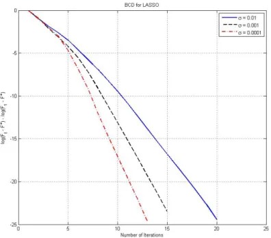
which is a very simple update rule. The algorithm will be terminated if the stopping criterion (3.15) is met. We evaluate the convergence of the coordinate descent algorithm by using the following relative error function
error(r) = log F(xr)−F(x∗) F(x1)−F(x∗) (4.10) for iterations r = kn. Since our analysis guarantees a linear rate of convergence for the BCD algorithm when applied to the LASSO problem, we expect this function to linearly decrease when the number of iterations is sufficiently large. Figure 4.1 shows the error function versus the cycle numberkfor three different values of noise variance,
σ = 10−2,10−3,10−4. As can be seen in this figure, the error function is indeed linearly decreasing with the cycle number.
Figure 4.1: Convergence of CD for the LASSO problem 4.2.2 Group LASSO Problem
We now illustrate the use of the block coordinate descent algorithm with group sparse regularization functions.Whenx∗ has a predefined block structure, it can be estimated by solving the group LASSO problem
min x∈Rn 1 2kAx−bk 2 2+λ X J∈J kxJk2
whereb=Ax∗+e. Our simulations in this subsection uses synthetic data and is mainly designed to show the efficiency of BCD in solving the group LASSO subproblem.
The matrixA∈Rm×n has dimensionsm= 210 and n= 212 and is filled with i.i.d.
standard Gaussian entries. The true vector x∗ has n = 212 components, divided into
n0 = 64 groups of length l= 64. To generate x∗, we randomly choose 8 groups and fill them with zero-mean Gaussian random samples of unit variance, while all other groups are filled with zero (this construction was taken from section 4 of [10]). The error vector is white Gaussian noise with varianceσ. Finally the value ofλwas set toλ= 0.1kATyk.
Figure 4.2 shows the original signal as well as the perfectly reconstructed one.
Figure 4.2: Comparison of the original and the BCD reconstructed vectors for group LASSO Like in the case of the LASSO problem, the BCD method has simple updates when applied to group LASSO problem. In particular, in iteration r=kn0+i, thei-th block of xis updated according to the following formulation
xri = arg min xi∈Rl 1 2kb− X J∈J,J6=i AJxrJ−1−Aixik22+λkxik2. (4.11) Definingzri =b−P
J∈J,J6=iAJxrJ−1, the first order optimality condition of the problem (4.11) implies that
ATi (Aixri −zir) +λg= 0, for someg ∈∂kxrik2.
If kAT
i Aizirk2 ≤ λ, then the optimal solution is zero, i.e. xri = 0. Otherwise, the optimal solution is given by
xri = ATi Ai+λ δIl
−1 ATi zir,
where Il is an identity matrix of size l (remember that l is the size of each block of variables) and δ is a positive constant which is also equal to δ = 1/kxr
ik2 and can be
found using the bisection method.
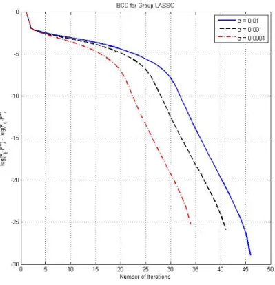
Figure 4.3 shows the relative error, defined in (4.10), as a function of the cycle number for three different values of the noise variance. The error function has a linear decrease after a few number of iterations, which implies the linear convergence rate of the BCD method in the case of the group LASSO problem.
Figure 4.3: Convergence of BCD for the Group LASSO problem 4.2.3 Support Vector Machine Classification
Support vector machines (SVM) are very effective tools for the purpose of classification learning. The task of learning is typically cast as a constrained quadratic problem. Formally, given a training set S ={(xi, yi)}ni=1, where xi ∈Rm and yi ∈ {−1,+1}, we
would like to find the minimizer of the following problem min α∈Rn 1 2α TKα−eTα (4.12) subject to 0≤αi≤C,∀i,
where K ∈ Rn×n is called the Kernel matrix and e ∈ Rn is the vector of all ones.
In the case of linear SVM, the entries of the kernel matrix are given by the equation
Ki,j =yixTi xjyj. In many large-scale classification problems, the kernel matrix is dense and ill-conditioned making the problem (4.12) challenging to solve.
The problem (4.12) has the form of the formulation (1.1) withf2(α) = 12αTKα−
eTαandf1(α) =ιC(α), whereιC(α) is the indicator function of the feasible set defined by the box constraints. Moreover, this problem satisfies the local error bound condition (see Theorem 1 in Chapter 2). Since the feasible set can be expressed as a Cartesian product of closed convex sets as in (4.2) and the objective function is strictly convex in each variable αi, the BCD algorithm can be applied for solving this problem. As illustrated in [45], the coordinate descent method can update the variables via very simple updates. Assume that the algorithm updates the coordinates in a cyclic manner, i.e. it cycles through {1},{2},· · ·,{n}. Then at iterationr =kn+i,k ∈Z, the i-th
coordinate αi must be updated by solving the following problem
αri = arg min αi∈R
f2(αr1, αr2,· · · , αri−1, αi, αri+1−1,· · · , αrn−1) (4.13) subject to 0≤αi ≤C.
The first-order optimality condition of this problem implies that the optimal solution is αri =αir−1 (i.e. αri−1 does not need to be updated) if and only if ∇P
i f2(αk
−1) = 0,
where ∇Pf
2(α) is the projected gradient vector defined as
∇Pi f2(α) = ∇if2(α) if 0< αi< C, min(0,∇if2(α)) ifαi = 0, max(0,∇if2(α)) ifαi =C.
αri−1. Otherwise, we must find the optimal solution of 4.13 which is given by αri = min max αri−1−∇if2(α r) Ki,i ,0 , C
where ∇if2(α) = (Kα)i−1 andKi,i =xTi xi.
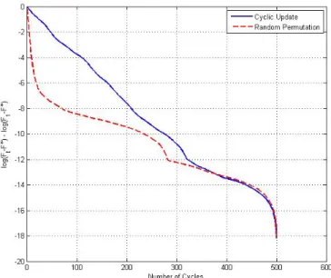
Here, we would like to illustrate the linear convergence of the coordinate descent algorithm for solving the SVM problem. In this experiment, we also use the coordinate descent algorithm with random coordinate selection and compare its performance with the one which uses cyclic coordinate selection. At the beginning of each cycle of the randomized algorithm, a permutation of {1,· · · , n} is randomly chosen and then the variables are updated in the order specified by this permutation. Past results [45] show that solving sub-problems in a random order may give faster convergence.
Our experiments in this subsection are based on a real-world dataset which is a subset of the Reuters Corpus dataset (RCV11 Dataset [46]). RCV1 is a benchmark dataset for text classification. The RCV1 subset that was used in this experiment contains 9625 doc-uments with 29992 distinct words, including categories“C15”,“ECAT”,“GCAT”, and “MCAT”, each with 2,022, 2,064, 2,901, and 2,638 documents respectively. In order to do binary classification, the C15 and ECAT categories were labeled as positive and GCAT and MCAT were labeled as negative [47]. In our experiments, we set C= 10.
Figure 4.4 shows the training accuracy of the BCD method which is defined as 1 n n X i=1 1{yi = ˆyi} where ˆyi = sign wTxi
is the estimated class for the i-th training example and is obtained by using the linear classifier w =Pn
j=1αjyjxj. As the figure shows, after a
few iterations, the algorithm correctly classifies almost all of the training examples. The figure also shows that the random update rule requires very few cycles to provide the correct classification of the training data.
1
The RCV1 dataset is available publicly at http://www.csie.ntu.edu.tw/cjlin/libsvmtools/
Figure 4.4: Training Accuracy of BCD
Figure 4.5 shows the relative error defined in (4.10) for the BCD algorithm, with both cyclic and random update rules. As the figure shows, the cyclic BCD has a linear rate of convergence. The randomized algorithm shows an even faster convergence behavior.
Chapter 5
Conclusion
In this thesis we have introduced the class of approximate proximal splitting methods and established its linear convergence under some conditions (sufficient decrease and local error bound). This general result implies the linear convergence of the BCD algorithm for a class of non-smooth convex problems. As a future work, it will be interesting to generalize the proofs of linear convergence for the APS algorithms to the problems with nuclear norm regularization [48], [49].
References
[1] R. Tibshirani. Regression shrinkage and selection via lasso. Journal of the Royal Statistical Society: Series B, 58:267–288, 1996.
[2] M. Yuan and Y. Lin. Model selection and estimation in regression with grouped variables.
Journal of the Royal Statistical Society: Series B, 68:49–67, 2006.
[3] L. Meier, S. Van De Geer, and P. Buhlmann. The group lasso for logistic regression.Journal of Royal Statistical Society: Series B, 70(1):53–71, 2008.
[4] F. Bach. Consistency of the group lasso and multiple kernel learning. The Journal of Machine Learning Research, 9:1179–1225, 2008.
[5] S. Ma, X. Song, and J. Huang. Supervised group lasso with applications to microarray data analysis. BMC bioinformatics, 8(1):60, 2007.
[6] D. Kim, S. Sra, and I. Dhillon. A scalable trust-region algorithm with applications to mixed-norm regression. International Conference of Machine Learning (ICML), 1, 2010. [7] J. Liu, S. Ji, and J. Ye. Slep: Sparse learning with efficient projections. Arizona State
University, 2009.
[8] V. Roth and B. Fischer. The group-lasso for generalized linear models: Uniqueness of solutions and efficient algorithms. In Proceedings of the 25th International Conference on Machine Learning, ACM, pages 848–855, 2008.
[9] E. Van Der Berg, M. Schmidt, M. Friedlander, and K. Murphy. Group sparsity via linear-time projection. Technical Report TR-2008-09, Department of Computer Science, Univer-sity of British Columbia, 2008.
[10] S. Wright, R. Nowak, and M. Figueiredo. Sparse reconstruction by separable approximation.
IEEE Transaction on Signal Processing, 57:2479–2493, 2009.
[11] J. B. Rosen. The gradient projection method for non-linear programming, part I linear constraints.Journal of Society of Industrial and Applied Mathematics, 8(1):181–217, March 1960.
[12] J. B. Rosen. The gradient projection method for linear programming, part II non-linear constraints. Journal of Society of Industrial and Applied Mathematics, 9(4):514–532, December 1961.
[13] P. Tseng. Approximation accuracy, gradient methods, and error bound for structured convex optimization. Mathematical Programming, (Technical Report), 2009.
[14] Z.-Q. Luo and P. Tseng. Error bounds and convergence analysis of feasible descent methods: A general approach. Annals of Operations Research, 46:157–178, 1993.
[15] Z.-Q. Luo and P. Tseng. On the linear convergence of descent methods for convex essentially smooth minimization. SIAM Journal on Control and Optimization, 3(2):408–425, March 1992.
[16] Z.-Q. Luo and P. Tseng. Analysis of an approximate gradient projection method with ap-plications to the back-propagation algorithm. Optimization Methods and Software, Special Issue Neural Networks via Mathematical Programming, 4:85–101, 1994.
[17] O. L. Mangasarian. Convergence of iterates of an inexact matrix splitting algorithm for the symmetric monotone linear complementarity problem.SIAM Journal on Optimization, 1(1):114–122, February 1991.
[18] W. Li. Remarks on the convergence of the matrix splitting algorithm for the symmetric linear complementarity problem. SIAM Journal on Optimization, 3(1):155–163, February 1993.
[19] J.-S. Pang. On the convergence of the basic iterative method for the implicit complemen-tarity problem. Journal of Optimization Theory and Applications, 37:149–162, 1982. [20] G. M. Korpelevich. The extra-gradient method for finding saddle points and other problems.
Ekon. i Mat Metody, Trasnlated to English as Matecon, 12:747–756, 1976.
[21] P. L. Combettes and V. R. Wajs. Signal recovery by proximal forward-backward splitting.
Multiscale Modeling and Simulation, 4:1168–1200, 2005.
[22] H. Zhang, J. Jiang, and Z.-Q. Luo. On the linear convergence of proximal splitting method for a class of nonsmooth convex minimization problems. Journal of Operations Research Society of China, 1:163–186, June 2013.
[23] R. S. Dembo and U. Tulowizki. Local convergence analysis for successive inexact quadratic programming methods. Working Paper, School of Organization and Management, Yale University, New Haven, 1984.
[24] J.-S. Pang. Inexact newton methods for nonlinear complementarity problem. Math. Prog., (36):54–71, 1986.
[25] J.-S. Pang. A posteriori error bounds for the linearly-constrained variational inequality problem. Math. Oper. Res., (12):474–484, 1987.
[26] Z.-Q. Luo and P. Tseng. Error bound and convergence analysis of matrix splitting algorithm for the affine variational inequality problem. SIAM Journal on Optimization, 2(1):43–54, February 1992.
[27] P. Tseng. Convergence of block coordinate method for non-differentiable minimization.
Journal of Optimization Theory and Appplications, 109(3):475–494, June 2001.
[28] A. Agarwal, S.N. Negahban, and M.J. Wainwright. Fast global convergence of gradient methods for high-dimensional statistical recovery. Annals of Statistics, 40(5):2452–2482, 2012.
[29] M. Schmidt, N.L. Roux, and F. Bach. Convergence rates of inexact proximal-gradient methods for convex optimization. Arxiv preprint arXiv:1109.2415, 2011.
[30] P. Tseng and S. Yun. A coordinate gradient descent method for nonsmooth separable minimization. Mathematical Programming, 117(1-2):387–423, 2009.
[31] Z.-Q. Luo and P. Tseng. On the linear convergence of descent methods for convex essentially smooth minimization. SIAM Journal on Control & Optimization, (30), March 1992. [32] M. Razaviyayn, M. Hong, and Z.-Q. Luo. A unified convergence analysis of block
succes-sive minimization methods for nonsmooth optimization. SIAM Journal on Optimization, 23(2):1126–1153, 2013.
[33] J. Mairal. Incremental majorization-minimization optimization with application to large-scale machine learning. arXiv preprint arXiv:1402.4419, 2014.
[34] Z. Lu and L. Xiao. On the complexity analysis of randomized block-coordinate descent methods. arXiv preprint arXiv:1305.4723, 2013.
[35] I. Necoara and D. Clipici. Distributed random coordinate descent method for composite minimization. arXiv preprint arXiv:1312.5302, 2013.
[36] I. Necoara and A. Patrascu. A random coordinate descent algorithm for optimization problems with composite objective function and linear coupled constraints. Computational Optimization and Applications, pages 1–31, 2013.
[37] Y. Nesterov. Efficiency of coordinate descent methods on huge-scale optimization problems.
SIAM Journal on Optimization, 22(2):341–362, 2012.
[38] P. Richt´arik and M. Tak´aˇc. Iteration complexity of randomized block-coordinate descent methods for minimizing a composite function. Mathematical Programming, pages 1–38, 2012.
[39] J. K. Bradley, A. Kyrola, D. Bickson, and C. Guestrin. Parallel coordinate descent for l1-regularized loss minimization. arXiv preprint arXiv:1105.5379, 2011.
[40] I. Necoara. Random coordinate descent algorithms for multi-agent convex optimization over networks. IEEE Transactions on Automatic Control, 58:2001–2012, 2013.
[41] P. Richt´arik and M. Tak´aˇc. Parallel coordinate descent methods for big data optimization.
arXiv preprint arXiv:1212.0873, 2012.
[42] A. Saha and A. Tewari. On the nonasymptotic convergence of cyclic coordinate descent methods. SIAM Journal on Optimization, 23(1):576–601, 2013.
[43] A. Beck and L. Tetruashvili. On the convergence of block coordinate descent type methods.
SIAM Journal on Optimization, 23(4):2037–2060, 2013.
[44] M. Hong, X. Wang, M. Razaviyayn, and Z.-Q. Luo. Iteration complexity analysis of block coordinate descent methods. arXiv preprint arXiv:1310.6957, 2013.
[45] C.-J. Hsieh, K.-W. Chang, C.-J. Lin, S. Keerthi, and S. Sundararajan. A dual coordi-nate descent method for large-scale linear svm. In Proceedings of the 25th international conference on Machine learning, pages 408–415. ACM, 2008.
[46] D. Lewis, Y. Yang, T. Rose, and F. Li. Rcv1: A new benchmark collection for text categorization research. The Journal of Machine Learning Research, 5:361–397, 2004. [47] S. Paul, C. Boutsidis, M. Magdon-Ismail, and P. Drineas. Random projections for linear
support vector machines. arXiv preprint arXiv:1211.6085, 2012.
[48] J.-F. Cai, E. J. Candes, and Z. Shen. A singular value thresholding algorithm for matrix completion. SIAM Journal on Optimization, pages 1956–1982, January 2010.
[49] K.-C. Toh and S. Yun. An accelerated proximal gradient algorithm for nuclear norm regu-larized least squares problems. Pacific Journal of Optimization, 6:615–640, 2009.
Appendix A
Proof of Lemma 3
We defineh(α) =k∇f˜ (x, α)k for anyα >0. Hence, the first part of the lemma is to show that
αh(α) is increasing withα.
From the definition of the proximity operator (2.4) and the proximal gradient (2.8), we have
αh(α) = x−arg min y∈X αf1(y) + 1 2||y−(x−α∇f2(x))|| 2 .
By the change of variablez,y−x, we have
αh(α) = arg min z∈X0 αf1(x+z) + 1 2kz+α∇f2(x)k 2 = arg min z∈X0 αf1(x+z) + 1 2kzk 2+αzT∇f 2(x) , (A.1)
where X0 ={z|z =y−xfor somey∈X}. Then, we have
αh(α) = arg min z∈X0 αg(z) +1 2kzk 2 , (A.2)
where g(z) = f1(x+z) +zT∇f2(x) is a (non-smooth) convex function. Our goal now is to show that if 0< α1< α2, then
α1h(α1) =kz∗(α1)k ≤ kz∗(α2)k=α2h(α2)
where z∗(α) denotes the optimal solution of
min z∈X0 αg(z) +1 2kzk 2 . (A.3) 44
The optimality ofz∗(α1) implies that g(z∗(α1)) + 1 2α1 kz∗(α1)k2≤g(z) + 1 2α1 kzk2, ∀z∈X0
In particular, whenz is set toz∗(α2), we have
g(z∗(α1)) + 1 2α1 kz∗(α1)k2≤g(z∗(α2)) + 1 2α1 kz∗(α2)k2. (A.4) Similarly, the optimality of z∗(α2) implies that
g(z∗(α2)) + 1 2α2 kz∗(α2)k2≤g(z∗(α1)) + 1 2α2 kz∗(α1)k2. (A.5) Adding up the last two equations yields that
α2−α1 2α1α2 kz∗(α1)k ≤ α2−α1 2α1α2 kz∗(α2)k.
Since 0 < α1 < α2, the above inequality implies that kz∗(α1)k ≤ kz∗(α2)k. Note that the convexity of f1 (or equivalentlyg) was not used in this part.
Next we prove the second part of the lemma which states thath(α) is monotonically decreasing withα. Introducing the new variableu,α1z, the equation (A.2) can be rewritten as
h(α) = arg min u∈X00 αg(αu) +1 2α 2kuk2 or equivalently, h(α) = arg min u∈X00 1 αg(αu) + 1 2kuk 2 (A.6) where X00={u|u= α1(y−x), for somey∈X}. We defineu∗(α) as the optimal solution of
h(α) = min u∈X00 1 αg(αu) + 1 2kuk 2 . (A.7)
It suffices to show that
h(α1) =ku∗(α1)k ≥ ku∗(α2)k=h(α2),
for 0< α1< α2. The first order optimality condition of (A.7) atu∗(α) implies