By
Magnus Erik Hvass Pedersen
1Hvass Laboratories Report HL-1401
First edition May 17, 2014
This revision August 3, 2014
2Please ensure you have downloaded the latest revision of this paper from the internet: www.hvass-labs.org/people/magnus/publications/pedersen2014portfolio-optimization.pdf
Source code and data files are also available from the internet:
www.hvass-labs.org/people/magnus/publications/pedersen2014portfolio-optimization.zip Microsoft Excel spreadsheet with basic Kelly portfolio optimization is also available: www.hvass-labs.org/people/magnus/publications/pedersen2014portfolio-optimization.xlsx
Abstract
This paper uses Monte Carlo simulation of a simple equity growth model with resampling of historical financial data to estimate the probability distributions of the future equity, earnings and payouts of companies. The simulated equity is then used with the historical P/Book distribution to estimate the probability distributions of the future stock prices. This is done for Coca-Cola, Wal-Mart, McDonald’s and the S&P 500 stock-market index. The return distributions are then used to construct optimal portfolios using the “Markowitz” (mean-variance) and “Kelly” (geometric mean) methods. It is shown that variance is an incorrect measure of investment risk so that mean-variance optimal portfolios do not minimize risk as commonly believed. This criticism holds for return distributions in general. Kelly portfolios are correctly optimized for investment risk and long-term gains, but the portfolios are often concentrated in few assets and are therefore sensitive to estimation errors in the return distributions.
1
If you find any parts difficult to understand, or if you encounter any errors, whether logical, mathematical, spelling, grammatical or otherwise, please mark the document and e-mail it to: Magnus (at) Hvass-Labs (dot) Org
2
2
Nomenclature
IID Independent and identically distributed stochastic variables.
PDF Probability Density Function.
CDF Cumulative Distribution Function (Empirical).
Present value of future payouts, dividends and share-price. Annual growth rate used in valuation.
Discount rate used in valuation.
k Kilo, a factor
m Million, a factor
b Billion, a factor
Infinity.
Price-to-Book ratio:
Number of shares outstanding.
Price per share.
Market capitalization (also written market-cap):
Capital supplied by shareholders as well as retained earnings, not per-share.
Earnings available for payout to shareholders, not per-share.
Dividend payout, pre-tax, not per-share.
Amount used for share buyback.
Amount of share issuance.
Share buyback net of issuance:
Net payout from company:
Part of earnings retained in company:
Return on Assets:
Return on Equity:
means that equals
means that is greater than or equal to means that is approximately equal to Implication: means that implies
Bi-implication: means that and Multiplication: means that is multiplied by
Summation:
Multiplication:
Maximum of or . Similarly for
Logarithmic function with base (natural logarithm). Absolute value of (the sign of is removed).
Probability of the stochastic variable being equal to .
Expected (or mean) value of the stochastic variable .
Variance of the stochastic variable .
Standard deviation of the stochastic variable :
3
4
1.
Introduction
There are two problems in constructing investment portfolios. First is to estimate the probability distribution of possible returns on individual assets. Second is the combination of these assets into a portfolio that optimally balances conflicting performance criteria.
A popular form of portfolio optimization is due to Markowitz [1] [2] which maximizes the portfolio’s mean return and minimizes the variance. Such portfolios are called mean-variance optimal. The return variance is commonly believed to measure investment risk so the mean-variance optimal portfolios are thought to maximize the mean return while minimizing risk. However, the examples in sections 4.3 and 11.2 show that variance is actually useless as a risk measure for investing.
For the future distribution of asset returns, Markowitz [2] vaguely proposed to use statistical analysis of past asset returns adjusted with the probability beliefs of expert financial analysts. This paper takes another approach by using Monte Carlo simulation of the equity growth model by Pedersen [3] which samples historical financial data for a company and simulates its future equity, earnings, dividends, etc. and then multiplies the simulated equity with samples of the historical P/Book distribution to estimate future stock prices. This model is used on several companies as well as the S&P 500 stock-market index.
The Monte Carlo simulated stock returns are also used to construct so-called Kelly optimal portfolios [4], which work as intended provided we know the true probability distributions of future asset returns. But Kelly portfolios heavily weigh the assets with the best return distributions, so if the distributions are incorrect then the Kelly portfolios may severely overweigh the wrong assets.
The paper also studies the complex historical relations between financial ratios such as P/Book and P/E for the companies and S&P 500 index, and also compares them to the yield on USA government bonds.
1.1.
Paper Overview
The paper is structured as follows:
Section 2 describes the financial valuation formulas and the equity growth model.
Section 3 describes algorithms for Monte Carlo simulation.
Section 4 describes mean-variance portfolio optimization.
Section 5 describes Kelly portfolio optimization.
Section 6 briefly studies USA government bond yields.
Section 7 studies the S&P 500 stock-market index.
Sections 8, 9 and 10 study the companies Wal-Mart, Coca-Cola and McDonald’s.
Section 11 studies the mean-variance and Kelly optimal portfolios of these companies.
5
1.2.
Source Code & Data
The experiments in this paper have been implemented in the statistical programming language R which is freely available from the internet. The source-code and data-files are available at:
www.hvass-labs.org/people/magnus/publications/pedersen2014portfolio-optimization.zip
Time Usage
Executing this implementation on a consumer-level computer from the year 2011 typically requires only seconds or minutes for an experiment consisting of a thousand Monte Carlo simulations. Implementing a parallelized version or using another programming language might significantly decrease the time usage.
6
7
2.
Present Value
The present value of the dividend for future year is the amount that would have to be invested today with an annual rate of return , also called the discount rate, so as to compound into becoming after
years:
Eq. 2-1
In Williams’ theory of investment value [5], the value of a company to its eternal shareholders is defined as the present value of all future dividends. Let denote the present value of all future dividends prior to dividend tax and not per share. Assume the discount rate is constant forever. If the company has no excess cash, then the company will first have to generate earnings before paying dividends, so the present value is calculated starting from the next year . The present value is then:
Eq. 2-2
2.1.
Payout
Instead of paying dividends, companies may also buy back or issue shares. Share buyback net of issuance is:
Eq. 2-3
The sum of dividends and net share buybacks is called payout:
Eq. 2-4
The term payout is a misnomer for share buybacks net of issuance as argued by Pedersen [6] [7], because a share buyback merely reduces the number of shares outstanding which may have unexpected effects on the share-price and hence does not constitute an actual payout from the company to its remaining
shareholders. A more accurate term for the combination of dividends and share buybacks would therefore be desirable but the term payout will be used here and the reader should keep this distinction in mind. The part of the earnings being retained in the company is:
Eq. 2-5
This is equivalent to:
8 The ratio of earnings being retained in the company is:
Eq. 2-7
2.2.
Equity Growth Model
The company’s equity is the capital supplied directly by shareholders and the accumulation of retained earnings. Earnings are retained for the purpose of investing in new assets that can increase future earnings. Let be the equity at the end of year and let be the part of the earnings that are retained in year . The equity at the end of year is then:
Eq. 2-8
The accumulation of equity is:
Eq. 2-9
The Return on Equity (ROE) is defined as a year’s earnings divided by the equity at the end of the previous year. For year this is:
Eq. 2-10
This is equivalent to:
Eq. 2-11
Using this with the definition of payout from Eq. 2-6 gives:
9 The present value to eternal shareholders is then:
Eq. 2-13 2.2.1. Normalized Equity
The accumulation of equity in Eq. 2-9 can be normalized by setting so it is independent of the starting equity. This also normalizes the earnings calculated in Eq. 2-11 and the payouts calculated in Eq. 2-12, which allows for Monte Carlo simulation based solely on the probability distributions for and so the results can easily be used with different starting equity.
2.3.
Market Capitalization
Let be the number of shares outstanding and let be the market-price per share. The market-cap (or market capitalization, or market value) is the total price for all shares outstanding:
Eq. 2-14
The market-cap is frequently considered relative to the equity, which is also known as the price-to-book-value or P/Book ratio:
Eq. 2-15
This is equivalent to:
Eq. 2-16
Because the starting equity is normalized to one in these Monte Carlo simulations, see section 2.2.1, it is often convenient to express the formulas involving the market-cap in terms of the P/Book ratio instead.
2.4.
Share Issuance & Buyback
Share issuance and buyback changes the number of shares outstanding and hence affects the per-share numbers, such as earnings per share, equity per share and price per share.
The number of shares is normalized by setting . If the share buyback and issuance occurs when the shares are priced at then the number of shares changes according to the following formula, see Pedersen [6] [7] for details:
10
Where is defined in Eq. 2-3 and is calculated using Eq. 2-16 with Monte Carlo simulated equity and P/Book ratio:
Eq. 2-18
The number of shares is then used with the Monte Carlo simulated equity, earnings, etc. to find the per-share numbers. For example, the equity per per-share in year is calculated as:
Eq. 2-19
The price per share in year is calculated from Eq. 2-18 and Eq. 2-17:
Eq. 2-20
2.5.
Value Yield
The value yield is defined as the discount rate which makes the market-cap equal to the present value:3
Eq. 2-21
This may be easier to understand if the notation makes clear that the present value is a function of the discount rate by writing the present value as . The value yield is then the choice of discount rate that causes the present value to equal the market-cap:
Eq. 2-22
2.5.1. No Share Buyback & Issuance
First assume the company’s payout consists entirely of dividends so there are no share buybacks and issuances and the number of shares remains constant.
The value yield for an eternal shareholder must then satisfy the equation:
Eq. 2-23 3
The value yield is also called the Internal Rate of Return (IRR) but that may be confused with the concept of the Return on Equity (ROE) and is therefore not used here.
11
For a shareholder who owns the shares and receives dividends for years after which the shares are sold at a price of , the value yield must satisfy the equation:
Eq. 2-24
2.5.2. Share Buyback & Issuance
If the company makes share buybacks and/or issuances then the number of shares changes and the present value is calculated from the dividend per share instead of the total annual payout. For an eternal
shareholder, the value yield must satisfy:
Eq. 2-25
For a temporary shareholder who owns the shares and receives dividends for years after which the shares are sold at a price of , the value yield must satisfy the equation:
Eq. 2-26 2.5.3. Tax
Taxes are ignored here but could also be taken into account. Let be the dividend tax-rate and let be the capital gain tax-rate, both in year . Assuming there is a capital gain when the shares are sold, the value yield must satisfy the equation:
Eq. 2-27
2.5.4. Interpretation as Rate of Return
The value yield is the annualized rate of return on an investment over its life or holding period, given the current market price of that investment. This follows from the duality of the definition of the present value from section 2, in which the present value may be considered as the discounting of a future dividend using a discount rate , or equivalently the future dividend may be considered the result of exponential growth of the present value using as the growth rate. The choice of that makes the present value equal to the market-cap is called the value yield. This interpretation also extends to multiple future dividends that spread over a number of years or perhaps continuing for eternity, where the present value is merely the sum of all those future dividends discounted at the same rate.
12
Note that the value yield is not the rate of return on reinvestment of future dividends, which will depend on the market price of the financial security at the time of such future dividends.
2.6.
Terminal Value
The present value of the equity growth model in Eq. 2-13 is defined from an infinite number of iterations, but the Monte Carlo simulation must terminate after a finite number of iterations. Estimating the present value is therefore done by separating into which is the present value of the payout in the
years that have been Monte Carlo simulated, and which is an approximation to the remaining
value if the Monte Carlo simulation had been allowed to continue for an infinite number of iterations:
Eq. 2-28
2.6.1. Mean Terminal Value
The mean terminal value can be estimated from the mean payout in year and the mean growth-rate which is assumed to continue indefinitely. A lower bound for this mean terminal value is derived in [3]:
Eq. 2-29
For the equity growth model in section 2.2, the mean growth rate is:
Eq. 2-30
When the equity at the end of year is known, the mean payout can be calculated from Eq. 2-12:
Eq. 2-31
The number of Monte Carlo iterations must be chosen large enough so the distortion introduced by the terminal value approximation is negligible. The formula for finding this number is given in [3].
13
3.
Monte Carlo Simulation
Monte Carlo simulation is computer simulation of a stochastic model repeated numerous times so as to estimate the probability distribution of the outcome of the stochastic model. This is useful when the probability distribution is not possible to derive analytically, either because it is too complex or because the stochastic variables of the model are not from simple, well-behaved probability distributions. Monte Carlo simulation allows for arbitrary probability distributions so that very rare events can also be modelled.
3.1.
Equity Growth Model
A single Monte Carlo simulation of the equity growth model consists of these steps: 1. Load historical financial data.
2. Determine the required number of Monte Carlo iterations using a formula from [3]. We set .
3. Set for normalization purposes.
4. For to : Sample , and from historical
data. The sampling is synchronized between companies as described below. Then calculate from Eq. 2-11, from Eq. 2-12, from Eq. 2-8,
, and .
5. Calculate the mean terminal value using Eq. 2-29. For finite holding periods use the market-cap (or share-price) as terminal value instead.
6. Use a numerical optimization method to find the value yield in Eq. 2-22.
The probability distribution is found by repeating steps 3-6 and recording the resulting value yields.
3.2.
Market-Cap
The simulated equity can be multiplied with a sample of the historical P/Book distribution to calculate the market-cap, see Eq. 2-16. However, this ignores the strong correlation of successive P/Book ratios in the historical data and may significantly distort the market-cap estimates, especially in the near future.
3.3.
Per Share
Calculating per-share numbers for equity, earnings, etc. consists of four steps:
1. The equity, earnings, share buyback net of issuance, etc. are simulated as described in section 3.1. 2. The market-cap is simulated as described in section 3.2.
3. The results of steps 1 and 2 are used with Eq. 2-17 and Eq. 2-18 to calculate the number of shares after share buyback and issuance.
4. The equity, earnings, etc. from step 1 are divided by the number of shares from step 3 to find the per-share numbers.
3.4.
Synchronized Data Sampling
The Monte Carlo simulation is performed for several companies simultaneously. To model any statistical dependency that might be in the historical data, the data sampling is synchronized between the companies. For example, the first year in the Monte Carlo simulation might use financial data from year 1998, the second year in the simulation might use data from year 2005, the third year might use data from year 1994, etc. This sequence of years is then used for all companies when sampling their historical financial data in step 4 of the Monte Carlo algorithm in section 3.1.
14
Similarly, when historical P/Book ratios are sampled for calculating the market-cap and share-price, the P/Book ratios are sampled from the same date for all companies. This is again done in an effort to model any statistical dependencies in the historical data.
3.5.
Warning
This paper uses a simple financial model with resampling of historical financial data to simulate the future finances and share-prices of companies, whose probability distributions are then used to construct portfolios. This is a paradigm shift from merely using past share-prices when constructing portfolios. However, the financial model is basic and has several limitations which should be kept in mind when interpreting the results: The equity growth model may not be suitable for the companies considered here. Growth decline should be modelled because the companies may otherwise outgrow the combined size of all the companies in the S&P 500 index, which is unrealistic. The financial data may be insufficient and data for more years might be needed e.g. to include long-term cycles. Older financial data should perhaps be sampled less frequently than newer data. Calculating future share-prices from the simulated equity multiplied with a sample of historical P/Book is a crude pricing model as mentioned in section 3.2.
15
4.
Mean-Variance Portfolio Optimization
Mean-variance portfolio optimization is originally due to Markowitz [1] [2]. A good description which also covers more recent additions to the theory is given by Luenberger [8].
4.1.
Portfolio Mean and Variance
Let denote the rate of return for asset and let denote the asset’s weight in the portfolio. For so-called long-only portfolios the assets can only be bought by the investor so the weights must all be positive . For so-called long-and-short portfolios the assets can be bought or sold-short so the weights can be either positive or negative. In both cases the weights must sum to one:
Eq. 4-1
The rate of return for the portfolio is:
Eq. 4-2
If there is uncertainty about the rate of return of an asset then is a stochastic variable which means the portfolio’s rate of return is also a stochastic variable. The mean is an estimate of the rate of return that can be expected from the portfolio. From the properties of the mean it follows that the portfolio’s mean rate of return is defined directly from the asset mean rates of return:
Eq. 4-3
The actual return of the portfolio may be very different from its mean return. There are several ways of measuring the degree of this uncertainty by measuring the spread of possible returns around the mean portfolio return. A common measure of spread is the variance. From the properties of the variance it follows that the portfolio’s variance is defined from the asset weights and the covariance of asset returns:
Eq. 4-4
The covariance measures how much the asset returns change together. A positive covariance means that the two asset returns have a tendency to increase together and vice versa for a negative covariance. If the covariance is zero then there is no consistent tendency for the asset returns to increase or decrease together; but this does not mean that the asset returns are independent of each other, merely that their relationship cannot be measured by the covariance.
16
4.2.
Optimal Portfolios – The Efficient Frontier
The mean and standard deviation of the asset returns can be plotted as in Figure 74. All possible portfolios that can be obtained by altering the weights are contained in the so-called feasible set. The feasible set is bordered by the so-called efficient frontier (also called the Pareto front in optimization terminology) which minimizes the portfolio variance for every portfolio mean in the feasible set. The efficient frontier contains the portfolios that are optimal in the sense that no lower variance can be obtained for a mean return. If we know the mean asset returns and the covariance matrix, then the efficient frontier can be found using the methods in [8].
4.3.
Variance is Not Risk
Mean-variance portfolios are commonly believed to minimize risk for a given level of expected return, because variance is believed to measure risk. But this is an incorrect notion as proven with a short example. Let asset A be a stochastic variable with negative returns (4%), (5%) or (6%) and let asset B be a stochastic variable with positive returns 5%, 10% or 15%. The returns have equal probability of occurring and are dependent in the order they are listed so that if asset A has return (4%) then asset B has return 5%, etc. The asset returns are perfectly anti-correlated with coefficient -1.
The long-only, minimum-variance portfolio lies on the efficient frontier and is when the weight for asset A is 5/6 and the weight for asset B is 1/6. This gives a portfolio with mean (2.5%) and zero variance, that is, all possible returns of the portfolio are losses of exactly (2.5%). But an investor could instead have chosen a portfolio consisting entirely of asset B which would always give a positive return of either 5%, 10% or 15%. An investment entirely in asset B is clearly superior to an investment in the minimum-variance portfolio. The above example had an asset with negative returns which could be avoided by adding the constraint that returns must be positive; but the problem also exists for assets with partly negative returns or all positive returns. To see this, change asset A’s possible returns to 3%, 2% or 1%. Then the minimum variance portfolio still has asset A weight 5/6 and asset B weight 1/6 which gives a portfolio return of about 3.3% with zero variance. But asset B alone would give a higher return of either 5%, 10% or 15%. So although the minimum-variance portfolio has no return spread, it has a lower return with certainty.
The problem also exists for assets that have overlapping return distributions. Let asset A’s possible returns be 6%, 5% or 4%. Then the minimum variance portfolio still has asset A weight 5/6 and asset B weight 1/6 which always gives a portfolio return of about 5.8% with zero variance. But asset B alone would give a higher return of either 10% or 15% with probability 2/3 (or about 67%) and a slightly lower return of 5% with probability 1/3 (or about 33%).
The reason asset A is included in the efficient frontier and minimum-variance portfolio is that its return has a low (sample) standard deviation of 1% while asset B has a higher standard deviation of 5%. The two assets have negative correlation so combining them in a portfolio lowers the combined standard deviation. The mean-variance efficient frontier is optimized for low variance (and standard deviation) which gives a low spread of the possible returns from the portfolio. But the spread of possible returns is not a useful measure of risk because it does not consider the probability of loss and the probability of other assets having a higher return. So the mean-variance portfolio is not optimized for risk in the traditional sense of the word which is defined in a dictionary as “the chance of injury or loss”.
17
This is also demonstrated in section 11.2 with more complicated return distributions.
4.4.
Value Yield
The value yield is the annualized rate of return over several years or for eternity. The value yield can be used as the rate of return in mean-variance portfolio optimization without changing the framework. The above criticism still applies, namely that variance does not measure investment risk.
18
5.
Kelly Portfolio Optimization
Kelly [4] proposed a formula for determining how much of one’s capital to place on a bet given the probability of gain and loss. The idea is to maximize the mean logarithmic growth-rate so that a sequence of bets in the “long run” and on average will most likely outperform any other betting scheme, but in the “short run” the Kelly betting may significantly underperform other betting schemes. The good and bad properties of Kelly betting are summarized by MacLean et al. [9]. The Kelly criterion is used here for a portfolio of assets where the returns of each asset are Monte Carlo simulated as described above.
5.1.
One Asset
Consider first the case where a single asset is available for investment. Let denote the stochastic rate of return on the asset and let denote the fraction of the portfolio invested in the asset. The remainder of the portfolio is held in cash which earns zero return.
The Kelly value (or Kelly criterion) is a function defined as:
Eq. 5-1
The objective is to find the asset weight that maximizes this Kelly value. 5.1.1. Only Positive Returns
If all asset returns are positive then the Kelly value in Eq. 5-1 increases as the asset weight increases. So the Kelly value is unbounded and suggests that an infinite amount of one’s capital should be invested in the asset using an infinite amount of leverage. This is because the cost of leverage is not taken into account.
5.2.
Two Assets
Now consider the case where two assets are available for investment whose returns are stochastic variables denoted and . The portfolio is divided between these two assets. The portfolio’s rate of return is the weighted sum of the asset returns:
Eq. 5-2
The Kelly value of the portfolio is:
Eq. 5-3
The objective is again to find the weight that maximizes the Kelly value. 5.2.1. One Asset and Government Bond
If one of the assets is a government bond then Eq. 5-3 has the bond yield as one of the asset returns:
19
5.3.
Multiple Assets
Now consider a portfolio of multiple assets. Let denote the stochastic rate of return on asset and let denote the weight of that asset in the portfolio. The portfolio’s rate of return is:
Eq. 5-5
The Kelly value is:
Eq. 5-6
The objective is again to find the weights that maximize the Kelly value. 5.3.1. Multiple Assets and Government Bond
If the portfolio can also contain a government bond then the portfolio’s rate of return is:
Eq. 5-7
The Kelly value is:
Eq. 5-8
The objective is again to find the weights that maximize the Kelly value.
5.4.
Constraints on Asset Weights
If the portfolio is so-called long-only then the weights must all be non-negative. If short-selling is allowed then the weights can also be negative. If leverage (investing for borrowed money) is disallowed then the sum of the weights must equal one. If leverage is allowed then the sum of the weights can exceed one.
5.5.
Value Yield
Recall from section 2.5.4 that the value yield is the annualized rate of return of an investment for a given holding period or eternity. This means the value yield can be used as the asset return in the Kelly formulas above. As demonstrated in the case studies below, the probability distribution for the value yield depends on the holding period. For long holding periods the value yield is mostly affected by the dividend payouts which are typically more stable, and for short holding periods the value yield is mostly affected by the
20
selling share-price which is more volatile. When using the value yield distributions in portfolio optimization it is therefore assumed that the holding period matches that of the value yield distributions.
For example, if a portfolio is to be optimized for a 10-year holding period, then the value yield distributions for 10-year holding periods should be used. Furthermore, if the portfolio may contain government bonds then the current yield on bonds with 10-year maturity should be used. The government bond is assumed to have a fixed yield if held until maturity, but if it is sold prior to its maturity then the selling price may cause the annualized yield to differ significantly.
5.6.
Optimization Method
When the asset returns are Monte Carlo simulated, the probability distributions are discrete with equal probability of all outcomes. An analytical method for determining the portfolio weights that maximize the Kelly value does not seem to exist in the literature. The so-called L-BFGS-B method was tested for
numerically optimizing the Kelly value but it did not work. A heuristic optimizer is therefore used here. 5.6.1. Differential Evolution
Differential Evolution (DE) was proposed by Storn and Price [10] for optimization without the use of gradients. DE works by having a population of candidate solutions for the optimization problem, which are combined through several iterations in an effort to improve their performance on the optimization
problem. This process resembles evolution as it occurs in nature. DE is not guaranteed to converge to the optimal solution but has been found to work in practice for many difficult optimization problems.
When optimizing Kelly portfolios, the candidate solutions of DE are different choices of portfolio weights and the performance measure that is sought maximized is the Kelly value in Eq. 5-8.
Control Parameters
DE has several control parameters that affect its performance and ability to find the optimum. The parameters used here are from Pedersen [11]. It may be necessary to select other parameters if the number of assets is greatly increased.
Constraints
The DE implementation used here has a simple constraint handling system which has boundaries for the portfolio weights, e.g. the weights must be between zero and one to disallow short-selling and leverage. But the weights must also sum to one and this is enforced by dividing each weight with the sum of weights in case the sum is greater than one. This works for simple constraints on the portfolio weights but if more complicated constraints are needed then the constraint handling system must be extended.
5.7.
Example of Correct Risk Minimization
Recall from section 4.3 that mean-variance portfolio optimization did not minimize for investment risk. This was demonstrated with two assets. Asset B is a stochastic variable with positive returns 5%, 10% or 15%. Three cases for returns on asset A were considered. In the first case, asset A has negative returns (4%), (5%) or (6%). In the second case, asset A has positive returns 3%, 2% or 1%. In the third case, asset A has positive returns 6%, 5% and 4% which overlap with the returns of asset B. In all these cases the returns have equal probability of occurring and are dependent in the order they are listed. Mean-variance portfolio
minimum-21
variance portfolios even though it is clearly inferior to a full investment in asset B. Even in the first case where asset A always results in losses, it was still included in the supposedly “minimum-risk” portfolio. Now consider the same assets where the portfolio is instead optimized using the Kelly criterion. Figure 76 shows the curves of Kelly values calculated using Eq. 5-3 for the different return distributions and varying the weight of asset A between zero and one while letting the weight of asset B equal one minus the weight of asset A. The objective is to find the asset weights that maximize the Kelly value and in all three cases the maximum Kelly value is when the weight of asset A equals zero and the weight of asset B equals one. That is, the Kelly optimal portfolios consist entirely of asset B. These are the correct portfolio allocations.
5.8.
Example with Simulated Returns
Also shown in Figure 76 is the Kelly curve when asset A has returns 12%, 9% or 9% and asset B has returns 5%, 10% or 15%. Note that the two assets have identical mean returns of 10% but asset A has a lower (sample) standard deviation of 1.7% while asset B has 5%.
From the Kelly curve in Figure 76, the Kelly optimal portfolio is found to have asset A weight about 0.756 and asset B weight about 0.244. The portfolio returns are calculated using these weights and Eq. 5-2:
That is, the Kelly portfolio has a return of either 10.3%, 9.2% or 10.5% with mean 10% and (sample) standard deviation about 0.7%. The Kelly value for this portfolio is calculated using Eq. 5-3:
The Kelly value for a portfolio consisting entirely of asset A is:
The Kelly value for a portfolio consisting entirely of asset B is:
So the portfolio consisting of asset A with weight 0.756 and asset B with weight 0.244 has a Kelly value that is slightly higher than either asset alone.
5.8.1. Simulated Returns
Figure 77 shows cumulative returns that are simulated by drawing synchronized samples from the return distributions of asset A, asset B and the Kelly optimal portfolio. The plots show the cumulative return of the Kelly portfolio divided by the cumulative returns of assets A and B. The Kelly portfolio returns are similar to the returns of asset A so they often have a ratio close to one. But the Kelly portfolio returns are more dissimilar to the returns of asset B so their ratio is usually different from one. The Kelly portfolio often
22
grows exponentially more than asset B, but sometimes the Kelly portfolio decreases significantly relative to asset B for extended periods.
The Kelly portfolio is optimal in the sense that in the “long run” its average growth is superior to all other possible portfolios consisting of these two assets, but in the “short run” the Kelly portfolio can significantly underperform, as evidenced in Figure 77.
5.9.
Markowitz’ Opinion on the Kelly Criterion
In Chapter VI of [2] Markowitz discussed the geometric mean return which is essentially the Kelly value in Eq. 5-1, and concluded that: “The combination of expected return and variance which promises the greatest return in the long run is not necessarily the combination which best meets the investor’s needs. The investor may prefer to sacrifice long-run return for short-run stability.” But Markowitz does not seem to mention that this alleged “stability” of mean-variance portfolios in fact may cause inferior returns and even losses, as demonstrated in section 4.3.
23
24
6.
USA Government Bonds
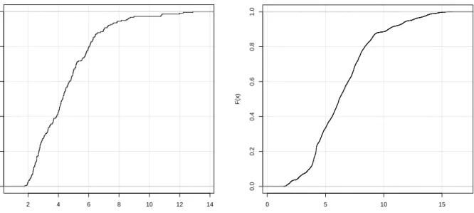
Figure 1 shows the historical yield on USA government bonds for the periods 1798-2012 (averaged annually) and 1962-2013 (averaged daily). During this period the bonds have had varying maturity period, terms and taxation. Table 1 shows the statistics with a mean yield about 5% and standard deviation about 2%. Figure 2 shows the histograms of these historical bond yields and Figure 3 shows the cumulative distribution functions. More statistics on USA government bonds are given by Pedersen [3].
7.
S&P 500
The Standard & Poor’s 500 stock market index (S&P 500) consists of 500 large companies traded on the stock markets in USA and operating in a wide variety of industries including energy and utility, financial services, health care, information technology, heavy industry, manufacturers of consumer products, etc. The S&P 500 index may be used as a proxy for the entire USA stock market as it covers about 75% of that market.4
7.1.
Financial Data
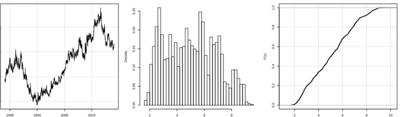
Table 2 shows financial ratios for the S&P 500 and statistics are shown in Table 3. Figure 4 shows the historical stock-price. The earnings yield is shown in Figure 5, the P/Book is shown in Figure 6, the P/E is shown in Figure 7 and statistics are shown in Table 4. Figure 8 compares the P/Book and P/E which shows a complex relation caused by the earnings having greater volatility than the book-value.
7.1.1. Comparison to USA Government Bonds
Figure 9 compares the yield on USA government bonds with 10-year maturity to the earnings yield and P/Book of the S&P 500, which shows complex relations. Figure 10 shows the difference between the earnings yield of the S&P 500 and the yield on USA government bonds which varies through time from negative (3.6%) to positive 5.9% with negative mean (0.4%), see Table 5. So if the S&P 500 had paid out all its earnings as dividends then the average rate of return would have been 0.4% (that is, percentage points) lower than the rate of return that could be obtained from investing in USA government bonds. This means the S&P 500 would either have to grow its earnings or the participants of the capital market viewed the S&P 500 as having lower risk than USA government bonds. This so-called equity risk premium between the S&P 500 and USA government bonds is studied in more detail by Pedersen [3]. The conclusion is that there is no consistent and predictable relation between the yield on USA government bonds and the rate of return on the S&P 500 stock-market index.
7.2.
Value Yield
The Monte Carlo simulation described in section 3 is performed 2,000 times using the financial ratios for the S&P 500 stock-market index in Table 2. The starting P/Book ratio for the S&P 500 is set to 2.6 calculated from the share-price of about USD 1,880 on April 24, 2014 divided by the last-known equity of USD 715.84 on December 31, 2013. The current P/Book of 2.6 is slightly below the historical average of 2.9, see Table 4.
4
S&P 500 Fact Sheet, retrieved April 11, 2013:
25
The Monte Carlo simulation provides estimates of future equity, earnings, dividends, etc. but only the value yield is used here. Recall that the value yield is the annualized rate of return an investor would get from making an investment and holding it for a number of years, see section 2.5.4.
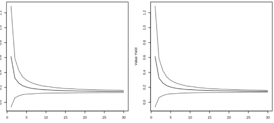
Figure 11 shows the mean and standard deviation for the value yield for holding periods up to 30 years. Note that the standard deviation decreases as the holding period increases. This is because when the holding period is short, the value yield is greatly affected by the selling price which is more volatile. When the holding period is long, the value yield is dominated by the dividend payouts which are more stable. Figure 12 shows the value yield distribution for 10 year holding periods and Figure 13 shows them for eternal holding periods. The value yield distributions with and without share buyback simulation are shown and although the difference is small it is not zero. Unless otherwise noted in the following we will use the value yield with share buyback simulation.
8.
Wal-Mart
The company Wal-Mart is an international retailer and was founded in 1962 in USA.
8.1.
Financial Data
Table 6 shows financial data for Wal-Mart. Financial ratios are shown in Table 7 and statistics are shown in Table 8. Note the low standard deviation of all these ratios except the ones regarding the allocation of earnings between dividends, share buyback and retaining.
Figure 14 shows the historical share-price. The earnings yield is shown in Figure 15, the P/Book is shown in Figure 16, the P/E is shown in Figure 17 and statistics are shown in Table 9. Figure 18 compares the P/Book and P/E which shows an almost linear relation caused by the stability of ROE so the earnings were closely related to the book-value (equity) and hence P/E is closely related to P/Book, see Table 8.
8.1.1. Comparison to USA Government Bonds
Figure 19 compares the yield on USA government bonds to the earnings yield and P/Book of Wal-Mart which shows complex relations that are somewhat correlated; the earnings yield has negative correlation coefficient (0.61) and the P/Book has positive correlation coefficient 0.44.
Figure 20 shows the difference between the earnings yield of Wal-Mart and the yield on USA government bonds. The statistics are shown in Table 11 and range between (4.9%) and 7.5% with mean 0.5%.
There is no clear and simple relation between the pricing of Wal-Mart shares and USA government bonds. 8.1.2. Comparison to S&P 500
Figure 21 compares the earnings yield, P/Book and P/E for Wal-Mart and the S&P 500 index. The relations are complex but the P/Book is highly correlated with coefficient 0.85, see Table 10.
Figure 22 shows the difference between the earnings yield of Wal-Mart and the S&P 500 index. The statistics are shown in Table 11. There is no consistent and predictable difference in earnings yield.
26
8.2.
Value Yield
The Monte Carlo simulation described in section 3 is performed 2,000 times using the financial ratios for Wal-Mart in Table 7. The starting P/Book ratio for Wal-Mart is set to 3.3 calculated from the market-cap of USD 253b on April 24, 2014 and divided by the last-known equity of USD 76b on January 31, 2014. The current P/Book of 3.3 is considerably less than the historical average of 4.7, see Table 9, and historically the P/Book has been greater than 3.3 about 70% of the time, see the P/Book CDF plot in Figure 16.
Figure 23 shows the mean and standard deviation for the value yield for holding periods up to 30 years. As noted previously, the standard deviation decreases as the holding period increases. Figure 24 shows the value yield distribution for 10 year holding periods and Figure 25 shows it for eternal holding periods. 8.2.1. Comparison to S&P 500
Figure 26 compares the value yields of Wal-Mart and the S&P 500 index for 10-year holding periods, which has positive correlation with coefficient 0.77, see Table 24. Figure 27 compares the value yields for eternal holding which has a positive but lower correlation with coefficient 0.34, see Table 25.
Figure 28 shows the value yield difference between Wal-Mart and the S&P 500 index for 10-year holding periods. The value yield differences are almost all positive and are about 7.5% on average. This means nearly all the value yields of Wal-Mart are greater than those of the S&P 500 index.
Figure 29 shows the distribution of value yield difference for eternal holding of Wal-Mart and the S&P 500 index. The value yield differences are almost all greater than 3.5% with mean about 5%. This means the value yield of Wal-Mart is at least 3.5% (percentage points) greater than that of the S&P 500 index, and on average the difference is 5% (percentage points).
The large differences in the value yields of these Monte Carlo simulations are partially caused by Wal-Mart’s dividend per share growing 12% per year on average while the dividend of the S&P 500 index only grows 6.3%. Furthermore, for 10-year holding periods the share-price significantly affects the value yield. The S&P 500 is currently trading slightly below its historical average P/Book while Wal-Mart is currently trading much below its historical average. As future share-prices are calculated here by sampling the historical P/Book distribution, the share-prices of Wal-Mart are likely to increase more than those of the S&P 500 index.
9.
Coca-Cola
The company Coca-Cola was incorporated in 1919 in USA but its origin is significantly older. The company produces beverages that are sold worldwide.
9.1.
Financial Data
Table 12 shows financial data for Coca-Cola. Financial ratios are shown in Table 13 and statistics are shown in Table 14. Note that all these ratios are considerably more volatile than those of Wal-Mart in Table 8. Figure 30 shows the historical share-price. The earnings yield is shown in Figure 31, the P/Book is shown in Figure 32, the P/E is shown in Figure 33 and statistics are shown in Table 15. Figure 34 compares the P/Book and P/E which shows a complex relation but with a high correlation coefficient of 0.78.
27 9.1.1. Comparison to USA Government Bonds
Figure 35 compares the yield on USA government bonds to the earnings yield and P/Book of Coca-Cola which shows complex relations but strong correlations; the earnings yield has negative correlation
coefficient (0.62) and the P/Book has positive correlation coefficient 0.72. This means that there has been a historical tendency for the P/Book to increase with the yield of USA government bonds although in a complex and unpredictable pattern.
Figure 36 shows the difference between the earnings yield of Coca-Cola and the yield on USA government bonds. The statistics are shown in Table 17 and range between (5.3%) and 5.5% with mean (0.4%). There is no consistent and predictable premium between the earnings yield of Coca-Cola and the yield on USA government bonds.
9.1.2. Comparison to S&P 500
Figure 37 compares the earnings yield, P/Book and P/E for Coca-Cola and the S&P 500 index. The relations are complex but the P/Book is somewhat correlated with coefficient 0.69, see Table 16.
Figure 38 shows the difference between the earnings yield of Coca-Cola and the S&P 500 index. The statistics are shown in Table 17. There is no consistent and predictable difference in earnings yield.
9.2.
Value Yield
The Monte Carlo simulation described in section 3 is performed 2,000 times using the financial ratios for Coca-Cola in Table 13. The starting P/Book ratio for Coca-Cola is set to 5.5 calculated from the market-cap of USD 179b on April 24, 2014 and divided by the last-known equity of USD 33b on March 28, 2014. The current P/Book of 5.5 is almost half of the historical average of 10.7, see Table 15, and historically the P/Book has been greater than 5.5 more than 75% of the time, see the P/Book CDF plot in Figure 32. Figure 39 shows the mean and standard deviation for the value yield for holding periods up to 30 years. As noted previously, the standard deviation decreases as the holding period increases. Figure 40 shows the value yield distribution for 10 year holding periods and Figure 41 shows it for eternal holding periods. 9.2.1. Comparison to S&P 500
Figure 42 compares the value yields of Coca-Cola and the S&P 500 index for 10-year holding periods, which has positive correlation with coefficient 0.65, see Table 24. Figure 43 compares the value yields for eternal holding which has a slightly positive correlation with coefficient 0.16, see Table 25.
Figure 44 shows the value yield difference between Coca-Cola and the S&P 500 index for 10-year holding periods. The value yield differences are almost all positive and are about 12.5% on average. This means nearly all the value yields of Coca-Cola are greater than those of the S&P 500 index.
Figure 45 shows the distribution of value yield difference for eternal holding of Coca-Cola and the S&P 500 index. The value yield differences are all greater than 5% with mean about 8%. This means the value yield of Coca-Cola is at least 5% (percentage points) greater than that of the S&P 500 index, and on average the difference is 8% (percentage points).
The large differences in the value yields of these Monte Carlo simulations are partially caused by Coca-Cola’s dividend per share growing 13% per year on average while the dividend of the S&P 500 index only
28
grows 6.3%. Furthermore, for 10-year holding periods the share-price significantly affects the value yield. The S&P 500 is currently trading slightly below its historical average P/Book while Coca-Cola is currently trading at half its historical average. As future share-prices are calculated by sampling the historical P/Book distribution, the share-prices of Coca-Cola are likely to increase more than those of the S&P 500 index.
10.
McDonald’s
The company McDonald’s was started by two brothers in USA in 1948 as a single restaurant selling fast-food at low prices. The company now sells its fast-fast-food worldwide.
10.1.
Financial Data
Table 18 shows financial data for McDonald’s. Financial ratios are shown in Table 19 and statistics are shown in Table 20. Note that all these ratios are volatile with high standard deviation except for the ratio of equity to assets.
Figure 46 shows the historical share-price. The earnings yield is shown in Figure 47, the P/Book is shown in Figure 48, the P/E is shown in Figure 49 and statistics are shown in Table 21. Figure 50 compares the P/Book and P/E which shows a complex relation with a somewhat low correlation coefficient of 0.25. 10.1.1.Comparison to USA Government Bonds
Figure 51 compares the yield on USA government bonds to the earnings yield and P/Book of McDonald’s which shows complex relations. The earnings yield has negative correlation coefficient (0.14) and the P/Book has negative correlation coefficient (0.53).
Figure 52 shows the difference between the earnings yield of McDonald’s and the yield on USA government bonds. The statistics are shown in Table 23 and range between (3.3%) and 4.9% with mean 0.4%. There is no consistent and predictable premium between the earnings yield of McDonald’s and the yield on USA government bonds.
10.1.2.Comparison to S&P 500
Figure 53 compares the earnings yield, P/Book and P/E for McDonald’s and the S&P 500 index. The relations are complex. The correlation coefficients are shown in Table 22 but are not useful in describing these complex relations.
Figure 54 shows the difference between the earnings yield of McDonald’s and the S&P 500 index. The statistics are shown in Table 23 and range between (1.7%) and 4.8% with mean 0.7%. There is no consistent and predictable difference in earnings yield.
10.2.
Value Yield
The Monte Carlo simulation described in section 3 is performed 2,000 times using the financial ratios for McDonald’s in Table 19. The starting P/Book ratio for McDonald’s is set to 6.2 calculated from the market-cap of USD 99b on April 24, 2014 and divided by the last-known equity of USD 16b on December 31, 2013. The current P/Book of 6.2 is much higher than the historical average of 4.0, see Table 21. Historically the P/Book has been lower than 6.2 more than 90% of the time, see the P/Book CDF plot in Figure 48.
29
Figure 55 shows the mean and standard deviation for the value yield for holding periods up to 30 years. As noted previously, the standard deviation decreases as the holding period increases.
10.2.1.Holding for 10 Years
Figure 56 shows the value yield distribution for 10 year holding periods. The value yield of McDonald’s for 10 year holding periods is negative with probability 0.13 (or 13%). The probability is 0.40 (or 40%) that the value yield of McDonald’s is less than the yield on USA government bonds with 10 year maturity, which was about 2.7% in late April 2014. On average the value yield of McDonald’s is 3.7%.
The high probability of loss is due to two things: (1) The current P/Book of McDonald’s is historically high and future share-prices are Monte Carlo simulated with mostly lower P/Book, and (2) the historical ROE is much lower than it has been in recent years so the simulated future earnings and the accumulation of equity is lower than it has been in recent years. The combined effect is a Monte Carlo simulated share-price that is often lower than it is today.
10.2.2.Holding for Eternity
Figure 57 shows the value yield distribution for eternal holding periods. When the effect of share buybacks is also Monte Carlo simulated then the value yield ranges between 6.5-9.5%. This is a large increase from the value yield for 10-year holding periods. The reason is that the volatile share-price has a small impact on the value yield when the holding period is eternity as there is no selling share-price. It is the dividends that determine the value yield. Furthermore, the decreasing share-price has a positive effect on the value yield when share buybacks are simulated because shares are bought back in the future at relatively lower prices. 10.2.3.Comparison to S&P 500
Figure 58 compares the value yields of McDonald’s and the S&P 500 index for 10-year holding periods, which has almost zero correlation, see Table 24. Figure 59 compares the value yields for eternal holding which has a positive correlation with coefficient 0.56, see Table 25.
Figure 60 shows the value yield difference between McDonald’s and the S&P 500 index for 10-year holding periods. The probability of McDonald’s value yield being less than that of the S&P 500 is 0.88 (or 88%). The value yield difference ranges between (14%) and 4% with mean (5.9%).
Figure 61 shows the distribution of value yield difference for eternal holding of McDonald’s and the S&P 500 index. The probability of McDonald’s value yield being less than that of the S&P 500 is 0.97 (or 97%). The value yield difference ranges between (2.1%) and 0.6% with mean (0.7%).
In both cases, nearly all the value yields of McDonald’s are less than those of the S&P 500. For the 10-year holding period this is partially caused by the decrease in McDonald’s simulated share-price as described above. For eternal holding the reason is that a high share-price is currently being paid for McDonald’s shares with a P/Book of 6.2 and the Monte Carlo simulated dividend per share grows about 6.4% per year on average. For the S&P 500 the dividend per share grows slightly less at about 6.3% per year on average, but shares of the S&P 500 are much lower priced at a P/Book of only 2.6. The initial simulated dividend yield is higher for the S&P 500 than for McDonald’s and because of the similar growth rates it is currently cheaper to purchase the dividend stream of the S&P 500 index than McDonald’s. The result is that S&P 500 has a higher value yield than McDonald’s.
30
11.
Portfolios
This section optimizes portfolios of the companies that were studied individually in the previous sections.
11.1.
Value Yield Comparison
The previous sections compared the value yields of the companies to that of the S&P 500 stock-market index. This section compares the value yields amongst companies. As described in section 3.4, the Monte Carlo simulations of companies are synchronized so that historical financial data is sampled from the same year amongst companies. This is done to account for statistical dependencies between the companies. 11.1.1.Wal-Mart & Coca-Cola
Figure 62 compares the value yields of Wal-Mart and Coca-Cola for 10-year holding periods which are positively correlated with coefficient 0.47, see Table 24. Figure 63 compares the value yields for eternal holding which are negatively correlated with coefficient (0.22), see Table 25.
Figure 64 shows the distribution of value yield differences between Wal-Mart and Coca-Cola for 10-year holding periods where there is a probability of 0.88 (or 88%) that Wal-Mart has a lower value yield than Coca-Cola, see Table 26. The value yield difference is on average about 5% (percentage points).
Figure 65 shows the value yield differences for eternal holding where there is a probability of 0.998 (or 99.8%) that Wal-Mart has a lower value yield than Coca-Cola, see Table 27. The value yield difference is on average about 3% (percentage points).
11.1.2.McDonald’s & Coca-Cola
Figure 66 compares the value yields of McDonald’s and Coca-Cola for 10-year holding periods which are slightly negatively correlated with coefficient (0.1), see Table 24. Figure 67 compares the value yields for eternal holding which are nearly uncorrelated with coefficient 0.03, see Table 25.
Figure 68 shows the distribution of value yield differences between McDonald’s and Coca-Cola for 10-year holding periods where there is a probability of almost 1 (or 100%) that McDonald’s has a lower value yield than Coca-Cola, see Table 26. The value yield difference is on average about 18% (percentage points). Figure 69 shows the value yield differences for eternal holding where there is a probability of 1 (or 100%) that McDonald’s has a lower value yield than Coca-Cola, see Table 27. The value yield difference is on average about 9% (percentage points).
11.1.3.McDonald’s & Wal-Mart
Figure 70 compares the value yields of McDonald’s and Wal-Mart for 10-year holding periods which are slightly negatively correlated with coefficient (0.11), see Table 24. Figure 71 compares the value yields for eternal holding which are slightly positively correlated with coefficient 0.19, see Table 25.
Figure 72 shows the distribution of value yield differences between McDonald’s and Wal-Mart for 10-year holding periods where there is a probability of almost 1 (or 100%) that McDonald’s has a lower value yield than Wal-Mart, see Table 26. The value yield difference is on average about 13% (percentage points).
31
Figure 73 shows the value yield differences for eternal holding where there is a probability of 1 (or 100%) that McDonald’s has a lower value yield than Wal-Mart, see Table 27. The value yield difference is on average almost 6% (percentage points).
11.1.4.Ordering
The value yields can be ordered as follows:
USA Government Bond < McDonald’s < S&P 500 < Wal-Mart < Coca-Cola
That is, the annualized rate of return on Coca-Cola is mostly greater than that of Wal-Mart, which is mostly greater than that of the S&P 500, which is mostly greater than that of McDonald’s, which is mostly greater than the yield on USA government bonds. However, the probabilities are not equal to one.
For 10-year holding periods there is a probability of 0.6 (or 60%) that the yield on USA government bonds is less than the value yield of McDonald’s; and there is a probability of 0.88 (or 88%) that the value yield of McDonald’s is less than that of the S&P 500; and there is a probability of 0.82 (or 82%) that the value yield of Wal-Mart is less than that of Coca-Cola; see Table 26 and Table 28. The probabilities can be written above the inequality signs in the ordering:
USA Government Bond <0.6 McDonald’s <0.88 S&P 500 <0.9965 Wal-Mart <0.82 Coca-Cola
Eq. 11-1
For eternal holding periods the relation is almost rigid as the probabilities are nearly one, see Table 27 and Table 28. The ordering is:
USA Government Bond <1 McDonald’s <0.97 S&P 500 <1 Wal-Mart <0.998 Coca-Cola
Eq. 11-2
11.1.5.Correlation
The value yields are somewhat correlated as shown in the scatter-plots and summarized in Table 24 and Table 25. However, the correlation coefficients change magnitude and in some cases also change signs for the different holding periods considered here. For example, for 10-year holding periods the value yields of Wal-Mart and Coca-Cola are positively correlated with coefficient 0.47 but for eternal holding the value yields are negatively correlated with coefficient (0.22).
11.2.
Mean-Variance Optimal Portfolios
This section optimizes portfolios with regard to the mean and variance as described in section 4, using the Monte Carlo simulated value yields described in the previous sections.
11.2.1.Holding for 10 Years
The mean-variance efficient portfolios for 10-year holding periods are shown in Figure 74 and the portfolio weights are shown in Table 29 and Table 30. Note that McDonald’s is contained in most of the efficient frontier for the long-only portfolios and is contained in the entire efficient frontier for the long-and-short portfolios. This is in spite of McDonald’s having a probability of nearly 1 (or 100%) of having a lower value yield than all the other assets available for the portfolio, see Table 26, and furthermore there is a
32
probability of 0.13 (or 13%) that McDonald’s value yield is less than zero and there is a probability of 0.4 (or 40%) that McDonald’s value yield is less than the return on USA government bonds, see Table 28.
11.2.2.Holding for Eternity
The mean-variance efficient frontiers for eternal holding periods are shown in Figure 75 and the portfolio weights are shown in Table 31 and Table 32. Note that McDonald’s is contained in half of the efficient long-only portfolios and almost all of the efficient long-and-short portfolios. This is in spite of McDonald’s having probability almost one of having a lower rate of return than the other assets, see Table 27.
11.2.3.Variance is Not Risk
The efficient portfolios contain McDonald’s even though it is almost certain to have a lower value yield than the other assets available for the portfolio. Furthermore, for 10-year holding periods there is a significant risk of McDonald’s having a lower value yield than the yield on USA government bonds – as well as a significant risk of McDonald’s value yield being negative.
The reason McDonald’s is included in the mean-variance efficient frontier is that McDonald’s value yields have a low variance (and standard deviation). The mean-variance efficient frontier is optimized for low variance which gives a low spread of the possible returns on the portfolio. But the spread of possible returns is not a useful measure of investment risk because it does not consider the probability of loss and the probability of other assets having a higher return. This criticism holds in general, see section 4.3.
11.3.
Kelly Optimal Portfolios
Recall the plots in Figure 74 showed the efficient frontier for mean-variance optimal portfolios, that is, the curved line where portfolios have maximum mean and minimum variance. Because there were two measures of performance – mean and variance – it was convenient to show the trade-off between these two conflicting performance measures in a 2-dimensional plot.
This section optimizes portfolios with regard to the Kelly value as described in section 5.3.1, using the Monte Carlo simulated value yields described in the previous sections. But for Kelly portfolios there is only one performance measure: The Kelly value. So it is only necessary to find the portfolio that maximizes the Kelly value and a plot is unnecessary. However, Kelly portfolios have a tendency to heavily weigh the best assets and possibly let the entire portfolio consist of only one asset if it is likely that it will outperform all other combinations of assets. This is demonstrated below.
11.3.1.Holding for 10 Years
In the following, the value yield that is sought optimized is the annualized rate of return for a 10-year holding period of the assets in the portfolio. The portfolio may also include government bonds whose yield for 10-year maturity was 2.7% in late April 2014.
Long Only
Table 33 shows the Kelly optimal portfolios when the asset weights must all be positive (that is, long-only). When the asset weights are bounded to [0.0, 0.1], that is, when the minimum asset weight is zero and the maximum asset weight is 0.1, then the Kelly optimal portfolio has weight 0.1 for all four assets and weight 0.6 for the government bond. The value yield mean is 6.8% with standard deviation 1.2%. There is a probability of 0.42 (or 42%) that this portfolio has a lower value yield than the minimum-variance portfolio whose weights are shown in Table 29.
33
As the asset weight limit is increased, the worse performing assets are gradually removed from the Kelly portfolios. The government bond and McDonald’s are removed first, then the S&P 500 index, and finally Wal-Mart is gradually removed until only Coca-Cola remains in the Kelly portfolio. This is consistent with the discussion in section 11.1.4 regarding the order of attractiveness for these assets.
Also shown in Table 33 are the Kelly values and standard deviations of returns which both increase for these Kelly portfolios, so the Kelly optimization disregards the spread of possible returns, which is what is sought minimized in mean-variance portfolios. The probability is one of the Kelly portfolios outperforming the minimum-variance (aka “minimum-risk”) portfolio, except for the first Kelly portfolio whose weights were too constrained.
The minimum-variance portfolio in Table 29 has an almost 50/50 division between S&P 500 and
McDonald’s because they each have low variance and their combination gives even lower variance for the portfolio. Conversely, the Kelly optimal portfolios weigh Wal-Mart and especially Coca-Cola heavily and discard both S&P 500 and McDonald’s from the portfolio when the weight constraints allow it.
Note that the Kelly portfolios are allowed to contain a government bond which is assumed to have zero-variance return. However, the government bond is only included in the Kelly portfolios with low asset weight boundaries so the other asset weights are low and the government bond is included of necessity. Long & Short
Table 34 shows the Kelly optimal portfolios when the asset weights can also be negative (that is, short-selling). The first three long-and-short Kelly portfolios are identical to the long-only Kelly portfolios in Table 33, but when the asset weight limits become ±0.4 and greater, the Kelly portfolios contain increasingly bigger short-positions of McDonald’s. The value yield means and standard deviations of these long-and-short portfolios are greater than for long-only portfolios. For example, the portfolio containing 0.5 x S&P 500, 0.5 x Coca-Cola, 0.5 x Wal-Mart and -0.5 x McDonald’s has value yield mean 22.4% and standard deviation 6.3%, while the long-only portfolio with 0.5 x Coca-Cola and 0.5 x Wal-Mart has value yield mean 19.4% and standard deviation 4.8%.
The first long-and-short Kelly portfolio has probability 0.59 (or 59%) that its value yield is greater than that of the minimum-variance (aka “minimum-risk”) portfolio in Table 30. The remaining Kelly portfolios all have probability one of outperforming the minimum-variance portfolio.
11.3.2.Holding for Eternity
Table 35 and Table 36 show the Kelly optimal portfolios for eternal holding periods. The asset weights are identical to those in Table 33 and Table 34 for 10-year holding periods, but this is a coincidence and not a general rule.
The value yields for the Kelly portfolios are greater than the value yields for the minimum-variance (aka “minimum-risk”) portfolios in Table 31 and Table 32, with probability zero for the two first Kelly portfolios because their asset weights are too constrained, and with probability one for the remaining Kelly portfolios.
34
35
12.
Conclusion
This paper used Monte Carlo simulation of a simple equity growth model with historical financial data to estimate the probability distributions of the stock returns for several companies and the S&P 500 index. Limitations of these experiments were listed in section 3.5 and the results should be interpreted with caution. The experiments serve mainly as a basic example of a new paradigm for Monte Carlo simulation using historical financial data with a financial model rather than just historical stock prices.
The probability distributions for the stock returns were then used to construct mean-variance (aka
Markowitz) optimal portfolios. But it was noted that the variance is merely a measure of spread of possible returns and not a useful measure of investment risk, because it does not consider the probability of loss and the probability of other assets having a higher return. This criticism was shown to hold in general and Markowitz portfolios are incorrectly allocated even if we know the true probability distribution of future asset returns. But Markowitz portfolios are diversified which may give the investor an illusion of safety. The Monte Carlo simulated stock returns were also used to construct geometric mean (aka Kelly) optimal portfolios. These portfolios were found to be optimized as desired, namely so that inferior performing assets were avoided in favour of better performing assets, and the portfolio assets were weighted so as to maximize long-term average growth. The Kelly criterion works as intended provided we know the true probability distributions of future asset returns. But Kelly portfolios heavily weigh the assets with the best return distributions, so if the distributions are incorrect then the Kelly portfolios may severely overweigh the wrong assets. A simple solution is to limit the portfolio weights, thus enforcing diversification.
The paper also studied the complex and seemingly unpredictable relations between financial ratios such as P/Book and P/E for the companies and the S&P 500 index, as well as their relations to the yield on USA government bonds.