Reducing Government Debt in the Presence of Inequality
∗
Sigrid R¨
ohrs
†and Christoph Winter
‡February 25, 2016
Abstract
What are the welfare effects of government debt? In particular, what are the welfare conse-quences of government debt reductions? We answer these questions with the help of an incomplete markets economy with production. Households are subject to uninsurable income shocks. We make several contributions. First, when comparing stationary equilibria, we find that quantitatively siz-able welfare gains can be achieved by reducing public debt. Second, when we also consider the transition between stationary equilibria, we find that the welfare costs of a debt reduction outweigh the benefits of being in a stationary equilibrium with lower debt. Third, by targeting the skewed wealth and earnings distribution of the US economy in our calibration, we identify inequality as a major driver of the welfare effects. Our results have important implications for the design of debt reduction policies. Since the skewed wealth distribution generates a large fraction of borrowing-constrained households, the public debt reduction should be non-linear, such that the tax burden is postponed into the future.
Key words:Government Debt, Borrowing Limits, Incomplete Markets, Crowding Out JEL classification: E2, H6, D52
∗Acknowledgements: We would like to thank Marios Angeletos, Alexander Bick, Timo Boppart, Johannes Brumm,
Nicola Fuchs-Sch¨undeln, Wouter den Haan, John Hassler, Marcus Hagedorn, Jonathan Heathcote, Kenneth Judd, Leo Kaas, Timothy Kehoe, Nobuhiro Kiyotaki, Felix K¨ubler, Alex Michaelides, Dirk Niepelt, V´ıctor R´ıos-Rull, Karl Schmed-ders, Kjetil Storesletten, Iv´an Werning, Fabrizio Zilibotti, as well as participants of various seminars, in particular the SED 2014 in Toronto, for many useful suggestions. We particularly benefited from the input by Laura Zwyssig. R¨ohrs would like to thank the University of Zurich for financial support (Forschungskredit Nr. 53210601). Winter gratefully acknowledges financial support from the European Research Council (ERC Advanced Grant IPCDP-229883) and the Na-tional Centre of Competence in Research ”Financial Valuation and Risk Management” (NCCR FINRISK). All remaining errors are our own. Parts of this project were previously circulated under the titleWealth Inequality and the Optimal Level of Government Debt. This paper represents the authors’ personal opinions and does not necessarily reflect the views of the Deutsche Bundesbank.
†Deutsche Bundesbank, Statistics Department, Wilhelm-Epstein-Strasse 14, 60431 Frankfurt am Main (Germany), +49
(0)69 956 75 74, sigrid.roehrs@bundesbank.de
‡(corresponding author) University of Zurich, Department of Economics, Office SOF-G-27, Sch¨onberggasse 1, 8001
1
Introduction
Many countries - such as the United States - have experienced a dramatic surge in their public debt levels in the aftermath of the 2007-08 financial crisis. Drastic measures, including tax increases, need to be applied to bring government debt back to its pre-crisis level.1 However, history has shown that austerity measures are very unpopular, and that their political implementation is difficult. As suggested by Reinhart and Rogoff (2009), some countries have chosen to default on their sovereign debt even at moderate debt/GDP ratios in order to avoid painful austerity policies.
Motivated by these observations, we study the welfare effects of reductions in government debt. In particular, we are interested in understanding how the welfare effects of public debt depend on inequality and the presence of borrowing constraints. We show that inequality and borrowing constraints are important determinants of the welfare effects across different stationary equilibria and over the transition.
We conduct our analysis with the help of an incomplete markets framework in the tradition of Aiyagari (1994), following the seminal work of Aiyagari and McGrattan (1998), Flod´en (2001), and Desbonnet and Weitzenblum (2011), among others. Households are subject to idiosyncratic productivity shocks. These shocks are uninsurable because insurance markets are absent. Households can self-insure against adverse shocks by accumulating precautionary savings or by borrowing. In our framework, borrowing is limited. This restricts the ability of households to self-insure.
This setting is ideal for our purposes for two reasons. First, government debt plays a non-trivial role if markets are incomplete and if borrowing is restricted. As it is well-known from the seminal work by Woodford (1990) and Aiyagari and McGrattan (1998), government debt effectively relaxes borrowing constraints by increasing liquidity that can be used to smooth consumption if households hit the constraint. Therefore, government debt helps to ”complete” markets. Issuing government debt might thus be an effective way to improve risk sharing and therefore also aggregate welfare (Flod´en 2001, Shin 2006, Albanesi 2008).
Second, the fact that markets are incomplete and risk-sharing is limited generates a non-trivial distribution of assets and consumption. One contribution of this project is to show that the degree of inequality implied by the model is crucial for the welfare effects of government debt. In order to generate a distribution of earnings and assets that resembles the skewed distributions of earnings and wealth in the US economy, we follow Casta˜neda, D´ıaz-Gim´enez, and R´ıos-Rull (2003) in our calibration of the stochastic process that governs the evolution of idiosyncratic earning shocks.
We find that the debt/GDP ratio that leads to the highest stationary equilibrium welfare is negative, i.e. the government should hold assets, not debt. This result is remarkable, given that the previous literature, most notably Aiyagari and McGrattan (1998), Flod´en (2001), and Desbonnet and Weitzen-blum (2011), concludes that the debt/GDP ratio that maximizes social welfare in a stationary state is positive, not negative. As we will describe in greater detail below, the key difference between our approach and the previous literature is the calibration of the stochastic productivity process, which, in our case, generates a realistic degree of wealth and earnings inequality.
In order to fully appreciate our findings and to understand how our outcome is influenced by inequal-1See Chen and Imrohoroglu (2015) for an overview over several proposals to reduce government debt that are discussed for the US.
ity, it is useful to first consider the role of borrowing constraints. If borrowing constraints are binding, lowering government debt crowds in private capital. This is because households that face binding bor-rowing constraints do not decrease their savings in response to a decrease in debt, and the Ricardian Equivalence proposition (as established by Barro 1974) breaks down.
More specifically, under binding borrowing constraints, a decline in government bondsBgenerates a situation in which the aggregate (net) demand for bonds (denoted byA) by private households exceeds the total supply of bonds (given byK+B). Here,Kdenotes bonds supplied by private firms to finance physical capital, andBdenotes bonds supplied by the government. In order to achieve market clearing, a lower interest rater is required, which makes investment in physical capitalK more attractive and therefore raises the supply of bonds. We say that reducing public debt crowds in private (physical) capital, and therefore also production and output. As a result, the marginal product of labor increases. Moreover, if taxation is distortionary instead of lump-sum, lower debt/GDP ratios are associated with even stronger positive effects on capital accumulation and output, since less government debt means lower taxes, which in turn reduces inefficiencies caused by distortionary taxes. To the extent that more capital and output translates into higher average consumption of goods and leisure, a lower debt/GDP ratio is welfare-improving. Following Flod´en (2001), we label the impact of government debt on average consumption the ”level effect.”
Besides the level effect, changes in government debt give rise to other welfare effects, which operate through changes in aggregate prices. This relates our work to the papers by Azzimonti, de Francisco, and Krusell (2008), Davila et al. (2011), and Gottardi, Kajii, and Nakajima (2014), who also study the impact of factor price changes on welfare.2
In our context, changes in aggregate prices affect welfare because markets are incomplete and house-holds are heterogeneous. First, a decrease in the interest rate makes self-insurance more difficult for private households (Aiyagari and McGrattan 1998). Put differently, a decline in the interest rate im-plies that the price of the riskless production factor (capital) decreases, while the price of the risky factor (labor) increases. This insurance effect means that lower debt/GDP ratios have a negative effect on aggregate welfare. Second, government debt also affects the distribution of consumption via the composition of income. Households that receive capital income lose, whereas households that mainly rely on labor income benefit. Since the households that profit the most from the increase in wages are the consumption-poor, the income composition effect counteracts the negative impact of the insurance channel on aggregate welfare.
Our results indicate that the relative importance of each of the three welfare channels depends on the calibration of the income process. Using the Aiyagari and McGrattan (1998) earnings process, which generates too little wealth and earnings inequality, we show that the level effect of changes in government debt is weak. Since, in addition, the insurance and income composition effects offset each other, the overall welfare effects of government debt are also weak, in line with the findings of Aiyagari and McGrattan (1998) and Flod´en (2001).
Instead, our income process gives rise to larger welfare effects of government debt. The fact that 2Gottardi, Kajii, and Nakajima (2010) and Davila et al. (2011) analyze whether the laissez-faire outcome is constrained efficient if markets are incomplete. Gottardi, Kajii, and Nakajima (2010) and Davila et al. (2011) find that, depending on the structure of uncertainty, constrained efficiency requires a higher level of capital compared to the competitive equilibrium outcome when markets are incomplete.
the overall welfare effects of government debt are larger in our context is due to the fact that our income process generates a stronger level effect. Since our calibration generates more households at the borrowing constraint, it implies more crowding in of private capital. Hence, aggregate labor input becomes more productive when we decrease the debt/GDP ratio. In addition, the change in aggregate prices induced by the crowding in of private capital also leads to a tighter correlation of hours worked and individual productivity. As a consequence, aggregate productivity increases, which makes labor input even more productive.
As a second contribution of our paper, we also analyze how inequality and the presence of borrowing constraints influence the welfare effects of government debt over the transition between two stationary equilibria. More specifically, we focus on debt reductions, i.e. we compute the welfare costs of moving to a stationary equilibrium that is characterized by lower public debt/GDP, relative to the initial stationary equilibrium. Our focus on debt reductions is in part motivated by our previous finding that stationary equilibria with lower public debt/GDP ratios offer more welfare. In addition, strategies to lower public debt are very prominent in the political debate.
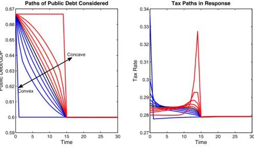
In particular, we focus on the impact of two important dimensions, namely the curvature of the debt/GDP path over the transition and the time span during which the debt/GDP ratio is reduced, on the welfare costs occurring over the transition.
To shed more light on these issues, we compute the overall welfare effects, i.e. the sum of welfare over the transition and in the final stationary equilibrium, for a small and realistic unanticipated reduction of the debt/GDP ratio from 0.66, the long-run average of the US, to 0.6. We assume that this reduction is financed by increasing the (linear) personal income tax rate, therefore keeping the distortions on asset and labor supply constant.
For all cases that we compute, we find that the transitional welfare costs associated with reducing government debt more than offset the long-run benefits of living in a stationary equilibrium with a lower debt/GDP ratio. This finding explains why debt reductions face so much political resistance, despite the fact that, according to our results, lower debt/GDP ratios are welfare-enhancing for the average household in the long run.3 Interestingly, we show that the government can minimize the welfare costs occurring over the transition by following a concave debt/GDP path, for which the reduction is initially slow and accelerating over time. The welfare losses can be further reduced by extending the time horizon during which public debt is decreased.
In order to understand the determinants of the transitional welfare effects, it is again important to consider the role of inequality. When choosing the curvature of the debt/GDP path, the government faces the following trade-off. On the one hand, a convex debt/GDP path offers the advantage of minimizing intertemporal distortions arising through asset income taxation. This is because a convex debt/GDP path implies that taxes are high at the beginning, when assets are pre-determined. On the other hand, households who are initially at the borrowing constraint prefer a concave debt/GDP path, for which the tax burden is initially low and increasing over time. The fact that in our calibration, consistent with the US economy, a substantial fraction of the population owns no assets or is in debt 3Protests can be fierce, as documented by Ponticelli and Voth (2011), who found that fiscal consolidation increases the likelihood of social unrest, in the sense of an organized resistance to the government (riots, demonstrations, political assassinations, government crises, and attempted revolutions).
explains why the concave path is superior to a convex or a linear path.4
In particular, our results about the importance of inequality for the transitional costs of debt re-ductions and inequality are consistent with the findings of D’Erasmo and Mendoza (2015), who study the link between domestic inequality and the likelihood to default on domestic debt in an incomplete markets model. They show that inequality increases the probability of default.
The previous literature has largely ignored welfare effects occurring over the transition altogether (see e.g. Aiyagari and McGrattan 1998 and Flod´en 2001). An exception is the work by Desbonnet and Weitzenblum (2011), who, however, do not match the large degree of wealth inequality observed in the data, which makes their stationary equilibrium results very different from ours. Moreover, they restrict their analysis of the transition to linear debt/GDP paths. Different from us, their focus is on computing the debt/GDP ratio that maximizes total (transitional plus stationary equilibrium) welfare, whereas we are interested in analyzing the welfare consequences of debt reduction policies. We contribute to this strand of literature by showing that inequality is important for welfare effects of government debt in the transition and in stationary equilibrium.
Apart from the aforementioned work, there are also other papers that study the effects of government debt in settings with incomplete markets. Gomes, Michaelides, and Polkovnichenko (2013) quantify the crowding out effect on the capital stock of a 10 percent increase in government debt in an incomplete market economy with aggregate risk. In a companion paper (Gomes, Michaelides, and Polkovnichenko 2012), the authors analyze the fiscal costs of the recent financial crisis in the US. Most recently, Azz-imonti, de Francisco, and Quadrini (2014) study a multi-country setting in order to explain the link between two trends that have been observed during the last three decades, namely the global rise in public debt and the liberalization of financial markets.
Our paper is also related to the work by A¸cikg¨oz (2014) and Dyrda and Pedroni (2015), who study the optimal Ramsey plan for a broad set of fiscal instruments in an environment with incomplete markets. In line with our findings, A¸cikg¨oz (2014) concludes the debt/GDP ratio that maximizes welfare in stationary equilibrium is negative. Similarly, Dyrda and Pedroni (2015) also find that the government should accumulate assets in the long run. Their results also indicate that, over the transition, it is optimal to tax capital income heavily, and to decrease labor income taxes in exchange.5
Following Aiyagari (1995), models with incomplete markets have been widely applied to study various aspects of fiscal policy. The welfare effects of capital taxation are studied by Domeij and Heathcote (2004) and Conesa, Kitao, and Krueger (2009), whereas Heathcote (2005) analyzes the impact of tax changes on aggregate consumption. Bakis, Kaymak, and Poschke (2015), Krueger and Ludwig (2013), and Kindermann and Krueger (2014) analyze the implications of tax progressivity. Instead, Angeletos and Panousi (2009), Challe and Ragot (2010), and Oh and Reis (2012) analyze the implications of various types of government expenditures for economic activity. In a recent paper, Bachmann et al. (2015) analyze the welfare and distributional effects of fiscal uncertainty using a neoclassical stochastic growth 4As a special case, we also consider the policy where the government unexpectedly raises the asset income tax in the initial period only. We find that in this case, government debt reductions lead to an overall welfare gain, which is however much smaller than the associated increase in stationary equilibrium welfare, implying that the transitional phase is still welfare-reducing. The reason is the existence of borrowing constraints. Because reducing public debt crowds in private capital, poor households, who depend largely on labor income, expect an increase in their income when public debt is decreased. As a result, they would like to borrow, which is only partially feasible. This leads to welfare losses.
model with incomplete markets. They show that the welfare gains of eliminating fiscal uncertainty decline with private wealth holdings. Their findings therefore also highlight the importance of matching inequality for understanding the consequences of fiscal policy. None of the aforementioned papers explicitly characterizes the welfare consequences of debt reductions in stationary state and over the transition.
The remainder of the paper is structured as follows. We present the baseline model in the next section. In Section 3 we discuss the calibration of the model. Section 4 shows the quantitative results, and Section 5 concludes.
2
The Baseline Model
The economy we consider is a neoclassical growth model with incomplete markets where households face uninsurable income shocks, as in Aiyagari (1994). The economy consists of three sectors: households, firms, and a government. In the following, we describe the three sectors in greater detail.
2.1
Household Sector
The economy is populated by a continuum of ex-ante identical, infinitely lived households with total mass of one. Households maximize their expected utility by making a series of consumption,ct, labor, lt, and savings,at+1, choices subject to a budget constraint and a borrowing limit on assets. In period t= 0, before any uncertainty has realized, their expected utility is given by:
U({ct,1−lt}t=1,2,...) =E0 ∞ X
t=0
βtu(ct,1−lt) (1)
where β is the subjective discount factor. The per-period utility function, u(.), is assumed to be strictly increasing, strictly concave, and continuously differentiable in both arguments.
Each household faces the following per-period budget constraint:
ct+at+1=yt+at (2)
whereat+1denotes the bond holdings of the household. ytis the household’s (after-tax) income from
labor and bonds. ytdepends, among other things, on the realization of a household-specific productivity
shock, denoted byt. We assume that t follows a Markov process with transition matrix π(t|t−1). Before we are able to fully characterizeyt, we need to describe the economy’s tax system, which will be
done when we introduce the government’s problem below.
Due to the presence of uninsurable productivity shocks, households self-insure against income fluc-tuations by saving in one-period risk-free bonds. Bonds can be issued by firms, the government, and other households (”IOUs”). Bonds issued by firms are claims to physical capitalKt. We abstract from
aggregate risk, which implies that all bonds are perfect substitutes, independent of the issuer, since they yield the same return, which we denote by 1 +rt.6
If households issue bonds,at+1 becomes negative. Households then borrow. Compared to Aiyagari and McGrattan (1998) and Flod´en (2001), we view this as an important modification, given that the 6In Gomes, Michaelides, and Polkovnichenko (2012, 2013), government bonds and private capital are imperfect substi-tutes due to aggregate uncertainty.
fraction of households that actually borrow in the data is substantial. For example, in the 2007 Survey of Consumer Finances (SCF), 24 percent of all households have a net financial asset position that is either zero or negative. We assume that borrowing is restricted:
at+1≥a (3)
In addition, we assume that the borrowing limit a is tighter than the natural borrowing limit, implying that it is binding for a certain fraction of the population.
The optimization problem of a household is given by the following functional equation:
Wt(a, ) = max c,l,a0 ( u(c,1−l) +βX 0 π(0|)Wt+1(a0, 0) ) (4) s.t. c+a0 = y+a (5) a0 ≥ a
The households’ problem is time-dependent because we do not only study stationary states but also transitions between them.7
2.2
Firm Sector
There is a continuum of firms operating a production technology that features constant returns to scale. Firms take prices on all markets as given. In competitive equilibrium, the number of firms is then indeterminate, and we can assume the existence of a representative firm. The representative firm produces output,Yt, by combining aggregate capital,Kt, and aggregate labor,Nt:
Yt=F(Kt, XtNt) (6)
whereXtdenotes exogenous labor-augmenting technological progress. Technological progress grows
at a constant rateg >0, such that Xt+1= (1 +g)Xt. By assuming that initial technology is given by X0= 1, the law of motion ofXtsimplifies toXt= (1 +g)t.
In order to obtain a stationary environment, we detrend all variables by dividing through Yt. The
detrended variables are denoted using a ”tilde”, e.g. Ket≡ KYt
t. In Appendix A , we outline the detrended
version of the households’ problem. There, we also illustrate that technological progress reduces the ”effective” discount factor, therefore implying that in the presence of technological progress, households are less willing to save.
2.3
Government Sector
We start by describing the balance sheet of the government. The government has to finance (exogenous) spending,Gt, transfers to households, denoted byT Rt, and interest payments for its outstanding debt,
which are given by rtBt. The government can raise income by issuing new government bonds, Bt+1, and by taxing income from assets and labor.
7Notice that as long we focus on the transition between stationary states, the dynamic programming problem of the household falls into the class of stationary dynamic programming problems, for which the principle of optimality is satisfied. We numerically show that our economy converges to a new stationary state.
More specifically, the tax system consists of proportional taxes on asset income,τk,t, a proportional
tax on labor income, τl,t, and a lump-sum transfer,χt. The results are affine taxes, which are a very
good approximation to the US tax code, according to Figure 1 in Bhandari et al. (2013). Proportional tax rates are given by a baseline component which is equal to the labor income tax rate,τt=τl,t, and
a premium on the asset income tax rate,ζ, such that ¯τk,t=ζτt. In our experiments, we will only vary
the baseline componentτt, keeping the premium on the asset income tax fixed.
Furthermore, we assume that only households with positive asset holdings are subject to the asset income tax, meaning that households in debt do not receive transfers that are proportional to their debt. More precisely, we define the tax rate on asset incomeτk,tas follows:
τk,t(a) = (
¯
τk,tifa≥0
0 ifa <0 (7)
The after-tax interest rate is therefore given byrt= (1−τk,t(a))rt. The after-tax wage rate is given
bywt= (1−τl,t)wt, wherewtis the price of labor in the economy. Total after-tax income is thus given
by:
yt=wtlt+rtat+χt (8)
The government budget constraint then reads as:
Gt+rtBt+T rt=Bt+1−Bt+τlwtNt+ ¯τkrtAbt (9)
whereAbt≥Atis the tax base for the asset income tax. Since taxes are levied only on positive financial
income, the tax base is defined as:
b At=
Z
a≥0
adθt(, a) (10)
whereθt(, a) denotes the distribution of households over income and asset states. Aggregate
trans-fers equal the sum of all individual transtrans-fers: Z
χtdθt(, a) =T rt (11)
Since the mass of households is normalized to one, and since χt is a lump-sum transfer that is
independent of the distribution of householdsθt(, a), individual transfers and aggregate transfers are
identical: χt=T rt.
Along a balanced growth path equilibrium, aggregate capital Kt, aggregate consumption Ct,
gov-ernment consumptionGt, public debt Bt, aggregate transfersT Rt, the aggregate tax baseAbt, and the
wage ratewt grow at the same constant rate g, while r and L are constant. Aggregate transfers are
given by T Rt = R
χtdθ(a, ), and the aggregate tax base is determined by ¯At = R
a≥0
atdθ(a, ). This
implies that the detrended versions of these variables, namelyKe,Ce,Ge,Be,T Rg,Aeb, andweare constant. We can then write the stationary version of the government’s budget constraint as follows:
e
G+ (r−g)Be+gT R=τlwNe + ¯τkrAeb (12) The stationary version of the government’s budget constraint will become important for the calibra-tion of our economy. Note that even when we compute the transicalibra-tion between two stacalibra-tionary equilibria, we keep the government spending/output ratioGe and transfer/output ratiogT R constant. This allows us to focus on the welfare effects of government debt and the timing of the (linear) taxes.
2.4
Competitive Equilibrium
Using the characterization of the three sectors we can now define the competitive equilibrium.
Definition 1.Competitive Equilibrium: Given a transition matrixπ, a government policy{Bt, τt, G}∞t=0,
and an initial distribution of the idiosyncratic productivity shocks and of the asset holdings θ0(, a), a recursive competitive equilibrium is defined by a law of motionΓ, factor prices{rt, wt}
∞
t=0, a sequence of value functions{Wt}∞t=0, and a sequence of policy functions {ct, lt, a0t}
∞
t=0 such that 1. Households solve the utility maximization problem as defined in equation (4). 2. Competitive firms maximize profits, such that factor prices are given by:
wt = FL(Kt, XtNt) (13)
rt = FK(Kt, XtNt)−δ (14)
3. The government budget constraint as defined in equation (12) holds. 4. Factor and goods markets have to clear:
• Labor market: Nt= Z ltdθt(, a) (15) • Asset market: At+1= Z a0tdθt(, a) =Kt+1+Bt+1 (16) • Goods market: Z ctdθt(, a) +Gt+It=F(Kt, XtNt) (17)
where investment I is given by:
I≡K0−(1−δ)K (18)
5. Rational expectations of households about the law of motion of the distribution of shocks and asset holdings, Γ, reflect the true law of motion, as given by:
θt+1(a, ) = Γ[θt(a, )] (19)
whereθt(a, )denotes the joint distribution of asset holdings and productivity shocks.
2.5
Welfare Measure
In order to be able to compare the welfare effects of different government policies, we have to define a welfare criterion. Following the previous literature, as for example, Aiyagari and McGrattan (1998) and Flod´en (2001), we compute the aggregate value function:
Ωt= Z
Wt(a, )dθt(a, ) (20)
This criterion can either be interpreted as (1) a Utilitarian social welfare function where every individual has the same weight for the planner, (2) a steady-state ex-ante welfare of an average consumer before
realizing income shocks and initial asset holdings, or (3) the probability limit of the utility of an infinitely lived dynasty where households’ utilities are altruistically linked to each other.
In order to facilitate the interpretation, we compute the average welfare change in consumption-equivalent units, i.e. the consumption that needs to be given to each household in order to make households indifferent on average between two specific policies.8 More details are provided in Appendix B.
3
Calibration
We calibrate the model such that it is consistent with long-run features of the US economy. The resulting allocation serves as a benchmark for our welfare calculations. Table 1 summarizes our parameter choices, which will be discussed in greater detail in the following subsections.
3.1
Utility Function and Production Technology
Utility function. We assume that preferences can be represented by a constant relative risk aversion
utility function:
u(c,1−l) = (c
η(1−l)1−η)1−µ
1−µ (21)
µdetermines the curvature of the utility function. We setµto 2. ηdenotes the share of consumption in the utility function. We calibrateη such that the average share of time worked, denoted by ¯l, is equal to 0.3. This results inη= 0.31.
Our parameter choices forµandη imply that the coefficient of risk aversion and the (average) Frisch elasticity of labor supply are both equal to 1.3.9 The coefficient of risk aversion is well in the range (between 1 and 3) commonly chosen in the literature. The Frisch elasticity is broadly in line with the outcome of other macro models in which the Frisch elasticity of the overall population is considered, but an order of magnitude larger than the Frisch elasticity estimated using micro data from prime age workers only.10
Before we proceed, a remark regarding the utility function is in order. Our specification is adopted from Aiyagari and McGrattan (1998). It is consistent with the existence of a balanced growth path. This requires that labor supply is subject to a wealth effect, such that hours worked remain constant, despite the fact that wages are permanently growing along a balanced growth path. This wealth effect will have consequences for some of our results discussed below.
In particular, it implies that the distribution of hours worked is inconsistent with the empirical evidence, see e.g. Casta˜neda, D´ıaz-Gim´enez, and R´ıos-Rull (2003). In the data, hours worked vary little, at least if one considers prime-aged individuals who work positive hours (see e.g. Pijoan-Mas 8More precisely, this measure provides the percentage increase in benchmark consumption at every date and state (with leisure at every date and state held fixed at benchmark values) that leads to the same welfare (under the benchmark policy) as under the new policy.
9For our specification of the utility function, the coefficient of risk aversion is given by 1−η+ηµ= 1.3. The Frisch elasticity of labor supply is given by (1−η+ηµ)/µ·(T−¯l)/¯l, whereT denotes the time endowment (normalized to 1 in our case) and ¯ldenotes the average fraction of time spend at work, in our case 0.3.
10The debate on whether micro and macro elasticities are consistent is ongoing. See Keane and Rogerson (2011) for a summary.
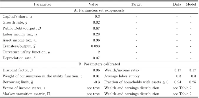
Table 1: Parameter Choices
Parameter Value Target Data Model
A. Parameters set exogenously
Capital’s share,α 0.3 - -
-Growth rate,g 0.02 - -
-Public Debt/output,Be 0.67 - -
-Labor income tax,τl 0.28 - -
-Asset income tax, ¯τa 0.36 - -
-Transfers/output,χe 0.083 - -
-Curvature utility function,µ 2 - -
-Depreciation rate,δ 0.07 - -
-B. Parameters calibrated
Discount factor,β 0.96 Wealth/income ratio 3.17 3.17
Weight of consumption in the utility function,η 0.31 Average labor supply 0.3 0.3
Borrowing limit, ˜a -0.3 Fraction of households with assets≤0 0.24 0.25
Vector of income states,s see text Wealth and earnings distribution see Table 2
Markov transition matrix, Π see text Wealth and earnings distribution see Table 2
Remarks: see main text for more details on the sources of parameters that are set exogenously and for calibration procedure of remaining parameters.
2006). Instead, the wealth effect inherent in our preferences commands that affluent households work less and enjoy their time in form of leisure.11 The model results for average hours worked by earnings quintile can be found in the Online Appendix.12
Technology. We now turn to the aggregate technology. We assume that it is given by a
Cobb-Douglas production function:
F(K, XN) =Kα(XN)1−α (22)
Initial technology is normalized toX0= 1, such thatXt= (1 +g)t. We setg= 0.02, which implies that
our economy grows at a rate of 2 percent per year. The parameterα, which denotes the share of capital in total production, is set to 0.3. This implies a labor share of 0.7. The discount factorβ is chosen such that the model reproduces a wealth/income ratio of 3.2, in line with e.g. Cooley and Prescott (1995) or ´Abrah´am and C´arceles-Poveda (2010).13
Finally, we set the annual depreciation rateδto 7 percent, which is a common value in the literature (see e.g. Trabandt and Uhlig 2011).
11We are grateful to the referees for pointing this out.
12The Online Appendix can be downloaded here: http://www.econ.uzh.ch/faculty/winter.html
13As we will explain in the subsection about the calibration of the income process, we define wealth as net financial assets. We measure the distribution of net financial assets in the 2007 SCF. As we will explain in the next subsection, compared to the 2007 SCF, our calibration generates too little wealth holdings at the very top of the distribution. We therefore pick 3.2 as a target for the wealth/income ratio, although the wealth/income ratio in the 2007 SCF is higher (3.7).
3.2
Taxes, Transfers and Government Debt
We now describe our choices for the tax rates, the transfers/GDP ratio, and the public debt/GDP ratio. Following Trabandt and Uhlig (2011), we set the labor income tax rate,τl, to 0.28 and the asset income
tax rate, ¯τk, to 0.36. This implies that the baseline component of our tax system is τl = τ = 0.28.
The relative premium of the asset income tax isζ≡ τ¯k
τ =
0.36
0.28. The values forτl and ¯τk describe the average (effective) tax rate on labor and capital income, respectively. They are computed from national income and product accounts (NIPA) for the US by dividing tax receipts from labor (capital) income by total labor (capital) income, as described in Mendoza, Razin, and Tesar (1994).14 Trabandt and Uhlig (2011) update the results of Mendoza, Razin, and Tesar (1994) for the period of 1995 to 2007. They find similar values, which suggests that average effective tax rates are stable over time.
We set the benchmark debt/GDP ratio, ˜B, to 0.66, following Aiyagari and McGrattan (1998), who define public debt as the postwar average of the sum of US federal and state debt. According to Trabandt and Uhlig (2011), average public debt/GDP was 0.63 for the period between 1995 and 2007, indicating that the debt/GDP ratio was roughly constant over time, at least prior to the recent financial crisis.
Lump-sum transfers/GDP, ˜χ, are set to 0.083, in accordance with both Aiyagari and McGrattan (1998) and Trabandt and Uhlig (2011), which again suggests that this ratio is fairly stable over time. In the data, transfers are calculated implicitly by subtracting government investment, interest rate expenditures, and government consumption from total expenditures, see Trabandt and Uhlig (2011).
Finally, government spending/GDP, ˜G, is the residual of the government’s budget constraint (12). In our model, a value of ˜G = 0.15 is needed in order to ensure a balanced budget. The appropriate empirical counterpart for ˜Gis the ratio of the sum of government consumption and investment to GDP. Aiyagari and McGrattan (1998) and Bachmann et al. (2015) report a ratio of government consumption and investment over GDP of 0.21 for the postwar period. Trabandt and Uhlig (2011) find a value of 0.18 for the period between 1975 and 2007. In either case, ˜G, as implied by our model, is smaller than its empirical counterpart. One reason could be that in our model, we abstract from consumption taxes. Allowing for consumption taxes (in addition to taxing labor and capital income) would increase total tax revenues, and would therefore allow the government to sustain a higher ˜G.
3.3
Income Process
We calibrate the vectorsof productivity realizationsand the corresponding transition matrix Π such that distributions of earnings and net financial assets generated by the model match their counterparts in the 2007 SCF. Our approach follows Casta˜neda, D´ıaz-Gim´enez, and R´ıos-Rull (2003). It is in part motivated by the fact that for standard parameterizations of the earnings process, incomplete markets models in the tradition of Aiyagari (1994) generate too little wealth inequality, compared to the data (see e.g. Quadrini and R´ıos-Rull 1997 or more recently Quadrini and R´ıos-Rull 2015).
Before we describe the calibration of the earnings process in greater detail, we explain how we mea-sure wealth and earnings. In our model, households accumulate assets to self-inmea-sure against idiosyncratic productivity shocks. We should therefore target those wealth holdings in the data that are accumulated for precautionary reasons as well. For this reason, we define wealth as net financial assets. More
cally, following ´Abrah´am and C´arceles-Poveda (2010), we calculate net financial assets by excluding the value of residential property, vehicles, and direct business ownership from total assets, and the value of secured debt due to mortgages and vehicle loans from total liabilities.15 In other words, we exclude those assets that are subject to adjustment costs and that are likely to serve a different role other than to transfer resources across time and states, such as housing and vehicles. Their adjustment is costly. Moreover, they are also used as consumption goods. Instead, financial assets can be readily sold to smooth out adverse productivity shocks.16
Earnings are defined as labor earnings (wages and salaries) plus a fraction of business income before taxes, excluding government transfers. This definition corresponds to the concept of earnings that is implied by our model.
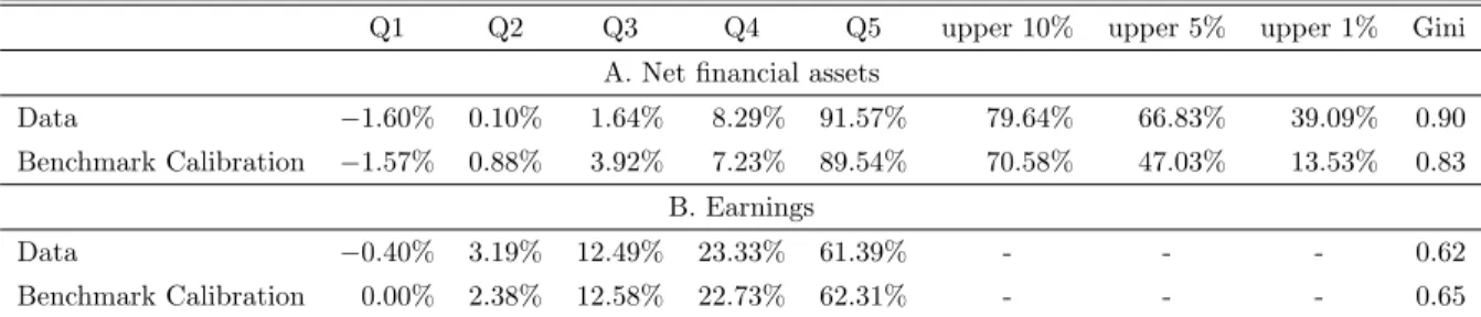
The distribution of earnings and net financial assets is computed from the 2007 SCF.17Table 2 shows that both earnings and net financial assets are very unequally distributed in the data. The richest 20 percent of the population hold more than 90 percent of all financial assets, net of debt. The distribution of earnings is less skewed. Households in the top quintile earn around 60 percent of the total earnings. We now turn to the details of our calibration procedure. Our strategy is to choose the vector sof productivity realizationsand the corresponding transition matrix Π such that distributions of earnings and net financial assets generated by the model match their respective distributions in the 2007 SCF. More specifically, for each unknown parameter, we pick one moment from the empirical Lorenz curve of either earnings or net financial assets. Since we assume that there are four productivity states, the corresponding transition matrix Π has 16 entries. We then normalize the mean of the productivity states to one. Because the transition probabilities in each row of Π have to sum up to one, we are left with 15 unknown parameters in total, 12 unknown transition probabilities and 3 unknown productivity states.
As targets, we choose the five quintiles and the Gini coefficients of the earnings distribution and the net financial asset distribution. We additionally target the top 10%, 5%, and 1% percentile of the distribution of net financial assets, in order to take into account that net financial assets are very unequally distributed within the upper quintile. However, we assign less weight to these targets, since the extremely skewed distribution of net financial assets makes it very difficult to match the top percentiles. This issue is well-known, see for example Table 14.6 in Quadrini and R´ıos-Rull (2015), which shows that other calibrations targeting the Lorenz curve of wealth also have difficulties to match the extreme right tail of the distribution. The 15 unknown parameters are then jointly chosen to match the 15 empirical moments.
15In terms of SCF variables, we calculate net financial assets as follows: Net Financial Assets = FIN - DEBT + MRTHEL + RESDBT + VEHINST.
16To what extent housing and consumption durables (and other illiquid assets) are used for consumption smoothing purposes is subject to an ongoing debate. See Fern´andez-Villaverde and Krueger (2011) and Kaplan and Violante (2010). Kaplan and Violante (2014) find that a significant fraction of those households that possess a large amount of net worth do not liquidate their assets due to transaction costs in response to temporary shocks and rather live ”hand-to-mouth,” which suggests that illiquid assets are not used to smooth consumption. See Heathcote, Storesletten, and Violante (2009) for a summary of the debate and additional references.
17The SCF does not specify the exact fraction of total business income that is attributable to labor and to capital. We define business income from sole proprietorship or a farm as labor earnings, whereas business income from other businesses or investments, net rent, trusts, or royalties is defined as capital income.
Table 2: Distribution of Net Financial Assets and Earnings, 2007 SCF and Benchmark Stationary Equilibrium
Q1 Q2 Q3 Q4 Q5 upper 10% upper 5% upper 1% Gini
A. Net financial assets
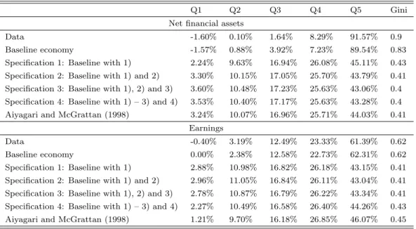
Data −1.60% 0.10% 1.64% 8.29% 91.57% 79.64% 66.83% 39.09% 0.90
Benchmark Calibration −1.57% 0.88% 3.92% 7.23% 89.54% 70.58% 47.03% 13.53% 0.83
B. Earnings
Data −0.40% 3.19% 12.49% 23.33% 61.39% - - - 0.62
Benchmark Calibration 0.00% 2.38% 12.58% 22.73% 62.31% - - - 0.65
Remarks: Quintiles (Q1-Q5) denote net financial assets (resp. earnings) of a group in percent of total net financial assets (resp. earnings). For the wealth distribution, in addition to the quintiles the table also shows the percent of net financial assets held by the wealthiest 10% (upper 10%), 5% (upper 5%), and 1% (upper 1%). The entries in ”data” are computed from the 2007 SCF. See main text for precise definitions. Notice that earnings can be negative due to the fact that labor earnings also contain part of the gains (or losses) of small enterprises.
As a result, we find the following vector of income states: s={0.055,0.551,1.195,7.351}
It should be noted that the highest income state is more than 130 times as high as the lowest income state.
Furthermore, we get the following transition matrix for the income states:
Π = 0.940 0.040 0.020 0.000 0.034 0.816 0.150 0.000 0.001 0.080 0.908 0.012 0.100 0.015 0.060 0.825
As indicated by the transition matrix, there is a 10 percent probability of moving from the highest productivity state today to the lowest productivity state tomorrow, which is associated with a large drop in earnings. This, in turn, generates a strong saving motive for income-rich households. The fact that income-rich households have both the opportunity and the incentive to accumulate large savings drives the unequal distribution of net financial assets in the model. Although the combination of specific values is somewhat arbitrary, the general mechanism is informative about how extreme actual saving motives and opportunities need to be in order to generate the observable distribution of net financial assets for the US economy only by self-insurance (Quadrini and R´ıos-Rull 2015).18
18Inequality might be partly determined by other factors that we abstract from such as entrepreneurship (Quadrini 1999 or Cagetti and De Nardi 2006), discount factor heterogeneity (as in Krusell and Smith 1998), life-cycle savings (see e.g. Huggett 1996), or non-homothetic bequest motives (as in De Nardi 2004). Gourinchas and Parker (2002) argue that a large fraction of non-pension wealth (up to 70 percent) in the US can be attributed to precautionary savings. As a robustness check, we repeated the first part of our welfare analysis (comparison of stationary equilibria associated with different public debt/GDP ratios) using the Krusell and Smith (1998) approach. Preliminary results, which are available from the authors upon request, suggest that our findings are qualitatively robust to using this very different approach of generating inequality.
3.4
Borrowing Limit
We calibrate the borrowing limit to match the percentage of households with negative or zero financial assets in the 2007 SCF (24 percent).19 We find a borrowing limit of ˜a = −0.3, which means that households can borrow up to 30 percent of output that is produced in the benchmark economy.
4
Results
We are now ready to compute the welfare effects of reductions in government debt. We distinguish between transition (in the following also labeled as short run) and stationary equilibrium (in the following also labeled as long run). We proceed in two steps. First, we analyze the welfare consequences of government debt reductions in stationary equilibrium. This is done by comparing stationary equilibria that are characterized by different debt/GDP ratios, keeping all other parameters constant. In order to keep the budget of the government balanced, we adjust taxes such that the relative distortions between capital and labor, denoted by ζ, remain constant. We find that in the long run, debt reductions are associated with welfare gains. In a second step, we also incorporate the welfare effects that occur over the transition between a high-debt stationary equilibrium to a low-debt equilibrium. We find that the costs of debt reductions occurring over the transition can be substantial, depending on the policy. The short-run costs of debt reductions can easily outweigh the long-run gains.
4.1
Effects of Public Debt in Stationary Equilibrium
In this section, we compute the long-run welfare-maximizing debt/GDP ratio in our economy. Our anal-ysis is motivated by the fact that in the textbook neoclassical model with lump-sum taxes, government debt is neutral and therefore has no impact on welfare. In a seminal paper, Aiyagari and McGrattan (1998) showed that in the presence of borrowing constraints and in the absence of complete markets, government debt has non-trivial welfare effects.
Two quantitative results from their paper have been very influential for the following research. First, Aiyagari and McGrattan (1998) argue that the debt/GDP ratio that maximizes long-run welfare is around 2/3, which is also the historical average of debt/GDP in the US economy. Second, they find that welfare effects of deviations from the long-run historical average are small.
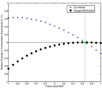
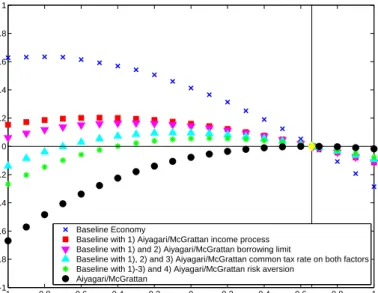
We show that these two conclusions drastically change in our calibration. In Figure 1, we plot the aggregate welfare changes for stationary equilibria for different public debt/GDP ratios, relative to the benchmark in which debt amounts to 2/3 of GDP. Figure 1 conveys a clear message: according to our calibration, stationary equilibria with lower debt/GDP ratios offer more aggregate welfare, compared to the benchmark. In our economy, the debt/GDP ratio maximizing long-run welfare is−0.8. Moreover, relative to the welfare function computed by Aiyagari and McGrattan (1998), our welfare function is much steeper around the long-run historical average debt/GDP ratio.
In the following, we analyze the driving forces behind the long-run welfare effects of changes in government debt in an Aiyagari (1994) style incomplete markets model in greater detail.
19Using the 2004 SCF, ´Abrah´am and C´arceles-Poveda (2010) find that 24.31 percent of households have negative or zero financial assets. This suggests that the this fraction is stable over time. To what extent our model generates a plausible number of borrowing-constrained households will be discussed in Footnote 25.
-1 -0.8 -0.6 -0.4 -0.2 0 0.2 0.4 0.6 0.8 1 -1 -0.8 -0.6 -0.4 -0.2 0 0.2 0.4 0.6 0.8 1 Public Debt/GDP
Welfare Change in Consumption Equivalents (in %)
Our Model Aiyagari/McGrattan
Figure 1:Comparing Welfare Between Different Stationary Equilibria.In this exercise we plot the welfare change in consumption-equivalent units implied by our baseline calibration (on the ordinate) for different stationary equilibria that differ with respect to the public debt/GDP ratio (on the abscissa), relative to the benchmark in which public debt amounts to 2/3 of GDP (green diamond and vertical line). Two cases: (1) Our Baseline Economy (blue crosses); (2) Aiyagari and McGrattan’s economy (black circles).
The long-run welfare effects of government debt result from the interaction between public debt and private capital. The interplay between public debt and private capital accumulation is a consequence of the fact that the borrowing constraint a is exogenous and fixed. Because of this, an increase in government debt crowds out private capital accumulation by effectively relaxing the borrowing limit (Woodford 1990, Aiyagari and McGrattan 1998).20
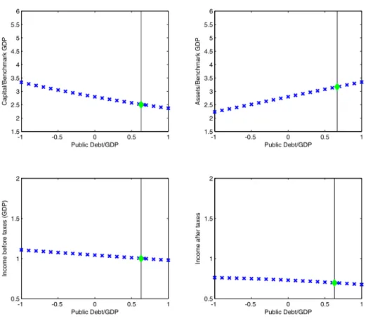
For our baseline calibration, the effect of public debt on private capital (private savings minus public debt) can be seen in Figure 2, where we depict assets (i.e. aggregate private savings) and the capital stock, relative to GDP.
Higher public debt/GDP ratios decrease capital. This means that the increase in assets demanded by households cannot compensate for the increase in assets supplied by the government. The reverse also holds. If government debt is reduced, the capital stock is crowded in. Households do not reduce their asset holdings as much as the government reduces its debt. As a result, the capital stock increases. If the capital stock in the baseline calibration is below its efficient level, the crowding in of capital increases welfare, all other things equal. In a recent paper, Davila et al. (2011) show that in an environment in which markets are incomplete, inequality, in particular the nature of the income risk as well as the composition of income for the consumption-poor, is an important determinant of the constrained efficient capital stock. Davila et al. (2011) show that if the earnings process is calibrated as in Casta˜neda, D´ıaz-Gim´enez, and R´ıos-Rull (2003) - the method that we employ in this paper - the constrained efficient capital stock is much higher than its laissez-faire level. This finding is in line with our result that government debt reductions increase the private capital stock and raise welfare.
20We study the relationship between public debt and borrowing limits in a separate paper, see R¨ohrs and Winter (2015). In the other project, we also allow for endogenous borrowing limits that result from a limited commitment problem.
-1 -0.5 0 0.5 1 1.5 2 2.5 3 3.5 4 4.5 5 5.5 6 Public Debt/GDP Capital/Benchmark GDP -1 -0.5 0 0.5 1 1.5 2 2.5 3 3.5 4 4.5 5 5.5 6 Public Debt/GDP Assets/Benchmark GDP -1 -0.5 0 0.5 1 0.5 1 1.5 2 Public Debt/GDP
Income before taxes (GDP)
-1 -0.5 0 0.5 1 0.5 1 1.5 2 Public Debt/GDP
Income after taxes
Figure 2: Capital, Assets, Income Before Taxes, Income After Taxes. This figure shows the changes in selected aggregate economic variables (on the ordinate) for different stationary equilibria that differ with respect to the public debt/GDP ratio (on the abscissa). In the benchmark, public debt amounts to 2/3 of GDP (green diamond and vertical line). All variables relative to GDP in the benchmark.
The interplay between government debt and private capital affects welfare through three channels, which we describe in more detail in the following.21
Level effect: Lower government debt/GDP ratios lead to more private capital and therefore to more
production (see the lower panel in Figure 2). To the extent that more capital and output translates into higher average consumption of goods and leisure, a lower debt/GDP ratio is welfare-improving. Follow-ing Flod´en (2001), we label the impact of government debt on average leisure-compensated consumption the ”level effect.” In general, we expect the level effect to be non-linear. Flod´en (2001) finds that the level effect is concave around the benchmark debt/GDP ratio. Since we use a different calibration of the earnings process, which is closer to Davila et al. (2011), we would expect that lower debt/GDP ratios (and hence more private capital), relative to the benchmark, are welfare-enhancing, at least to some extent.
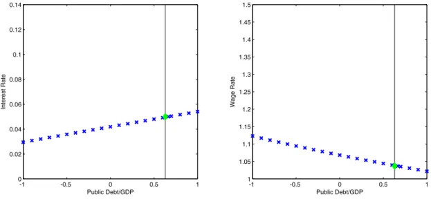
Insurance effect: There are two channels through which a decline in government debt affects households’ ability to self-insure. First, a decrease in public debt means that households effectively face tighter borrowing limits, because there is less liquidity that can be used to smooth consumption if households hit the constraint. Moreover, because reducing government debt crowds in private capital, we observe a decrease in the interest raterand an increase in the wage ratew(see Figure 3). This, by itself, increases the opportunity costs of households to self-insure against adverse productivity shocks. Put differently, precautionary saving becomes more costly.
-1 -0.5 0 0.5 1 0 0.02 0.04 0.06 0.08 0.1 0.12 0.14 Public Debt/GDP Interest Rate -1 -0.5 0 0.5 1 1 1.05 1.1 1.15 1.2 1.25 1.3 1.35 1.4 1.45 1.5 Public Debt/GDP Wage Rate
Figure 3:Interest Rate and Wage Rate.This figure shows the changes in equilibrium prices for capital and labor (on the ordinate) for different stationary equilibria that differ with respect to the public debt/GDP ratio (on the abscissa). In the benchmark, public debt amounts to 2/3 of GDP (green diamond and vertical line).
In addition, a fall in the interest rate and an increase in the wage rate increases uncertainty in total income, all other things equal. Imagine a household who receives income from labor and capital and who does not change its labor supply and its asset position. This household will experience an increase in uncertainty of total income since the weight of the uncertain income component, namely labor income, is increased relative to capital income, which is certain in our economy.22 As a result of higher uncertainty regarding total income, uncertainty about consumption is amplified as well, and households experience an ex-ante welfare loss. Note that capital income is only certain in our economy because we abstract from aggregate risk. Gomes, Michaelides, and Polkovnichenko (2008) analyze the impact of changes in government debt in a framework with infinitely-lived households, idiosyncratic and aggregate uncertainty. They argue that the presence of aggregate uncertainty amplifies the impact of changes in public debt on private capital and the interest rate.
Income composition effect: A reduction in government debt/GDP implies that the interest rater
falls, while the wage ratewincreases. As a consequence of these price changes, asset owners experience, on average, a loss in their income if there is more government debt, while those households who primarily depend on labor income, experience a gain. We call this the income composition effect. It is important 22Note that the aggregate income shares of capital and labor are constant, given our Cobb-Douglas specification. We are grateful to a referee for pointing this out.
to notice that the income composition effect would also exist if consumption was certain, in which case the insurance effect of government debt changes would be absent.
In sum, a reduction in government debt affects aggregate welfare in the long run via a level effect, an insurance channel, and through the composition of individual income. The impact of the level effect on aggregate welfare is ambiguous. The income composition effect implies that lower debt/GDP increases aggregate welfare, whereas the insurance effect implies that welfare decreases for lower debt/GDP ratios. The relative strength of each channel depends on the degree of wealth and income inequality in the economy. In the following paragraph, we will decompose the total welfare effect into its subcomponents.
Decomposition of Total Welfare Change. We now decompose the total welfare effect of public
debt into its subcomponents level, insurance, and income composition effect. In order to do so, we use the procedure outlined by Flod´en (2001), who in turn builds on work by Benabou (2002). The technical details of this decomposition can be found in Appendix C.
Since we are particularly interested in understanding the contribution of our earnings process, we conduct the following experiment. We compute aggregate welfare changes for two different economies, namely for our baseline economy and for a modified version of it, in which we replace our earnings process by the AR(1) process used in Aiyagari and McGrattan (1998).23 We re-calibrate the modified economy such that it is consistent with all targets of our baseline calibration (with the exception of wealth and earnings inequality). For both economies, we then decompose the total welfare effect of government debt changes into the level, insurance, and income composition effect.
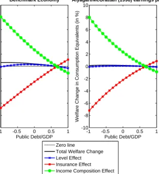
The results of this decomposition are shown in Figure 4. A comparison of the two economies reveals that the aggregate welfare function of government debt for the economy with the Aiyagari and McGrattan (1998) (panel to the right) earnings process is substantially flatter. Consequently, the public debt/GDP ratio that maximizes long-run welfare is larger (at around−0.5 instead of−0.8).
Figure 4 indicates sizable differences in the level effect between the two calibrations. In particular, our economy generates a stronger level effect for public debt/GDP ratios below the long-run average. According to Flod´en (2001), the level effect measures the change in (leisure-compensated) consumption of the average household following a change in government debt. Our results therefore imply that a reduction of public debt/GDP raises the leisure-compensated consumption of the average household by more if we use our income process instead of the income process employed by Aiyagari and McGrattan (1998). Leisure-compensated consumption, in turn, is determined by output (minus depreciation), rela-tive to hours worked (Heathcote, Storesletten, and Violante 2008). Since we use the same depreciation rates in the two experiments depicted in Figure 4, differences in the level effect must therefore be due to differences in the response of output/hours worked ratio across the two calibrations. In other words, our results indicate that if we use our income process, a reduction of government debt/GDP, relative to the long-run average, has a more pronounced effect on labor productivity.
In the following, we want to shed more light on the relationship between changes in public debt and labor productivity, which ultimately explains the relationship between government debt and leisure-compensated consumption, i.e. the level effect. We are particularly interested in understanding how this relationship is influenced by the calibration of the income process. To be more precise, recall that 23Aiyagari and McGrattan (1998) assume a persistence parameter of 0.6 and a standard deviation of innovations of 0.3.
-1 -0.5 0 0.5 1 -10 -8 -6 -4 -2 0 2 4 6 8 10 Benchmark Economy Public Debt/GDP
Welfare Change in Consumption Equivalents (in %)
-1 -0.5 0 0.5 1 -10 -8 -6 -4 -2 0 2 4 6 8 10
Aiyagari/McGrattan (1998) earnings process
Public Debt/GDP
Welfare Change in Consumption Equivalents (in %)
Zero line
Total Welfare Change Level Effect Insurance Effect Income Composition Effect
Figure 4:Welfare Decomposition. We plot the welfare change in consumption equivalent units implied by our baseline calibration (on the ordinate, left panel) and the baseline calibration where we replace our earnings process with the AR(1) process of Aiyagari and McGrattan (1998) (on the ordinate, right panel) for various stationary equilibria that differ with respect to the public debt/GDP ratio (on the abscissa), relative to the benchmark in which public debt amounts to 2/3 of GDP. We decompose total welfare (black solid line) into a level effect (blue line with crosses), an income composition effect (green line with circles), and an insurance effect (red line with squares).
in our setting, total outputY is determined byY =Kα(XN)1−α, whereK denotes aggregate capital
andN denotes total (effective) labor supply, which, in equilibrium, is given byN =R
ldθ(, a). For simplicity, we will ignore the role of the labor-augmenting technology progressXin our analysis, thereby implicitly assuming thatX= 1.
It follows that aggregate labor productivity, defined as average output per hours worked or Y R
ldθ(,a),
depends on aggregate capitalK and the strength of the correlation between and l at the household level. The correlation can therefore influence the size ofN (see Heathcote, Storesletten, and Violante 2008), even if aggregate hours workedR
ldθ(, a) remain constant.
To make things more precise, consider a tightening of the correlation between andl, in the sense that households that are subject to favorable productivity shocks increase their labor supply, whereas those that are subject to adverse productivity shocks reduce their hours worked. As we will see in greater detail below, such a change in the correlation between and l can be caused by a change in government debt (specifically, by the effect the change in public debt has on aggregate priceswandr). Let us further assume that only the distribution of hours worked changes, so that total hours worked remain constant. Due to the fact that more productive households increase their labor supply, whereas less productive households reduce their hours worked, we observe an increase inN, even though ag-gregate hours worked R
ldθ(, a) do not change. As a consequence, both aggregate labor and capital become more productive, indicated by the fact that both Y
R
ldθ(,a) and
Y
K increase. Therefore, as long
asR
the extent that government debt affectsKandN (without affectingRldθ(, a)), it will have an impact on aggregate labor productivity, which accounts for the level effect.
We now argue that a reduction in public debt/GDP, relative to the long-run level of 0.66, leads to a stronger increase in bothKandN (for fixed aggregate hours worked), if we use our earnings process instead of the one employed by Aiyagari and McGrattan (1998).
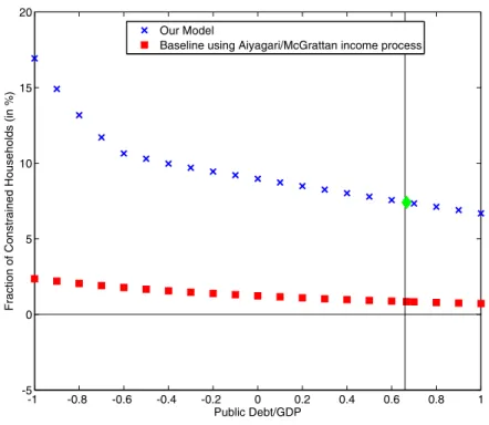
In order to understand the stronger response of aggregate capital, note that the fraction of households at the borrowing constraint is higher in our baseline calibration, as indicated by Figure 5. The fact that there are more constrained households implies more crowding in of private capital. The presence of constrained households leads to crowding in of private capital, since constrained households do not change their saving behavior in response to a reduction in public debt. As a consequence, a decline in government bondsB generates a situation in which the aggregate (net) demand for bonds (denoted by A) by private households exceeds the total supply of bonds (given byK+B). Here, K denotes bonds supplied by private firms to finance physical capital, andB denotes bonds supplied by the government. In order to achieve market clearing, a lower interest rateris required, which raises aggregate capitalK and therefore also the supply of bonds.
As a result of the increase inK, aggregate labor input becomes more productive when we consider a stationary equilibrium characterized by a lower debt/GDP ratio. Lower debt/GDP ratios are therefore not only associated with lower interest rates, but also with higher wage rates.
As a consequence of the aggregate price changes induced by a reduction in public debt/GDP, the correlation between labor supply and productivity shocks at the individual level becomes tighter if we reduce public debt/GDP. In order to understand why, note that our utility function, which we adopt from Aiyagari and McGrattan (1998), implies that individual labor supply is determined by a wealth and a substitution effect. For wealth-rich households, who are adversely affected by the decline in the interest rate, both wealth and substitution effect (stemming from the increase inw) leads to an increase in their supply of hours worked. Wealth-poor households instead depend mainly on labor income. For them, the increase in the wage rate constitutes a positive wealth effect, which partly offsets the substitution effect. As a result of these changes in labor supply across the wealth distribution, we get a tighter link between labor supply and wealth as we move to lower debt/GDP ratios.
In our economy, wealth is mainly determined by households’ desire to smooth consumption. Current wealth-rich households are also those that have received more favorable productivity shocks in the past. Wealth-poor households instead have been subject to adverse productivity shocks. To the extent that wealth-rich households are also earnings-rich in the sense that they currently receive a high productivity shock,24 the fact that the link between wealth and hours worked gets tighter at the household level for lower debt/GDP ratios also implies a tighter correlation between productivity shocks and hours workedlat the household level. This, in turn, increases N, all other things equal.
In conclusion, the fact that lower debt/GDP ratios crowd in private capital implies that aggregate labor is more productive. The increase in productivity is partly due to the higher aggregate private capital itself, and partly due to the tighter correlation between labor supply and productivity at the individual level, which raises the overall productivity. A a consequence, households can on average afford more consumption without having to increase their labor input, which explains why the level effect is 24This is quite likely, given the high degree of persistence in the transition matrix that governs the evolution of produc-tivity shocks.
positive for a certain range of public debt/GDP ratios below the long-run average. Moreover, because our calibration implies more crowding in of private capital (due to the presence of a larger fraction of households at the borrowing constraint), the level effect is more pronounced for our earnings process, compared to the process used by Aiyagari and McGrattan (1998).
Our discussion so far has implicitly assumed that the distribution of households remains constant, independently of the public debt/GDP ratio. This is of course not the case. As we show in Appendix D, there are substantial changes in the distribution of households. In particular, lowering public debt/GDP increases the fraction of poor households (defined as those without assets) and reduces the fraction of those that own assets. This finding is intuitive, given that stationary equilibria that are associated with lower public debt/GDP ratios are also characterized by a lower interest rate and a higher wage rate. As a result, the accumulation of savings is discouraged, and the fraction of poor households increases.
Changes in the distribution have important consequences for the relative strength of the various welfare effects. Consider, for example, the level effect. Because our preferences imply that labor supply is subject to a wealth effect, wealth-poor households work more hours than wealth-rich households. As a consequence, shifts in the distribution affect aggregate hours workedR
ldθ(, a). A larger fraction of wealth-poor households therefore leads to an increase in aggregate hours worked, which in turn reduces the output per hours worked and therefore leisure-compensated consumption, all other things equal.
Changes in the distribution therefore offer one explanation for the fact that the level effect is actually not monotonically increasing when we move to lower public debt/GDP ratios. As can be seen from Figure 4, the level effects starts to decline for debt/GDP ratios below−0.3. In this context, it is interesting to look at the development of the size of a particular subgroup of wealth-poor households, namely those at the borrowing constraint. Working more is the only option these households have in order to ameliorate the impact of the constraint on their consumption. Strikingly, the fraction of borrowing-constrained households is increasing drastically for small public debt/GDP ratios, as shown in Figure 5.25
We now analyze the insurance and the earnings composition effect in greater detail. Figure 4 indicates that the income composition effect is positive for debt/GDP ratios below the long-run average of 0.66. Rich households lose, whereas poor households win in the long run if the government reduces its debt. Instead, the insurance effect is negative for debt/GDP ratios below 0.66. Reducing government debt makes it more difficult for households to self-insure, due to the decline in the interest rate. The income composition effect appears to be somewhat weaker under the earnings process used by Aiyagari and McGrattan (1998), at least for debt/GDP ratios that are not too far away from the long-run average. However, it seems that the impact of our earnings process on the income composition effect is small.
Turning to the insurance effect of government debt, we find that its size depends on the earnings 25One might wonder whether the fraction of borrowing-constrained households depicted in Figure 5 is actually empirically plausible. It is difficult to assess to what extent borrowing constraints are binding in the data. One measure comes from the SCF, where households are asked whether, at any point in the last year, their credit application was turned down. In a separate question, households are asked whether they did not apply for credit because they feared that their application would be turned down. Jappelli (1990) identifies constrained households using these questions. In the 2007 survey, around 25 percent of households answered at least one of the two questions with yes, see Bricker et al. (2014). About 17 percent of all households reported that their credit application was actually turned down. These outcomes appear to be fairly stable across various SCF waves, see again Bricker et al. (2014). Compared to these measures, the fraction of constrained households generated by our model seems small, which suggests that our results provide a lower bound to the possible effects of government debt changes.
-1 -0.8 -0.6 -0.4 -0.2 0 0.2 0.4 0.6 0.8 1 -5 0 5 10 15 20 Public Debt/GDP
Fraction of Constrained Households (in %)
Our Model
Baseline using Aiyagari/McGrattan income process
Figure 5: Fraction of Households at the Borrowing Constraint. This figure shows the changes in the fraction of constrained households (on the ordinate) for different stationary equilibria that differ with respect to the public debt/GDP ratio (on the abscissa). In the benchmark, public debt amounts to 2/3 of GDP (green diamond and vertical line). Two cases: Our Model (blue crosses); Baseline using Aiyagari/McGrattan income process (red squares).
process. The impact of the earnings process on the strength of the insurance channel appears to be ambiguous, however. For debt/GDP ratios that are in the neighborhood of the long-run average of 0.66, our income process produces a stronger insurance effect. The opposite appears to be the case for debt/GDP ratios below−0.5. As a result, the income composition effect dominates the insurance effect in our benchmark calibration for debt/GDP ratios below−0.5, whereas both channels cancel out when we use the Aiyagari and McGrattan (1998) earnings process, independent of the debt/GDP ratio.
It turns out that the strength of the insurance channel can be approximated well by the development of the fraction of households at the borrowing constraint. As indicated by Figure 5, the path of the fraction of constrained households for both calibrations is also non-linear.
In particular, an increase in the public debt/GDP ratio from −1 to −0.5 reduces the fraction of constrained households by 50 percent in the modified economy (from 2 to 1 percent). The decline in the baseline calibration amounts to only 30 percent (from 17 to 11 percent). At the same time, Figure 4 reveals that the insurance effect is more pronounced for the modified economy within this range, relative to the baseline calibration.
The picture turns out to be completely different if we consider an increase in the debt/GDP ratio from −0.5 to 0.66. Here, the baseline calibration implies a decrease in the fraction of constrained households by 30 percent (from 11 to 7.5 percent), whereas the alternative calibration using the Aiyagari and McGrattan (1998) earnings process generates a decline of 20 percent (from 1 to 0.8 percent). Again, Figure 4 shows that the insurance effect is now more pronounced for the baseline economy, consistent with the stronger response in the fraction of constrained households.