Semiparametric methods for evaluating the covariate-specific predictiveness of continuous markers in matched case-control studies

(1)

UW Biostatistics Working Paper Series

5-25-2008

Semiparametric methods for evaluating the

covariate-specific predictiveness of continuous

markers in matched case-control studies

Ying Huang

Fred Hutchinson Cancer Research Center, [email protected]

Margaret S. Pepe

University of Washington, [email protected]

Suggested Citation

Huang, Ying and Pepe, Margaret S., "Semiparametric methods for evaluating the covariate-specific predictiveness of continuous markers in matched case-control studies" (May 2008).UW Biostatistics Working Paper Series.Working Paper 329.

(2)

1 Introduction

New technologies, such as gene expression microarrays and protein mass spectrometry, promise a multitude of biomarkers for detecting disease and predicting future events. Statistical methodology is needed to critically evaluate them. Biomarkers differ in their purposes and consequently demand different criteria for evaluation. For example, diagnostic markers are used to classify people as diseased or nondiseased. Their performance is typically evaluated with measures like sensitivity, specificity, and the ROC curve. Risk prediction markers, on the other hand, are utilized to predict the risk of having or getting a disease or other event. For risk prediction markers, measures that quantify their abilities to stratify risk are most relevant (Cook, 2007). Pepe et al. (2007) and Huang et al. (2007) proposed a graphical tool, the predictiveness curve to characterize the population distribution of predicted risk. LetDbe a binary outcome, andY be the markers of interest, and letRisk(y) = P(D= 1|Y =y) be the risk predicted for subjects with marker valueY =y. We write the predictiveness curveR(v) vsv, whereR(v) is the 100×vth _{percentile of}_Risk₍_Y_{). Equivalently we plot}

pvsFR(p), whereFR(p) is the cumulative distribution of risk in the population,R−1(p) =FR(p).

The distribution of Risk(Y) can be used to compare risk prediction markers or models. It provides a common scale for comparing models. A better model for risk stratification will have larger variability in risk percentiles. Equivalently, it will assign more subjects into low and high risk ranges.

As pointed out by Huang et al. (2007), the predictiveness of a marker depends on the target population. If there are covariates that define subpopulations, then a marker’s covariate-specific predictiveness should be explored in order to identify subpopulations where it is useful for risk stratification and subpopulations where it is not. Another motivation for considering covariate-specific curves is for individual decision making about having a marker measured or not. A subject may decide that it is valuable to ascertain the value of a marker for him/her only if there is a reasonably large chance that his/her risk calculated on the basis of marker and covariates will differ substantially from that calculated only on the basis of covariates. Covariate-specific predictiveness curves also address this question as we will illustrate.

There are two ways in which covariates can impact a marker’s predictiveness. Covariates may be predic-tors themselves, possibly interacting with the marker’s effect on risk. In other words, covariates can affect the shape and height of the risk as a function ofY. On the other hand, the distribution of the marker may

(3)

vary with covariates. Both effects impact on the distribution of risk, i.e. the predictiveness curve.

LetZ be covariates of interest, letRisk(Y, Z) =P(D= 1|Y, Z), then the covariate-specific predictiveness curve forY givenZ=zis the curveRz(v) vsv, whereRz(v) is the 100×vthpercentile ofRisk(Y, Z) in the

population with Z =z. Estimation of the covariate-specific predictiveness curve with data from a cohort design has been studied in Huang et al. (2007). Since case-control studies are more frequently conducted, particularly in the early phases of biomarker development (Pepe et al., 2001), it is important to develop estimators for this type of design as well. Here we consider case-control study designs. Moreover, our methods accommodate matching where controls are frequency matched to cases in regards to a subset of covariates.

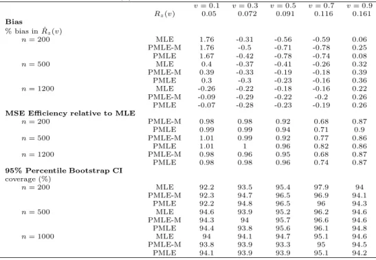
To fix ideas consider the following example of a study to evaluate serum creatinine as a predictor of risk of renal artery stenosis in patients with therapy resistant hypertension. A large cohort of subjects undergoing renal arteriography constitutes the patient cohort for a case-control study of serum creatinine. Details are provided in Section 4. Baseline risk of significant stenosis is calculated on the basis of several covariates including age, gender, smoking, etc. For illustration, we consider risk values above 0.4 as high enough to routinely recommend renal arteriography and risk values below 0.1 as low enough to discourage the practice. Figure 1 shows the predictiveness curves for serum creatine in subjects with baseline risk categorized as low, medium, and high. We see that among subjects originally deemed medium risk according to baseline factors, 24.8% are reclassified as low risk and 7.1% reclassified as high risk after including serum creatinine in the risk model. On the other hand, only a small fraction of subjects in the high or low risk categories according to baseline factors move to the medium risk designation after serum creatinine is included, and none move from the high risk to low risk category or vice versa. Therefore, on average ascertainment of serum creatinine seems to be most useful for subjects with medium baseline risk since in this group a substantial proportion are moved across risk thresholds that affect medical decisions. Cook (2007) proposed a simplified version of this sort of approach to evaluating the incremental value of C-reactive protein for cardiovascular risk assessment.

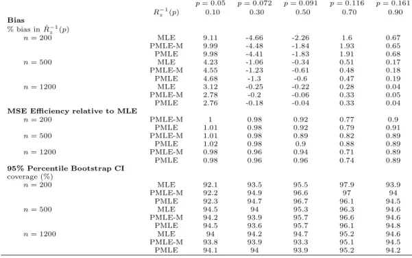
While predictiveness curves specific to baseline risk categories provide a big picture of the marker’s incremental value in terms of affecting medical decisions in subpopulations, another kind of predictiveness curve which is specific to an individual’s baseline covariate values is more useful for individual decision

(4)

making. In Figure 2 the covariate-specific curves are for individuals with specific values for the baseline covariates. For example, subject 2 has baseline risk equal to 38.1%. His predictiveness curve indicates that if serum creatinine is obtained from him, he has 0.5% chance of being classified as low risk. If his personal threshold for risk is low and he will opt for renal arteriography unless he is deemed to have risk<10%, there is no point in ascertaining serum creatine for him, because almost certainly his risk calculated with serum creatinine in addition to baseline covariates will exceed 10%.

In this paper we developed methodology to estimate and make inference about covariate-specific predic-tiveness curves, exemplified in Figures 1 and 2.

2 Method

We consider a case-control design where cases and controls are frequency matched withinS different strata. The special case where there is no matching corresponds toS= 1. Let S be the indicator for the matching stratum, taking values from 1 to S. We are interested in estimating the predictiveness curve for marker Y given values of covariateZ, assumingρs=P(D = 1|S =s), the disease prevalence within stratums is

apriori known. Consider the scenario where matching stratum S can be written as a function of Z, S(Z). An implication of this functional relationship between S andZ is that risk of disease conditional on marker Y and covariate Z is independent of stratum S. That is, P(D = 1|Y, Z, S) = P(D = 1|Y, Z), which we denote byG(θ, Y, Z), whereθis the risk model parameter. This is satisfied for example if strata are defined by a subset of covariates. Refer to the example in Section 1. Suppose samples are matched on baseline risk category, we haves= 1,2,3. MarkerY is serum creatinine. CovariateZ is baseline risk category in Figure 1 and baseline covariates in Figure 2.

Consider a logistic model where risk conditional on covariate value is monotone increasing as marker value increases

logit{P(D= 1|Y, Z)}= logit{G(θ, Y, Z)}=θ0+κ(θ1, Y, Z), (1)

where θ= (θ0, θ1)T. Here κ(θ1, Y, Z) is a pre-defined monotone increasing function forY givenZ =z. For

example,κ(θ1, Y, Z) might beθ11Y+θT12Z, the linear logistic model, or more flexiblyθ11Y(θ13)+θT12Z, where

Y(θ13)_{is the Box-Cox transformation (Cole and Green, 1992). Moreover, interaction between}_Y _and_Z_might

(5)

written as P(D= 1|Y, z) vsF−1

z (Y) where Fz(y) =P(Y ≤y|Z =z) is the CDF ofY whenZ =z. This

suggests estimation of the curve can be achieved in two steps: estimation of the risk model and estimation of the covariate-specific marker distribution. We take advantage of this in our proposed methods.

2.1 Discrete Covariate

Suppose the covariate of interest is discrete with Z categories. Let Z be the covariate group indicator, taking values from 1 toZ. For example, in a study where cases and controls are frequency matched by age subgroup, covariates of interest might be the combination of age subgroup and gender. A default strategy of estimating the predictiveness curve for marker Y within a particular covariate group is to use sample from that covariate group only. However, when risk model is not fully saturated (i.e. including main effects for all covariate categories and their interaction with the marker), borrowing information across covariate groups is more efficient.

Consider the risk model

logit{P(D= 1|Y, Z, S)}= logit{G(θ, Y, Z)}=θ0+θ1Y +θT2Z

M₊_θT

3Y Z

I_,

where θ = (θ0, θ1, θ2, θ3)T. Here ZM, ZI are vectors indexing subsets of covariate group. For example,

suppose covariateZ is the combination of age subgroup and gender, we can includeZM to index main effect for age subgroup and main effect for gender, and includeZI _{to index interaction between marker and gender}

only. The interaction terms vanishes whenZI _{is of length 0. Let}_L_R

zbe the likelihood ratio ofY conditional

on covariate valuez, which belongs to matching stratumS(z), we have

LRz(y) = P(Y =y|D= 1, Z=z) P(Y =y|D= 0, Z=z) = P(D= 1|Y =y, Z =z) P(D= 0|Y =y, Z =z) P(D= 0|Z=z) P(D= 1|Z=z) = expθ0+η(z) +θ1y+θ2Tz M₊_θT 3yz I _, ₍₂₎ whereη(z) = log{P(D= 0|Z=z)/P(D= 1|Z=z)}.

When the matching stratum S is the same as the covariate group, P(D = 1|Z = z) is known by assumption, and so is η(z). Consider now settings where the matching stratum is a proper subset of the covariate group. If information about P(D = 1|Z = z) is available, it can be directly utilized. However, if disease prevalence within a covariate group is not available,P(D= 1|Z=z) andη(z) can be estimated

(6)

from the case-control sample because by Bayes’ theorem, fors=S(z), η(z) = log _P₍_D_{= 0}_|_Z₌_{z, S}₌_s₎ P(D= 1|Z=z, S=s) = log P(D= 0|S=s) P(D= 1|S=s) + log P(Z=z|D= 0, S=s) P(Z=z|D= 1, S=s) = log ₁₋_ρ s ρs + log _P₍_Z₌_z_|_D_{= 0}_{, S}₌_s₎ P(Z=z|D= 1, S=s) , (3)

the first term in (3) is known, and for the second term, we can estimate P(Z = z|D = 0, S = s) and P(Z =z|D = 1, S=s) empirically from the case-control sample. Henceforth we use η(z) to represent the value that is known or estimated.

SupposenDcases andn_D¯ controls are sampled in the study. LetUsbe the set of subjects within matching

stratum swith UDs andU_Ds¯ being the subsets of cases and controls respectively. Leti index subject. We

maximize the empirical likelihood (Owen, 1988, 1990; Qin and Lawless, 1994) of observing the marker and the covariates values in the matched case-control sample.

Define Fz, FDz, andF_Dz¯ to be the cumulative distribution functions for marker Y in covariate groupz in

the general, diseased, and non-diseased populations. With a slight abuse of notation, let Uz be the set of

subjects within covariate groupzwithUDzandU_Dz¯ being the subsets of cases and controls respectively, and

(7)

in covariate groupz in the non-diseased population. Note that (4) can be rewritten as L(θ, F_Dz¯ ) = Z Y z=1    Y i∈UDz¯ dF_Dz¯ (Yi) Y i∈UDz dFDz(Yi)    = Z Y z=1    Y i∈UDz¯ dFDz¯ (Yi) Y i∈UDz LRz(Yi)dFDz¯ (Yi)    = Z Y z=1 ( Y i∈Uz dF_Dz¯ (Yi) Y i∈UDz LRz(Yi) ) = Z Y z=1 " Y i∈Uz piz Y i∈UDz expθ0+η(z) +θ1Yi+θT2ZiM+θ3TYiZiI #

subject to the restrictions piz > 0, Pi∈Uzpik = 1, and

P i∈UzpizLRz(Yi) = 1, for z = 1, . . ., Z. It is equivalent to maximize l = Z X z=1 X i∈Uz log(piz) + Z X z=1 X i∈UDz θ0+η(z) +θ1Yi+θT2Z M i +θ T 3YiZiI + Z X z=1 λ1z 1− X i∈Uz piz ! + Z X z=1 λ2z " X i∈Uz piz− X i∈Uz pizexpθ0+η(z) +θ1Yi+θT2Z M i +θ T 3YiZiI # , (5)

whereλ1z, λ2z are Lagrange multipliers.

Setting the first derivatives with respect to piz, θ2andθ0 to be zero, we get

∂l ∂piz = 1 piz −λ1z−λ2z expθ0+η(z) +θ1Yi+θT2Z M i +θ T 3YiZiI −1 = 0 ⇒ piz= 1 λ1z+λ2z expθ0+η(z) +θ1Yi+θT2ZiM+θT3YiZiI −1 , X i∈Uz ∂l ∂piz piz = nk−λ1z−λ2z+λ2z= 0 ⇒ λ1z=nz, ∂l ∂θ0 = nD− Z X z=1 λ2z X i∈Uz pizexp{θ0+η(z) +θ1Yi+θ2TZ M i +θ T 3YiZiI}= 0 ⇒ Z X z=1 λ2z=nD. (6)

Methods for solvingλ2zandθare derived in the appendix. In the special case whereZM is the covariate

group indicator, a closed-form solution does exist and the remainder of this section focuses on that special case. That is, supposeZM is a lengthZ −1 vector of dummy variables indicating covariate group, with the

(8)

ith_{element being}_I₍_Z ₌_i_{+ 1),}_i _{= 1,}_{. . .}_,_{Z −}_{1, we have} ∂l ∂θ2 = Z X z=1 X i∈UDz Zi− Z X z=1 λ2k X i∈Uz Z_iMpikexp{θ0+η(z) +θ1Yi+θT2Z M i +θ T 3YiZiI}= 0 ⇒ [λ2z]z=2,...,Z= Z X z=1 X i∈UDz ZiM= [nDz]z=2,...,Z. (7) Thusλ2z=nDz,z = 1,. . ., Z. We have piz= 1 n_Dz¯ +nDzLRz(Yi) = 1 n_Dz¯ +nDzexp n θ0+η(z) +θ1Yi+θ2TZiM+θ3TYiZiI o. Substitutingpiz into (5) we have

l = Z X z=1 X i∈Uz −logn_Dz¯ +nDzexp θ0+η(z) +θ1Yi+θT2ZiM+θ3TYiZiI + Z X z=1 X i∈UDz θ0+η(z) +θ1Yi+θ2TZ M i +θ T 3YiZiI .

Thus the maximum likelihood estimators ˆθ0, ˆθ1, ˆθ2and ˆθ3 solve

∂l ∂θ0 = nD− Z X z=1 nDz X i∈Uz expθ0+η(z) +θ1Yi+θ2TZiM+θT3YiZiI n_Dz¯ +nDzexp θ0+η(z) +θ1Yi+θ2TZiM+θT3YiZiI = 0, ∂l ∂θ1 = Z X z=1 X i∈UDz Yi− Z X z=1 nDz X i∈Uz Yi expθ0+η(z) +θ1Yi+θ2TZiM+θ T 3YiZiI n_Dz¯ +nDzexp θ0+η(z) +θ1Yi+θT2ZiM+θT3YiZiI = 0, ∂l ∂θ2 = Z X z=1 X i∈UDz ZiM− Z X z=1 nDz X i∈Uz ZiM expθ0+η(z) +θ1Yi+θT2Z M i +θ T 3YiZiI n_Dz¯ +nDzexp θ0+η(z) +θ1Yi+θ2TZiM+θT3YiZiI = 0, ∂l ∂θ3 = Z X z=1 X i∈UDz YiZiI− Z X z=1 nDz X i∈Uz YiZiI expθ0+η(z) +θ1Yi+θ2TZiM+θT3YiZiI n_Dz¯ +nDzexpθ0+η(z) +θ1Yi+θT2ZiM+θ3TYiZiI = 0,

Observe that these are the score equations if we fit a prospective logistic model

logit{P(D= 1|Y, Z)}=θ0+ξ(Z) +θ1Y +θT2Z

M₊_θT

3Y Z

I

to the case-control sample usingξ(z) = log (nDz/n_Dz¯ ) +η(z) as an offset term.

Therefore, to calculate the predictiveness curve specific for covariate group z, we first fit a prospective logistic model to the data and calculate ˆpiz, the maximum likelihood estimate of piz, i ∈ Uz. Then we

compute ˆ F_Dz¯ (y) = X i∈Uz ˆ pizI(Yi ≤y), ˆ FDz(y) = X i∈Uz ˆ pizI(Yi ≤y)LcRz(Yi),

(9)

where LcRz is the MLE ofLRz. We estimateFz as a weighted average of FDz andF_Dz¯ with weight being

P(D = 1|Z = z), disease prevalence within covariate group z. Note P(D = 1|Z = z) is either known or can be estimated as mentioned before. Let the estimate ofFz be ˆFz(y) =P(D= 1|Z=z) ˆFDz(y) +P(D=

0|Z=z) ˆF_Dz¯ (y). The semiparametric maximum likelihood estimator (MLE) of the predictiveness curve and

its inverse within covariate groupz are:

ˆ Rz(v) =G n ˆ θ,Fˆ_z−1(v), zo forv∈(0,1), ˆ R−_z1(p) = ˆFz n G−1θ, p, zˆ o forp∈ {Rz(v) :v∈(0,1)}, whereG−1₍_{θ, p, z}_{) =}_{_y_:_G₍_{θ, y, z}_{) =}_p_}_.

Observe that for the special case where ZI _{is also the covariate group indicator, we essentially allow for}

a different risk model within each covariate group, and our methods are equivalent to fitting the predictive-ness curve using the semiparametric two-sample MLE method (Huang, 2007) within each covariate group separately.

Based on similar arguments as in Huang (2007), asymptotic normality of ˆRz(v) and ˆR−z1(p) can be

derived. Proofs of the following theorems are outlined in the appendix.

Theorem 1

As n→ ∞,√nnRˆz(v)−Rz(v)

o

converges to a normal random variable with mean zero and variance

Σ1z(v) = _∂R z(v) ∂v 2 var√nhFˆz Fz−1(v) −v i + _∂R z(v) ∂θ T varn√n(ˆθ−θ)o ∂Rz(v) ∂θ + 2 _∂R z(v) ∂θ T cov√n(ˆθ−θ),√nhFˆzFz−1(v) −v i _∂R_z₍_v₎ ∂v . Theorem 2 Asn→ ∞,√nnRˆ−z1(p)−R −1 z (p) o

converges to a normal random variable with mean zero and variance

Σ2z(p) = var √ nhFˆz G−1(θ, p, z) −Fz G−1(θ, p, z) i + ∂R−z1(p) ∂θ T varn√n(ˆθ−θ)o ∂R −1 z (p) ∂θ + 2 ∂R−_z1(p) ∂θ T cov√nθˆ−θ,√nhFˆz G−1(θ, p, z) −Fz G−1(θ, p, z) i.

(10)

Observe that whenv=R−1 z (p), ∂R−z1(p) ∂θ ∂Rz(v) ∂v = ∂v ∂θ ∂Rz(v) ∂v = ∂Rz(v) ∂θ , thus Σ1z(v) ={∂Rz(v)/∂v} 2

Σ2z(p). That is the variance of ˆRz(v) and its inverse are related by a factor equal

to square of the derivative ofRz(v), which is intuitive since a perturbation inRz(v) can be approximated

byRz(v) times a perturbation inR−z1(p). In practice, bootstrap resampling is employed to assess sampling

variability, avoiding nonparametric density estimation.

2.2 Continuous Covariate

In Section 2.1, we developed an estimator of the covariate-specific predictiveness curve from a matched case-control study when covariates of interest are discrete. In this section, we investigate estimation in more general settings where continuous covariates can be involved.

Our strategy is to separate the estimation of the covariate-specific predictiveness curve into estimation of the risk model and estimation of the covariate-specific marker distribution. The first estimation can be achieved employing logistic regression model adjusted by the known disease prevalences within the matching strata. The second estimation can be performed using a weighted version of the semiparametric location-scale model (Heagerty and Pepe, 1999) for the marker distribution.

Consider the general risk model in (1). We apply a logistic model

logit{P(D= 1|Y, Z, S=s)}=θ0+ξ(s) +κ(θ1, Y, Z) (8)

to the case-control sample using

ξ(s) = log P(D= 1|S=s,sampled) P(D= 0|S=s,sampled) 1−ρs ρs

as the offset term, whereP(D= 1|S=s,sampled)/P(D= 0|S=s,sampled) is fixed by design and/or can be estimated in the case-control sample withnDs/n_Ds¯ .

Fitting this modified prospective logistic regression is essentially maximizing the “conditional (or pseudo) maximum likelihood” that an observation in the case-control sample within a particular stratum is a case or a control (Manski and Fadden, 1981; Hsieh et al., 1985; Breslow and Cain, 1988; Fears and Brown, 1986; Breslow and Zhao, 1988; Scott and Wild, 2001). Specifically, the contribution of subject i to the

(11)

pseudolikelihood is P(Di|Yi, Zi, Si,sampled). According to Bayes’ theorem, the odds of being diseased in

the case-control sample is

P(D= 1|Y, Z, S,sampled) P(D= 0|Y, Z, S,sampled) = P(Y, Z|D= 1, S,sampled) P(Y, Z|D= 0, S,sampled) P(D= 1|S,sampled) P(D= 0|S,sampled) = P(Y, Z|D= 1, S) P(Y, Z|D= 0, S) P(D= 1|S,sampled) P(D= 0|S,sampled) = P(D= 1|Y, Z, S)P(D= 0|S) P(D= 0|Y, Z, S)P(D= 1|S) P(D= 1|S,sampled) P(D= 0|S,sampled) = P(D= 1|Y, Z)P(D= 0|S) P(D= 0|Y, Z)P(D= 1|S) P(D= 1|S,sampled) P(D= 0|S,sampled) = exp{θ0+ξ(S) +κ(θ1, Y, Z)}.

Note that when the covariate of interest is the matching stratum, this pseudolikelihood approach leads to the same estimates of the risk model as in the MLE approach in Section 2.1.

For a more complicated design, the two-phase design, this pseudolikelihood method has been shown to be pretty similar to the maximum likelihood estimator which can be obtained by repeated fitting of ordinary logistic regression models (Wild, 1991; Scott and Wild, 1997; Breslow and Holubkov, 1997). Both estimators are shown to be much more efficient than the inverse probability weighted likelihood approach (Flanders and Greenland, 1991).

To estimate Fz, we employ a semiparametric location-scale model for the distribution of Y given Z

(Heagerty and Pepe, 1999). Suppose

Fz(y) =F0 _y₋_µ z σz ,

whereF0is the cumulative distribution function of some unknown distribution,µZ =γTU(Z) and log(σZ) =

δT_W₍_Z_{), and}_U₍_Z_{) and}_W₍_Z_{) are specified functions of} _Z_{. For example, for a discrete}_Z_,_U₍_Z_{) and}_W₍_Z₎

could be dummy variables indicating unique values ofZ, while for a continuousZ, they could be B-spline basis forZ. DenoteUi=U(Zi) and Wi=W(Zi). For a cohort study, Heagerty and Pepe (1999) proposed

estimatingγ andδ by solving the estimating equations

n X i=1 Ui(Yi−γTUi)/σ2Zi= 0, n X i=1 Wi (Yi−γTUi)2−σZ2i /σ 2 Zi= 0. (9)

(12)

(Horvitz and Thompson, 1952) version of these estimating equations in (9): n X i=1 1 ˆ qi Ui(Yi−γTUi)/σ2Zi= 0, n X i=1 1 ˆ qi Wi (Yi−γTUi)2−σ2Zi /σ 2 Zi = 0, (10)

where ˆqi= ˆP(sampled|Yi, Zi, Si, Di). Observe that

P(sampled|Yi, Zi, Si, Di) =P(sampled|Si, Di) =

P(Di|Si,sampled)P(Si|sampled)

P(Di|Si)P(Si)

,

where P(Di|Si,sampled) is fixed by design and can be estimated as well. So ifP(Si) is known in addition

toP(Di|Si), we can estimateP(Si|sampled) from the case-control sample and plug in

ˆ qi= ˆ P(Di|Si,sampled) ˆP(Si|sampled) P(Di|Si)P(Si) . Furthermore, we estimate F0by ˆ F0(c) = n X i=1 1 ˆ qi I Yi−ˆγTUi eδˆT_W_i ≤c ,_Xn i=1 1 ˆ qi .

The covariate-specific marker distribution estimate is ˆ Fz(y) = ˆF0 y−ˆγTu eˆδT_w ,

whereu=U(z) andw=W(z). The corresponding vth _{quantile is}

ˆ

F_z−1(v) = ˆγTu+eδˆTwFˆ₀−1(v) forv∈(0,1).

Estimators of the covariate-specific predictiveness curve forY givenZ =zwhich we call PMLE are ˆ Rz(v) =G n ˆ θ,Fˆ_z−1(v), zo forv∈(0,1), ˆ R−z1(p) = ˆFz n G−1(ˆθ, p, z)o forp∈ {Rz(v) :v∈(0,1)}.

Note that compared to the MLE method in Section 2.1, the PMLE method requires additional auxiliary information about the distribution of S. If the distribution of Y conditional on Z is independent of the matching stratumS, we can modify the PMLE method such that the extra piece of information aboutP(S) is not necessary. This is satisfied in current setting since S can be represented as a function of Z. The concept is to ensure unbiasedness of these estimating equations in (10) averaged across the distribution of Y within each stratum rather than averaged over the general population.

(13)

This way it is sufficient to adjust for selection bias within each stratum. For any two subjects i, j in the same stratum, we want to chooseqi andqj such that

qi/qj=P(sampled|Di, Yi, Zi, Si)/P(sampled|Dj, Yj, Zj, Sj).

GivenSi =Sj, we need to have

to guarantee the unbiasedness of (10) within each stratum. One of the choices ofqiisP(Di|Si,sampled)P(1−

Di|Si). We plug ˆqi= ˆP(Di|Si,sampled)P(1−Di|Si) into (10).

The covariate-specific predictiveness curve for marker Y can be derived likewise. We call the estimator PMLE-M. Note that PMLE and PMLE-M are equivalent when there is no matching in the case-control design. We use bootstrap resampling for variance estimation for both PMLE and PMLE-M estimators.

3 Simulation Studies

We evaluate our methodology using two simulation settings. In the first setting, cases and controls are frequency matched according to a binary covariate Z, which is also the covariate of interest for evaluating the marker’s predictiveness. MarkerY conditional onD andZ is normally distributed,

YD|Z= 0∼N(0.5,1), Y_D¯|Z= 0∼N(0,1),

YD|Z= 1∼N(1,1), YD¯|Z= 1∼N(0.5,1).

In the population, Z takes value 1 with probability 0.5. Disease prevalence given Z = 0,1 are 0.1 and 0.2 respectively. Within each matching stratum defined by the value of Z, equal number of cases and controls are sampled, and sample sizes are constant across strata. We compare the three estimators of the covariate Z-specific predictiveness curves developed in Section 2: the semiparametric MLE method assuming risk is linear logistic in Y andZ, and the PMLE and PMLE-M methods where location and log-scale parameters for the marker distribution are modeled as linear inZ.

(14)

Table 1: Performance of the covariate-specific predictiveness curve estimators for the first simulation setting in Section 3. Shown are results for ˆRz(v) withz= 0.

v= 0.1 v= 0.3 v= 0.5 v= 0.7 v= 0.9 Rz(v) 0.05 0.072 0.091 0.116 0.161 Bias % bias in ˆRz(v) n= 200 MLE 1.76 -0.31 -0.56 -0.59 0.06 PMLE-M 1.76 -0.5 -0.71 -0.78 0.25 PMLE 1.67 -0.42 -0.78 -0.74 0.08 n= 500 MLE 0.4 -0.37 -0.41 -0.26 0.32 PMLE-M 0.39 -0.33 -0.19 -0.18 0.39 PMLE 0.3 -0.3 -0.23 -0.16 0.36 n= 1200 MLE -0.26 -0.22 -0.18 -0.16 0.22 PMLE-M -0.09 -0.29 -0.22 -0.2 0.26 PMLE -0.07 -0.28 -0.23 -0.19 0.26

MSE Efficiency relative to MLE

n= 200 PMLE-M 0.98 0.98 0.92 0.68 0.87 PMLE 0.99 0.99 0.94 0.71 0.9 n= 500 PMLE-M 1.01 0.99 0.92 0.77 0.86 PMLE 1.01 1 0.96 0.82 0.86 n= 1200 PMLE-M 0.98 0.96 0.95 0.68 0.87 PMLE 0.98 0.98 0.96 0.74 0.87 95% Percentile Bootstrap CI coverage (%) n= 200 MLE 92.2 93.5 95.4 97.9 94 PMLE-M 92.3 94.7 96.5 96.9 94.1 PMLE 92.2 94.8 96.5 96 94.3 n= 500 MLE 94.6 93.9 95.2 96.2 94.6 PMLE-M 94.3 94 95.7 96.6 94.6 PMLE 94.4 93.8 95.6 96.1 94.8 n= 1000 MLE 94 94.1 94.7 95.1 94.6 PMLE-M 93.8 93.9 93.3 95 94.5 PMLE 94.1 93.9 93.9 95.1 94.2

andZ bivariate normally distributed with correlation 0.5 conditional onD,

Y Z D= 0∼N 0 0 , 1 0.5 0.5 1 , Y Z D= 1∼N 1 0 , 1 0.5 0.5 1 .

During the simulation cases are randomly sampled from the case population and for each case, a control with the sameZ value is generated. We again compare the three estimators of covariateZ-specific predictiveness curves. For the semiparametric MLE estimator, risk is modeled as linear logistic in Y and discretized Z (where cutoff points are chosen to be quintiles ofZ in the case population). For the PMLE and PMLE-M estimators, location and log(scale) parameters for the marker distribution are modeled as linear inZ.

For sample size varying from 200 to 1200, we evaluate estimates ofRz(v) andR−z1(p) forv= 0.1,0.3,0.5,0.7,0.9

and correspondingp=Rz(v).

For the first setting, simulation results forZ = 0 are presented in Tables 1 and 2. For the second setting, simulation results for Z equal to the median in the case population are presented in Tables 3 and 4. We find that in both settings the three estimators have reasonably good performance. Bias was minimal for Rz(v) and forR−z1(p). Coverage of the 95% confidence intervals constructed from the bootstrap distribution

(15)

Table 2: Performance of the covariate-specific predictiveness curve estimators for the first simulation setting in Section 3. Shown are results for ˆR−1

z (p) withz= 0. p= 0.05 p= 0.072 p= 0.091 p= 0.116 p= 0.161 R−_z1(p) 0.10 0.30 0.50 0.70 0.90 Bias % bias in ˆR−1 z (p) n= 200 MLE 9.11 -4.66 -2.26 1.6 0.67 PMLE-M 9.99 -4.48 -1.84 1.93 0.65 PMLE 9.98 -4.41 -1.83 1.91 0.68 n= 500 MLE 4.23 -1.06 -0.34 0.51 0.17 PMLE-M 4.55 -1.23 -0.61 0.48 0.18 PMLE 4.68 -1.3 -0.6 0.47 0.19 n= 1200 MLE 3.12 -0.25 -0.22 0.28 0.04 PMLE-M 2.78 -0.2 -0.06 0.33 0.05 PMLE 2.76 -0.18 -0.04 0.33 0.04

n= 200 PMLE-M 1 0.98 0.92 0.77 0.9 PMLE 1.01 0.98 0.92 0.79 0.91 n= 500 PMLE-M 1.01 0.98 0.89 0.82 0.89 PMLE 1.02 0.98 0.9 0.88 0.89 n= 1200 PMLE-M 0.98 0.96 0.94 0.71 0.89 PMLE 0.98 0.96 0.96 0.74 0.89 95% Percentile Bootstrap CI coverage (%) n= 200 MLE 92.1 93.5 95.5 97.9 93.9 PMLE-M 92.2 94.9 96.6 97 94 PMLE 92.3 94.7 96.7 96.1 94.5 n= 500 MLE 94.5 94 95.3 96.3 94.6 PMLE-M 94.2 93.9 95.7 96.6 94.6 PMLE 94.5 93.6 95.7 96.1 94.8 n= 1200 MLE 94 94.2 94.7 95.2 94.6 PMLE-M 93.8 93.9 93.3 95.1 94.5 PMLE 94.1 94 93.9 95.2 94.2

Table 3: Performance of the covariate-specific predictiveness curve estimators for the second simulation setting in Section 3. Shown are results for ˆRz(v) withzbeing the median ofZ in the case population.

v= 0.1 v= 0.3 v= 0.5 v= 0.7 v= 0.9 Rz(v) 0.022 0.054 0.097 0.173 0.358 Bias % bias in ˆRz(v) n= 200 MLE 12.21 3.85 0.01 -0.72 0.14 PMLE-M 3.53 0.63 -1.24 -0.4 -0.06 PMLE 3.87 0.91 -0.88 -0.18 0.04 n= 500 MLE 7 2.77 0.58 0.14 -0.63 PMLE-M 0.22 -0.58 -0.81 -0.22 0.52 PMLE -0.05 -0.7 -0.91 -0.34 0.61 n= 1200 MLE 7.24 3.97 1.89 0.22 -1.04 PMLE-M 0.36 -0.13 -0.36 -0.09 0.13 PMLE 0.33 -0.19 -0.3 -0.08 0.06

n= 200 PMLE-M 1.77 1.61 2.03 2.86 1.81 PMLE 1.8 1.58 1.82 2.12 1.51 n= 500 PMLE-M 1.98 1.82 1.84 2.75 1.76 PMLE 1.92 1.77 1.68 2 1.41 n= 1200 PMLE-M 2.19 2.02 2.01 2.69 1.78 PMLE 2.12 1.95 1.81 2.01 1.54 95% Percentile Bootstrap CI coverage (%) n= 200 MLE 96.1 96.8 97.2 98.7 98.7 PMLE-M 94.3 94.2 94.2 98.2 96.9 PMLE 93 91.6 92.4 95.5 97.9 n= 500 MLE 95.1 95.5 96.2 98.8 96.9 PMLE-M 93.8 93.7 93.5 97.7 95.1 PMLE 92.3 91.9 90.9 95.7 95.9 n= 1200 MLE 94.8 94 94.7 97.5 95.8 PMLE-M 94.2 94.1 94.9 96.2 95.7 PMLE 93.3 91.8 91.1 93 96.6

(16)

Table 4: Performance of the covariate-specific predictiveness curve estimators for the second simulation setting in Section 3. Shown are results for ˆR−z1(p) withzbeing the median ofZ in the case population.

p= 0.022 p= 0.054 p= 0.097 p= 0.173 p= 0.358 R−_z1(p) 0.10 0.30 0.50 0.70 0.90 Bias % bias in ˆR−1 z (p) n= 200 MLE 0.13 -2.62 -0.84 -0.01 0.46 PMLE-M 6.63 -0.56 0.12 0.11 0.33 PMLE 6.82 -0.65 0.06 0.0004 0.28 n= 500 MLE -2.61 -2.39 -0.72 -0.09 0.24 PMLE-M 5.11 0.86 0.28 0.05 -0.05 PMLE 5.09 0.99 0.35 0.13 -0.04 n= 1200 MLE -7.26 -3.73 -1.47 -0.18 0.31 PMLE-M 1.53 0.24 0.12 0.04 0.03 PMLE 1.54 0.23 0.13 0.05 0.02

n= 200 PMLE-M 1.47 1.75 2.13 3 1.83 PMLE 1.45 1.64 1.91 2.29 1.63 n= 500 PMLE-M 1.61 1.76 2.09 3.06 1.71 PMLE 1.54 1.71 1.89 2.19 1.45 n= 1200 PMLE-M 1.7 1.95 2.07 2.73 1.68 PMLE 1.67 1.87 1.86 2.03 1.45 95% Percentile Bootstrap CI coverage (%) n= 200 MLE 96.1 96.7 97.2 98.8 98.7 PMLE-M 94.2 94.2 94.2 98.3 96.9 PMLE 93 91.6 92.4 95.5 97.9 n= 500 MLE 95.1 95.5 96.2 98.7 96.9 PMLE-M 93.6 93.7 93.7 97.7 95 PMLE 92.7 91.7 90.9 95.7 95.9 n= 1200 MLE 94.8 94 94.7 97.4 95.8 PMLE-M 94.2 94.1 95 96.2 95.6 PMLE 93.4 91.7 91.2 93 96.6

is fairly close to the nominal level. In the first setting where there are two covariate groups, MSE for the three estimators are similar in magnitude. The MLE estimator is slightly more efficient than the PMLE and PMLE-M estimators for certain v. As the number of (discretized) covariate groups increases to five (the second setting), the MLE estimator becomes much less efficient compared to the PMLE and PMLE-M estimators.

Since the MLE method requires less model assumption, it is more robust than the PMLE (PMLE-M) methods. In practice the MLE method is preferred when the number of covariate groups is relatively small and the number of observations in each group is not too small, e.g. when covariate is baseline risk category in the renal example. On the other hand, since the PMLE (PMLE-M) methods borrow information across covariate groups during estimation of the marker distribution, it is expected to be more efficient compared to the MLE method as the number of covariate groups increases. Specifically, when we have several continuous covariates, like those baseline covariate values described in the renal example, the job to discretize these covariates for MLE estimation becomes very difficult and the PMLE (PMLE-M) methods are more appealing in this scenario.

(17)

0.0 0.2 0.4 0.6 0.8 1.0 0.0 0.2 0.4 0.6 0.8 1.0

Baseline Risk Specific Predictiveness Curve

v

R(v)

Low Risk Equivocal Risk High Risk

Figure 1: Predictiveness curves for serum creatinine specific to patients with low, high, and equivocal baseline risk. 0.0 0.2 0.4 0.6 0.8 1.0 0.0 0.2 0.4 0.6 0.8 1.0

Covariate Specific Predictiveness Curve

v

R(v)

Subject 1 Subject 2 Subject 3

Figure 2: Examples of covariate-specific predictiveness curves for serum creatinine.

4 Illustration

We illustrate the methodology evaluating serum creatinine as a risk prediction marker for renal artery stenosis in patients with therapy resistant hypertension. The original cohort consists of 426 hypertensive patients undergoing renal angiography (Janssens et al., 2005; Krijnen et al., 1998). Baseline risk is modeled with age, smoking status (ever) and their interaction, gender, hypertension, BMI, abdominal bruit, atherosclerosis disease, and hypercholesterolaemia. Consider a low risk threshold of 0.1 below which no routine angiography is recommended and a high risk threshold of 0.4 above which routine angiography is encouraged. There are 162 subjects in the cohort with low baseline risk (10 cases), 176 subjects with medium baseline risk (33 cases), and 88 subjects with high baseline risk (55 cases). A stratified case-control sample of size 217 is

(18)

generated including all 98 cases and controls frequency matched according to baseline risk group. Within low and medium baseline risk strata, the number of controls selected are twice that of cases, while within the high risk group, all controls are selected.

Figure 1 displays the predictiveness curves for serum creatinine, for patients within different baseline risk strata. Hence the covariate is baseline risk stratification, the same as the matching stratum. The MLE method was employed in estimation. Observe that for those patients who have low baseline risks, after measuring serum creatinine, there is ˆR−z1(0.1) = 94.5% chance that they will remain classified as low risk

(with 95% CI (94.8%, 100%)), a small chance that their risk will be elevated to the intermediate risk range ( ˆR−z1(0.4)−Rˆ

−1

z (0.1) = 5.2% with 95% CI (0, 24.0%)), and a negligible chance that their estimates risks

will be high enough to receive treatment recommendation (1−Rˆ−_z1(0.4) = 0 with 95% CI (0,0)). For those patients who are originally in the medium risk range, after measuring serum creatinine, they have 24.8% chance of being reclassified as low risk (with 95% CI (2.3%,42.8%)), 7.1% chance of being reclassified as high risk (with 95% CI (0.8%, 14.6%), and 68.1% chance of remaining in the risk grey zone (95% CI (43.4%, 95.4%)). For those patients whose baseline risk is high, if their serum creatinine levels are measured, their estimated risks have 90.9% chance of remaining high (with 95% CI (80.7%,97.7%)), 9.1% chance of being medium (with 95% CI (2.3, 19.3%)), and almost zero chance of being low enough such that treatment is deemed unnecessary (with 95% CI (0,0)). Note that for individuals originally in the medium risk range, measuring serum creatinine makes it easier for physicians to make recommendation about their subsequent medical procedures, whereas it is the other way around for those with low or high baseline risks.

For individual patients, detailed information about one’s baseline covariate values is more informative than the risk group one belongs to. Not only do individual baseline risks vary within a baseline risk category but also the new marker’s distribution may depend on the baseline covariates. Whenever information about baseline covariates are available, the covariate-specific predictiveness curve can be used to tailor a patient’s view about worthiness of having an extra test. To illustrate this, we display covariates-specific predictiveness curves for three individuals using the PMLE method (Figure 2). Results based on PMLE-M method are fairly similar (omitted). Subject 1 is a 57 years old female with BMI 26.8kg/m3 who has a smoking history,

hypertension and hypercholesterolaemia. Her baseline risk is 25.6%. Subject 2 is a 65 years old male with BMI 26.0kg/m3who has atherosclerosis disease. His baseline risk is 38.1%. Subject 3 is a 57 years old female

(19)

with BMI 22.2kg/m3_{who has smoking history and atherosclerosis disease. Her baseline risk is 42.6%. Next}

we look closely at the impact of measuring serum creatinine on each patient.

Subject 1 has her baseline risk in the middle of the equivocal range. If serum creatinine is included in the risk calculation, she has 8.6% chance of being reclassified as low risk (with 95% CI (0%, 50.1%)), 11.9% chance (95% CI (2.6%, 47.0%)) of being reclassified as high risk, and 79.5% chance (95% CI (36.8, 89.0%)) of remaining in the equivocal zone. Subject 2 is originally at the high end of the equivocal risk range. If his serum creatinine level is measured, he has 0.5% chance of being declared as low risk (with 95% CI (0%, 10.7%)), 50.7% chance (95% CI (10.5%, 84.5%)) of remaining in the risk grey zone. At the same time, there is 50.7% chance (95% CI (10.5%, 84.5%)) that he will be classified as high risk and receive recommendation for treatment. Subject 3 has her baseline risk marginally above high risk threshold. By measuring serum creatinine, there is almost zero possibility (with 95% CI (0, 5.6%)) that she will be classified as low risk; there is 69.4% chance (95% CI (25.6%, 95.0%)) that her risk will remain high and 30.6% chance (95% CI (25.6%, 95.0%)) that her risk will be deemed inadequate for making recommendation for or against treatment.

A subject’s choice about whether or not to measure a new marker will be affected by the marker’s potential impact on medical decisions as can be seen from the subject’s covariate-specific predictiveness curve. The specific risk thresholds on the curve pertinent to an individual will depend on beneficial and side effects of treatment, as well as one’s tolerance for the risk of the disease. In addition, the cost of measuring the raw marker may enter. For example, if subject 3 has a low tolerance for risk of disease and is willing to have routine angiography unless her risk is below 10%, she might choose not to measure serum creatinine since it is highly unlikely that her estimated risk will go below 10% based on the extra test. For subject 2, if he has low tolerance for risk, he might also choose not to measure serum creatinine since the chance for his estimated risk to drop below 10% is small; but on the other hand, if he has relatively high tolerance for risk and is willing to go through renal angiography only if his risk is above 40%, then measuring serum level might be attractive to him considering the large possibility that he will have a risk calculated that allows him to decide with confidence to have renal angiography.

(20)

5 Discussion

In this article we developed methodology for estimating the covariate-specific predictiveness curve for a single marker in a case-control study. Our method accommodate matching in design. Two types of semi-parametric approaches are examined assuming risk is monotone increasing in the marker value. The first approach is based on empirical likelihood ofY and is applicable to discrete covariates. The method can be easily generalized to the setting when Y is multivariate by modeling the empirical likelihood ofRiskz(Y)

following similar arguments as in Huang (2007). Note that another related estimator can be constructed by estimatingFDz andF_Dz¯ empirically using the case or control sample within thezthcovariate group. Since

the exponential tilt relationship (2) implied by the risk model is not incorporated into estimation of the marker distribution, this estimator is probably less efficient than the MLE. This has been demonstrated for the overall predictiveness curve estimated with a case-control study (Huang, 2007).

The second approach combines estimation of the risk model with estimation of the covariate-specific marker distribution assuming a semiparametric location-scale model forY. Different weighting schemes can be applied to accommodate the biased sampling design. This approach is applicable to general settings and is analogous to the semiparametric approach proposed in Huang et al. (2007) for a cohort design. For a generalization of this method whenY is multivariate, we can obtainRisk[(Yi), i= 1, . . . , nusing say

pseudo-maximum likelihood method, and then estimate the covariate-specific distribution ofRisk(Y) by plugging

[

Risk(Yi) into the weighted semiparametric location-scale model for logit{Risk(Y)}.

Note that from a matched case-control biomarker study, there are other types of predictiveness curves we might be interested in estimating besides the covariate-specific predictiveness curve investigated here. For example, we might be interested in the predictiveness curve based on both the biomarker and the covariates. Alternatively, we might want to investigate the covariate-adjusted predictiveness curve for the marker, characterized by a weighted summary of the covariate-specific predictiveness curves with weights related to the covariate distribution. These different types of predictiveness curves can be used to answer different scientific questions. Estimation of these predictiveness curves in a matched case-control study can be achieved by combining estimates of the covariate-specific predictiveness Rz(v) vs v and some extra

(21)

Acknowledgments

The authors are grateful for support provided by NIH grants GM-54438 and NCI grants CA86368.

References

Breslow, N. E. (1996). Statistics in epidemiology: the case-control study.JASA91,14-28.

Breslow, N. E. and Day, N. E. (1993).Statistical Methods in Cancer Research: The Analysis of Case-Control Studies. IARC.

Breslow, N. E. and Cain, K. C. (1988). Logistic regression for two-stage case-control data.Biometrika75(1),

11-20.

Breslow, N. E. and Holubkov, R. (1997). Maximum likelihood estimation of logistic regression parameters under two-phase, outcome-dependent sampling.J. R. Statist. Soc. B 59(2),447-461.

Breslow, N. E. and Holubkov, R. (1997). Weighted likelihood, pseudo-likelihood and maximum likelihood methods for logistic regression analysis of two-stage data.Statistics in Medicine 16,103-116.

Breslow, N. E. and Zhao, L. P. (1988). Logistic regression for stratified case-control studies.Biometrics 44,

891-899.

Cole, T. J. and Green, P. J. (1992). Smoothing reference centile curves: The LMS method and penalized likelihood.Statistics in Medicine 11(165),1305-1319.

Fears, T. R. and Brown, C. C. (1986). Logistic regression methods for retrospective case-control studies using complex sampling procedures. Biometrics,42,955-960.

Flanders, W. D. and Greenland, S. (1991). Analytic methods for two-stage case-control studies and other stratified designs.Statistics in Medicine, 10,739-747.

Cook, N. R. (2007). Use and misuse of the receiver operating characteristic curve in risk prediction. Circu-lation 115,928-935.

Heagerty, P. J. and Pepe, M. S. (1999). Semiparametric estimation of regression quantiles with application to standardizing weight for height and age in U.S. children.Applied Statistics 48,553-551.

(22)

Horvitz, D. G. and Thompson, D. J. (1952). A generalization of sampling without replacement from a finite universe.JASA47,663-685.

Hsieh, D. A. and Manski, C. F. and McFadden, D. (1985). Estimation of response probabilities from aug-mented retrospective observations.JASA,80(391),651-662.

Huang, Y. and Pepe, M. S. and Feng, Z. (2007). Evaluating the predictiveness of a continuous marker. Biometrics 63(4), 1181-1188.

Huang, Y. (2007). Evaluating the predictiveness of continuous biomarkers.UW thesis.

Janssens, A.C., Deng, Y., Borsboom, G.J., Eijkemans, M.J., Habbema, J.D., and Steyerberg, E.W. (2005). A new logistic regression approach for the evaluation of diagnostic test results. Medical Decision Making,

25, 168-177.

Krijnen, P., van Jaarsveld, B.C., Steyerberg, E.W., Man in ’t Veld, A.J., Schalekamp, M.A., and Habbema, J.D. (1998). A clinical prediction rule for renal artery stenosis.Ann Intern Med, 129, 705-711.

Manski, C. F. and McFadden, D. (1991). Alternative Estimators and Sample Designs for Discrete Choice Analysis.Structural Analysis of Discrete Data with Econometric Applications, 2-50.

Owen, A. B. (1988). Empirical likelihood ratio confidence intervals for a single functional.Biometrika75(2),

237-249.

Owen, A. B. (1990). Empirical Likelihood Ratio Confidence Regions.The Annals of Statistics18(1),90-120.

Pepe, M. S. (2003). The Statistical Evaluation of Medical Tests for Classification and Prediction. Oxford University Press.

Pepe, M. S. and Etzioni, R. and Feng, Z. and Potter, J. D. and Thompson, M. L. and Thornquist, M. and Winget, M. and Yasui, Y. (2001) Phases of biomarker development for early detection of cancer.Journal of the National Cancer Institute 93(14),1054-1061.

Pepe, M. S. and Feng, Z. and Huang, Y. and Longton, G. M. and Prentice, R. and Thompson, I. M. and Zheng, Y. (2007). Integrating the predictiveness of a marker with its performance as a classifier.American Journal of Epidemiology (In Press).

(23)

Prentice, R. L. and Pyke, R. (1979). Logistic Disease Incidence Models and Case-Control Studies.Biometrika

66(3),403-411.

Qin, J. and Lawless, J. (1994). Empirical likelihood and general estimating equations.The Annals of Statistics

22(1),300-325.

Scott, A. and Wild, C. (1997). Fitting regression models to case-control data by maximum likelihood. Biometrika 84(1),57-71.

Scott, A. and Wild, C. (2001). Case-control studies with complex sampling.Biometrika 50,389-401.

Wild, C. J. (1991). Fitting prospective regression models to case-control data.Biometrika 78(4),705-717.

Appendix

A1: Proof of Theorems 1 and 2

Proof of Theorem 1 By Taylor’s expansion, √ nnRˆz(v)−Rz(v) o = √nhGnθ,ˆFˆ_z−1(v), zo−Gθ, F_z−1(v), z i = ∂G(s, y, z) ∂y |s=θ,y=Fz−1(v) T_√ nnFˆz−1(v)−F −1 z (v) o + ∂G(s, y, z) ∂s |s=θ,y=Fz−1(v) T_√ n(ˆθ−θ) +op(1).

The result follows according to the delta method. Asymptotic normality of ˆθand ˆFzfollows similar arguments

as in Huang (2007). Proof of Theorem 2 √ nnRˆ−_z1(p)−R_z−1(p)o=√nhFˆz n G−1θ, p, zˆ o−Fz{G−1(θ, p, z)} i = √nhFˆz G−1(θ, p, z) −Fz{G −1 (θ, p, z)}i+√nhFz n G−1θ, p, zˆ o−Fz{G −1 (θ, p, z)}i + Rn,

(24)

where Rn = √ nhFˆz n G−1θ, p, zˆ o−FˆzG−1(θ, p, z) i − √nhFz n G−1θ, p, zˆ o−Fz{G−1(θ, p, z)} i =op(1)

by equicontinuity of the process √nFˆz−Fz

. The result follows according to the delta method.

A2: Estimation without including main effect for each covariate group

Start from (6) piz = 1 nz+λ2z{LRz(Yi, Zi)−1} = 1 nz+λ2zexpθ0+η(z) +θ1Yi+θ2TZiM+θ T 3YiZ_iI −1 and X i∈Uz expθ0+η(z) +θ1Yi+θT2ZiM+θ3TYiZiI −1 nz+λ2zexpθ0+η(z) +θ1Yi+θT2ZiM+θT3YiZiI −1 = 0. (11)

Substitutingpiz into (5) we have

l = Z X z=1 X i∈Uz −log nz+λ2zexpθ0+η(z) +θ1Yi+θ2TZ M i +θ T 3YiZiI −1 + Z X z=1 X j∈UDz θ0+η(z) +θ1Yi+θT2Z M i +θ T 3YiZiI .

Thus the maximum likelihood estimators ˆθ0 and ˆθ1 solve

∂l ∂θ0 = nD− m X z=1 λ2z X i∈Uz pizexpθ0+η(z) +θ1Yi+θT2Z M i +θ T 3YiZiI = nD− Z X z=1 λ2z X i∈Uz expθ0+η(z) +θ1Yi+θT2ZiM+θT3YiZiI nz+λ2zexpθ0+η(z) +θ1Yi+θT2ZiM+θT3YiZiI −1 = 0, ∂l ∂θ1 = nD− m X z=1 λ2z X i∈Uk pizYiexp θ0+η(z) +θ1Yi+θT2ZiM+θ3TYiZiI = nD− Z X z=1 λ2z X i∈Uz Yi expθ0+η(z) +θ1Yi+θ2TZiM+θ3TYiZiI nz+λ2z expθ0+η(z) +θ1Yi+θT2ZiM+θ3TYiZiI −1 = 0. Observe that these are the score equations if we fit a prospective logistic model

logit{P(D= 1|Y, Z =z)}=θ0+ξ(z) +θ1Yi+θ2TZ

M i +θ

T

3YiZiI

to the case-control sample usingξ(z) = log{λ2z/(nz−λ2z)}+η(z) as the offset term. Therefore, one way to

(25)

logistic regression model to obtain an estimate ofθ. Given the current estimate ofθ, a new ˆλ2z is solved as