Predico: Analytical Modeling for What-if Analysis in
Complex Data Center Applications
Rahul Singh, Prashant Shenoy, Weibo
Gong
Dept. of Computer Science, University of Massachusetts
Amherst, MA, USA
rahul,[email protected]
Maitreya Natu, Vaishali Sadaphal and
Harrick vin
Tata Research Development and Design Center Pune, India
maitreya.natu,vaishali.sadaphal,[email protected]
ABSTRACT
Modern data center applications are complex distributed systems with tens or hundreds of interacting software components. An im-portant management task in data centers is to predict the impact of a certain workload or reconfiguration change on the performance of the application. Such predictions require the design of “what-if” models of the application that take as input hypothetical changes in the application’s workload or environment and estimate its impact on performance.
We present Predico, a workload-based what-if analysis system that uses commonly available monitoring information in large scale systems to enable the administrators to ask a variety of workload-based "what-if" queries about the system. Predico uses a network of queues to analytically model the behavior of large distributed applications. It automatically generates node-level queueing mod-els and then uses model composition to build system-wide modmod-els. Predico employs a simple what-if query language and an intelli-gent query execution algorithm that employs on-the-fly model con-struction and a change propagation algorithm to efficiently answer queries on large scale systems. We have built a prototype of Predico and have used traces from two large production applications from a financial institution as well as real-world synthetic applications to evaluate its what-if modeling framework. Our experimental evalu-ation validates the accuracy of Predico’s node-level resource usage, latency and workload-models and then shows how Predico enables what-if analysis in four different applications.
1.
INTRODUCTION
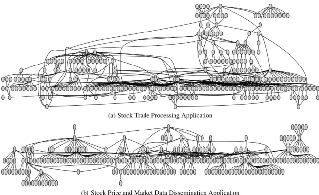
Today online server applications have become popular in do-mains ranging from banking, finance, e-commerce, and social net-working. Such server applications run on data centers and tend to be complex distributed systems with tens or hundreds of interact-ing software components runninteract-ing on large server clusters. As an example, consider an online stock trade processing application of a major financial firm, depicted in Figure 1(a). The application con-sists of 471 separate software components that process incoming
Permission to make digital or hard copies of all or part of this work for personal or classroom use is granted without fee provided that copies are not made or distributed for profit or commercial advantage and that copies bear this notice and the full citation on the first page. To copy otherwise, to republish, to post on servers or to redistribute to lists, requires prior specific permission and/or a fee.
Copyright 20XX ACM X-XXXXX-XX-X/XX/XX ...$10.00.
stock trades at low latencies; the graph depicts the flow of requests through the various application components. Figure 1(b) shows an-other application which disseminates stock prices and market news to the terminals of stock traders; this application consists of 8970 components. The components are depicted as nodes of the graph and process stock data and news from a multitude of sources, fil-ter, aggregate, and then disseminate updates for each company to desktops that subscribe to such streams. Such data center applica-tions differ significantly in scale and complexity when compared to traditional multi-tier web applications.
Typical data center applications evolve over time as new func-tionality is added, its workload volume grows, or its hardware or software is updated. To deal with such changes, an important man-agement task for administrators is to predict the impact of any planned (or hypothetical) change on the performance of individ-ual components or the entire system. This task, which is referred to aswhat-if analysis, requires the design of what-if models that take as input a potential change in the application workload or its settings and predict the impact of that change on application be-havior. However, given the complexity of today’s data center appli-cation, manual design of such what-if models is no longer feasible since data center administrators may not be able to comprehend the behavior of a complex system of tens of interacting components. Consequently, a what-if analysis system must be able to automat-ically derive such models from prior observations of application’s behavior. Further, the system must be able to scale to large com-plex applications with hundreds of interacting components, while allowing rich what-if analysis efficiently. While a number of mod-eling techniques have been proposed for distributed or multi-tier web applications [10, 14, 16, 13, 6, 12], such models are not di-rectly targeted for what-if analysis or are not designed to scale to larger data center applications such as the ones illustrated in Fig-ure 1.
In this paper, we present Predico, a what-if analysis system to predict the impact of workload changes on the behavior of data center applications. Predico makes the following contributions:
• Modeling of complex data center applications:Predico em-ploys a queuing-theoretic framework to model large distributed data-center applications. Our modeling framework is based on a network of queues and captures the dependence be-tween the workload of each component of the application and the corresponding resource utilization, request latency and the outgoing workloads to other components. Predico uses monitoring data and request logs to estimate the pa-rameters of such a model and employs model composition to create larger system-level models for groups of interacting
(a) Stock Trade Processing Application
(b) Stock Price and Market Data Dissemination Application
Figure 1: Structure of two production financial applications; only a subset of each application is shown for brevity.
application components.
• Intelligent query executionPredico uses a novel change prop-agation algorithm that uses these models to execute a what-if query and determine the impact of a workload change on other components. This algorithm first computes an influ-ence graph to determine which application components are impacted by the specified what-if query and then uses a change propagation technique to propagate the specified workload change through each component in the influence graph. The change propagation algorithm can handle application com-ponents that saturate due to a workload increase, which en-hances query result accuracy.
• Prototype Implementation: We have implemented a type of our Predico what-if modeling framework. Our proto-type incorporates a What-If Query Language (WIFQL) that can be used by administrators to pose queries. Since our pro-totype needs to handle large data center applications with hundreds of interacting components, we implement several optimizations to scale the modeling framework to such large applications. Specifically Predico uses on-the-fly model con-struction and employs a cache of preciously constructed mod-els to reduce model computation overhead.
• Evaluation based on real traces and real-world synthetic ap-plications.We conduct an experimental evaluation of Predico using traces of two large production applications from a fi-nancial institution as well as realistic synthetic applications. Our experimental results validate the accuracy of Predico’s modeling framework in building build node-level resource usage, latency and workload models and illustrate Predico’s ability to enable accurate what-if analysis.
2.
BACKGROUND AND PROBLEM
FORMU-LATION
Our work assumes a large distributed application withN inter-acting components. We assume that the application is structured as a directed acyclic graph (DAG), where each vertex represents a software component and edges capture the interactions (i.e., flow of requests) between neighboring nodes. For simplicity, we assume that each component runs on a separate physical (or virtual) ma-chine.1We assume that the DAG has one or more source nodes, that serve as entry points for application requests and one or more sinks, that serve as exits. The flow and processing of requests through such applications is captured by the DAG structure and is best ex-plained with examples.
Figure 1 depicts the DAGs of two production financial applica-tions. The first application is a stock trade processing application at a major financial firm; the application consists of 471 nodes and 2073 edges, of which a subset are shown in the figure. New stock trade requests arrive at one of the source nodes and flow through the system and exit from the sink nodes as “results”. Each intermediate node performs some intermediate processing on the trade request and triggers additional requests at downstream nodes. Nodes may aggregate incoming stock trades or break down a large stock order into smaller requests at downstream nodes. Figure 1(b) shows the structure of a market data dissemination application that dissemi-nates stock prices and news updates for a company to trading ter-minals (“desktops”) of stock traders. In this case, news items arrive from a number of sources and stock prices are obtained from a va-riety of exchanges, and this information is processed, transformed, filtered and/or aggregated and disseminated to any desktop node that has subscribed to information for a particular company. This application has 8970 nodes and 22719 edges and must provide
up-1This assumption is easily relaxed and we employ it for simplicity
dates at low latency in order for stock traders to make trades based on the latest market news.
Thus, we assume that requests flow through the DAG, with inter-mediate processing at each node; a request may trigger multiple re-quests at one or more downstream child nodes, and each node may aggregate requests from upstream parents. As can be seen, such ap-plication are significantly larger and more complex than traditional multi-tier web applications.
We assume that the DAG structure for each application is known a priori (there are automated techniques to derive the DAG struc-ture by observing incoming and outgoing traffic at each node [7]). We assume that each node in the DAG is a black box—i.e., we can observe the incoming and outgoing request streams along its edges and the total node-level utilization but that we have no knowledge of the internals of the software component and how it processes each request. This is a reasonable assumption in practice since IT administrators typically do not have direct knowledge of the appli-cation logic inside a software component, requiring us to treat it as a black box. However, administrators have access to request logs that the application components may generate and can also track OS-level resource utilizations on each node.
We assume that there areRdifferent types of requests in the en-tire distributed application. Each node can receive different types of requests belonging to theRtypes and can in turn trigger one or more requests of one of theRtypes at downstream child nodes. Given our black box assumption, the precise dependence of what type of outputs are generated by what set of inputs is unknown (and must be learned automatically by correlating request logs at a parent and a child). Similarly, the precise processing demands im-posed by a set of requests and the request latencies/response times are unknown and must also be learned.
Assuming such a data center application, our first problem is to model each application component (i.e., node of the DAG) by capturing the dependence between the incoming workload mix and the request latency, resource utilization, and the outgoing work-load. Second, we need to use thesenode-levelmodels to create
system-levelmodels that capture the behavior of a group of inter-acting nodes. Third, given such system-level models, we wish to enable rich workload-based what-if analysis of the distributed ap-plication. Such an analysis should allow administrators to pose what-if queries to determine the impact of a workload change at a particular node(s) on some other node(s) of the system. A typ-ical what-if query is assumed to contain two parts: (i) the“if ”
part, which specifies the hypothetical workload change, and (ii) the
“what”part, which specifies the nodes where the impact of this change should be computed. For instance, a volume-based what-if query could ask “what is the impact of doubling the volume of re-quests seen by source nodeion the incoming workload and CPU utilization seen at some downstream nodej?” Similarly, what-if analysis could pose queries on the impact of a change in the work-load mix: “what is the impact of a change in the workwork-load mix from< λA, λB,· · · >to< λ0A, λ
0
B,· · · >at intermediate node
ion the disk utilization of a downstream nodej?” Queries could also be concerned with the impact on latency: “what is the impact of doubling the volume of typeBrequests at nodejon the latency of requests at nodei?" Queries could also pose general questions such as “will any node in the system saturate if the incoming work-load at all source nodes increase by 30%?”.
Thus, to design our what-if analysis system, we must address the following three problems: (i) how should we model the dependence between the incoming workload at a node and the request latency, node utilization and the outgoing workload to downstream nodes? (ii) how should we combine node-level models to create
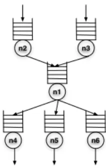
system-n1 n3 n2
n4 n5 n6
Figure 2: Modeling a data center application using an open network of queues
level models that capture the aggregate behavior of a group of in-teracting nodes in the DAG? (iii) what algorithms should be used to efficiently execute a what-if query using these models? From an implementation standpoint, we are interested in a fourth question as well: (iv) How should our system scale to complex data center applications with tens or hundreds of components?
3.
MODELING A DATA CENTER
APPLI-CATION
In this section, we first present a queuing model for a data cen-ter application that allows us to model the utilization and response time of these nodes. We then describe the construction of models to capture the input/output workload dependencies of these nodes. Finally, we explain how these node-level models are composed to construct system-wide models.
3.1
Queuing theoretic node-level models
Consider the DAG of a data center application withknodes de-noted byn1, . . . , nkandRdifferent type of requests. We model
the data center application using an open network ofkqueues, one for each node withRclasses of requests. We model each node as aM/G/1/P Squeue i.e. the service times are assumed to have an arbitrary distribution and the service discipline at each node is as-sumed to be processor sharing (PS). Requests can arrive at a queue from other queues which are its parents in the DAG or in the case of source nodes of the DAG from external sources. For analytical tractability we assume that the distribution of inter-arrival times of requests coming from outside have a poisson distribution. We de-note the arrival rates of requests of classrat the queueni from
outside byλr0,i. We assume that different classes of requests
ar-riving at a queue have different mean service rates. We denote the mean service rate of requests of classrat nodeibyµri.
Thus the DAG of a data center application is modeled as an open network of queues as shown in Figure 2. We use the well known queueing theory result called the BCMP theorem [3] to analyze this network of queues. The BCMP theorem states that for such queueing networks the utilization of a nodeni, denoted byρi, is
given by : ρi= R X i=1 ρri = R X i=1 λri µr i (1) whereρridenotes the resource utilization at nodenidue to class
rrequests,λri denotes the arrival rate of requests of typerat node
niand µri denotes the service rate of requests of typerat node
ni. This equation models the resource utilization of the node as
Similarly, the average number of requests of typerat nodeniunder
steady-state, denoted byKri, is given by:
Kri =
ρri
1−ρi
(2) We can now use Little’s Lawto find out the Tri, the average
response time of requests of typerat nodeniusing Equations 1
and 2: Tri = Kri λr i = 1 µr i(1−ρi) (3) This equation models the response time at a node as a function of the total node resource utilizationρiand the per-class service rate
µri.
Given a value for the per-class workload at a nodeλri we can
use Equation 1 to find out the utilizationρiand then use the
com-puted valueρito find out the response time using Equation 3. The
per-class service timesµir is the only unknown in the equations.
Since we assume that each node of the data center application is a black-box we need to estimate these unknowns from the available information gathered from monitoring of the node. We assume that requests logs at a node contain an entry for each incoming requests containing the timestamp and the requests string or type of request and that the resource utilization of the node is being periodically monitored using a tool likeiostat. Given such logs, multiple val-ues ofρi andλri can be collected over time. Since Equation 1
captures the relationship between theseR+ 1variables, the val-ues of the unknown per-class service ratesµri can be numerically
estimated using a regression method such as least squares.
3.2
Workload models
While queueing theory allows us to model the performance met-rics of a node, we also need to capture the relationship between the incoming workload and the outgoing workload of a node.
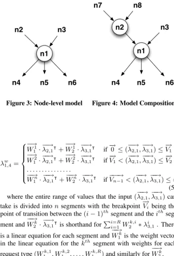
To understand the node-level workload models that Predico needs to build, consider the node shown in Figure 3. This noden1has
two parent nodesn2andn3and three child nodesn4, n5andn6.
Letλr2,1andλr3,1denote the arrival rate of requests of typerfrom
noden2andn3 respectively to noden1. Similarly, letλr1,4, λr1,5
andλr1,6denote the arrival rate of requests of typerat noden4, n5
andn6 respectively from noden1. Predico needs to build models
that capture the workload of each outgoing edge as functions of workload of the incoming edges. Thus, we seek a function for each ofλr1,4, λr1,5andλr1,6that expresses them as a function of
−−→
λ2,1and
−−→
λ3,1where
−→
λi,jis short-hand for observed rates of various request
types on the edge going from nodenitonji.e.(λi,j1 , λ2i,j,· · ·λRi,j)
. Similarly, we seek functions for each of the other request types :
λw1,4=f w 1,4( −−→ λ2,1, −−→ λ3,1) ,1≤w≤R (4)
We model workload-to-workload dependencies as piecewise lin-ear functions. Although these dependencies are linlin-ear in steady state, we choose piecewise linear modeling to capture various sys-tem artifacts like hot cache, cold cache and load-aware servers. Un-der this modeling assumption, we can rewrite Equation 4 as a set of linear functions : n1 n2 n3 n6 n5 n4
Figure 3: Node-level model
n1 n2 n3 n6 n5 n4 n7 n8
Figure 4: Model Composition
λw1,4= 8 > > > > < > > > > : −→ W11· −−→ λ2,1|+ −→ W21· −−→ λ3,1| if − → 0 ≤(−−→λ2,1, −−→ λ3,1)≤ − → V1 −→ W12· −−→ λ2,1|+ −→ W22· −−→ λ3,1| if − → V1<( −−→ λ2,1, −−→ λ3,1)≤ −→ V2 . . . . −−→ W1n· −−→ λ2,1|+ −−→ W2n· −−→ λ3,1| if −−−→ Vn−1<( −−→ λ2,1, −−→ λ3,1)≤ ∞ (5) where the entire range of values that the input(−−→λ2,1,
−−→
λ3,1)can
take is divided intonsegments with the breakpoint−→Vi being the
point of transition between the(i−1)thsegment and theith
seg-ment and−W−→2k· −−→ λ3,1|is shorthand forPii==1RW k,i 2 ∗λ i 3,1 . There
is a linear equation for each segment and−W−→k
1 is the weight vector
in the linear equation for thekthsegment with weights for each
request type(W1k,1, W
k,2 1 , . . . , W
k,R
1 )and similarly for
−−→
W2k.
Equation 5 relates the outgoing workload to incoming workload, but to use it for computing the outgoing workloadλw1,4for a given
value of incoming workload −−→λ2,1 and
−−→
λ3,1 we need to first find
the number of segments,n, and the breakpoints which define the segments, Vi,1 ≤ i ≤ n−1. We then need to find individual
linear functions for each segment by computing the weights of the corresponding linear functionW1kandW2k. We use a regression
analysis technique called multivariate adaptive regression splines ( MARS ) [4] that automatically fits piecewise linear functions on data. Predico uses the monitoring data that contains multiple mea-surements of the variables−−→λ2,1,
−−→
λ3,1 andλw1,4 to give as training
data to MARS which finds out the different segments and the linear function in each segment.
3.3
Model Composition: From Node-level to
System-level Models
Predico uses node-level models to construct system-wide models using model composition. Model composition essentially “chains” together multiple node-level models to compute the workload, re-source utilization and response time of a node as a function of one or more ancestor nodes. We illustrate the composition algorithm used by Predico using an example. Consider the sub-graph in Fig-ure 4 that shows a parent noden2, extending our earlier example
in Figure 3. At the node-level, Predico can compute the outgoing workload going from noden2to noden1,
−−→
λ2,1, as a set ofR
piece-wise linear functions, one for each request type : λw2,1=f w 2,1( −−→ λ8,2, −−→ λ7,2) ,1≤w≤R (6)
Equation 4 gives the outgoing workload going fron noden1ton4: λw1,4=f w 1,4( −−→ λ2,1, −−→ λ3,1) ,1≤w≤R (7)
Substituting the value of−−→λ2,1from Equation 6 into Equation 7 we
obtain a “composed model” : λw1,4=f w 1,4( −−→ f2,1( −−→ λ8,2, −−→ λ7,2), −−→ λ3,1) ,1≤w≤R (8) where−f−2→,1( −−→ λ8,2, −−→ λ7,2)is a shorthand for(f21,1( −−→ λ8,2, −−→ λ7,2), f22,1( −−→ λ8,2, −−→ λ7,2) , . . . , fR 2,1( −−→ λ8,2, −−→
λ7,2). Doing so enables the outgoing workload
sent from noden1 ton4 to be expressed as a function of
incom-ing workload of parent noden2. This process can be repeated for
the outgoing workload going to nodesn5andn6from noden1and
can also be recursively extended to nodes that are further upstream fromn2.
Creation of the composed model shown in Equation 8 requires composing the piecewise linear functionfw
1,4 with each of theR
piecewise linear functionsf2w,1,1 ≤ w ≤ R. Composing two
piecewise linear functionsf1andf2wheref1is defined by a set
ofL1segments with a linear function defined over each andf2is
defined by a set ofL2segments with a linear function defined over
each, can be performed inO(L1+L2)time by sorting the set of
breakpoints of bothf1andf2and then creating newL1+L2
seg-ments with a linear function defined over each segment where the linear function in each segment is obtained by simply composing the linear functions in the corresponding segments off1 andf2.
Thus the composed model shown in Equation 8 is again a piece-wise linear function which captures the relation between the out-going workload of noden1and the incoming workload of a parent
noden2.
We can now do a similar composition to find the dependence of the resource utilization of noden1, denoted byρ1, and the
re-sponse time of requests of typerat noden1, denoted byT
r
1on the
incoming workload of parent noden2denoted by
−−→
λ8,2,
−−→
λ7,2.
Sub-stituting Equation 6 into the resource utilization equation given by Equation 1 we get : ρ1 = R X i=1 ρi1= R X i=1 λi 1 µi 1 = R X i=1 λi3,1+λi2,1 µi 1 (9) = R X i=1 λi 3,1+f2i,1( −−→ λ8,2, −−→ λ7,2) µi 1 (10) which expresses the resource utilization of noden1as a function
of the incoming workload of noden2. Similarly, we can substitute
from Equation 10 into the response time Equation 3 to express the response time of request typer at noden1 as a function of the
incoming workload of parent noden2:
Tr1=
1 µr
1(1−ρ1)
(11)
4.
ANSWERING WHAT-IF QUERIES
In this section we describe the three step process used by Predico to answer a given what-if query. The execution of a what-if query is a three step process comprising of: 1) finding theinfluence graph
of the given query, 2) creating the node-level models of the nodes in theinfluence graphusing the modeling technique described above and 3) using thechange propagation algorithm to execute the query. We describe the three steps in greater detail below.
4.1
On-the-Fly Model Construction using the
Influence Graph
Since the number of nodes and edges in the DAG may be large in complex applications, it is not economical to precompute all possi-ble node-level models and periodically recompute models that have become invalid due to an actual workload or hardware change. In-stead Predico employs a “just-in-time” policy to compute models on-the-fly when a query arrives; only those models that are neces-sary to answer the query are computed. Models from prior queries are cached and reused if they are still valid. Predico uses the no-tion of aninfluence graphto determine which models should be constructed to answer a query. Given a what-if query, theinfluence graph is the set of all possible paths from the nodes in the “if ” part of the query to the nodes in the “what” part. Basically the influ-ence of a workload change will propagate along all paths from the “if” nodes/edges to the “what” nodes; so the influence graph cap-tures all of the nodes that must be considered to answer the query and other nodes in the DAG can be ignored.
Upon the arrival of a what-if query, Predico first computes the influence graph by generating the set of nodes that lie along all paths from the “if” nodes/edges to the “what” nodes. It then trig-gers on-demand construction of node-level workload models for all the nodes in the influence graph and node-level resource utilization and response time models for the “what” nodes alone. The use of the influence graph to prune the DAG and the reuse of previously computed models from the model cache enhances the scalability of the system and reduces computational overheads. The influence graph is also crucial for efficient query execution, as we will see in the next section.
4.2
Query Execution Using Change
Propaga-tion
Input : node-level models and influence graph for a what-if query
Output: value of workload/resource usage at "what" nodes/edges
forsIn"if" nodes/edgesdo
nodeQueue←s whilenodeQueue6=∅do currentNode←Pop(nodeQueue) foreInGetIncomingEdges(currentNode)do if ValueChanged(e)then GetChangedValue(e) else GetUnchangedValue(e) foroInGetOutgoingEdges(currentNode)do if ois in the influence graphthen
use node-level model ofcurrentNodeto find workload value ono
SetValue(o)
ValueChanged(o)=TRUE forcInGetChildNodes(currentNode)do
if cis in the influence graphthen
Push(nodeQueue,c)
Algorithm 1:Change Propagation via the Influence Graph
After creating the node-level models for the nodes of the influ-ence graph, Predico now needs to “execute” the query. Query exe-cution involves propagating the specified workload change through the influence graph, one node at a time, to compute its final im-pact on the nodes/edges specified in the “what” part of the query.
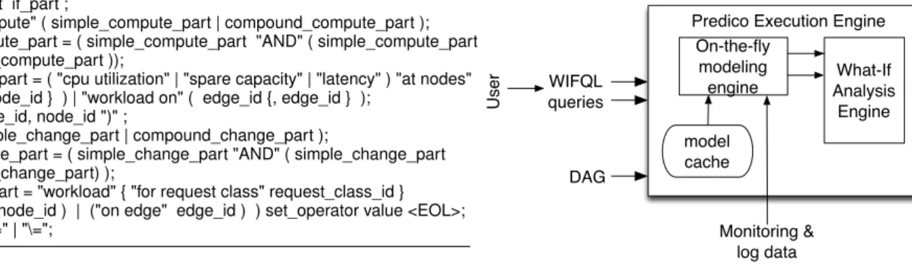
query = what_part if_part ;
what_part = "compute" ( simple_compute_part | compound_compute_part ); compound_compute_part = ( simple_compute_part "AND" ( simple_compute_part
| compound_compute_part ));
simple_compute_part = ( "cpu utilization" | "spare capacity" | "latency" ) "at nodes" node_id {, node_id } ) | "workload on" ( edge_id {, edge_id } );
edge_id = "(" node_id, node_id ")" ;
if_part = "if" ( simple_change_part | compound_change_part );
compound_change_part = ( simple_change_part "AND" ( simple_change_part | compound_change_part) );
simple_change_part = "workload" { "for request class" request_class_id } ( ("at node" node_id ) | ("on edge" edge_id ) ) set_operator value <EOL>; set_operator = "*=" | "\=";
Figure 5:The grammar for Predico’s What-If Query Language (WIFQL)
What-If Analysis Engine On-the-fly modeling engine model cache Monitoring & log data DAG WIFQL queries User
Predico Execution Engine
Figure 6: Predico Architecture
Once the workload change has been propagated to the nodes in the “what" part, the node-level models can be used to answer the query. Change propagation is equivalent to model composition— instead of directly computing a composed model for the “what” nodes/edges as a function of the “if” nodes/edges, the propagation algorithm propagates the specified change through the influence graph all the way down to the nodes/edges in the “what” part to achieve the same result.
Predico’s change propagation algorithm is described in Algo-rithm 1. Given node-level models and the influence graph, the change propagation algorithm traverses the influence graph in a breadth first manner. It starts with the nodes/edges in the “if” part and computes the values for the changed workload and then uses the model to compute its impact on the outgoing workload. This process is referred to as propagating the change from the incom-ing edges of a node to its outgoincom-ing edges. To illustrate, consider a query that is interested in estimating the impact of a doubling of the workload for a particular edge. If the original request rate was 10 req/s, then the new workload will be 20 req/s for that edge. This new value is used, along with theunchanged request ratesfor all other edges not impacted by the change, to compute the outgoing request rates for that node.
As shown in Figure 1, the algorithm proceeds in a breadth first fashion through the influence graph, starting with the “if” nodes/edges and computing the outgoing workload for each of the “if” nodes. The outgoing workload of a node becomes the incoming workload for downstream node(s), and the change propagation process re-peats, one node at a time, in a breadth-first fashion, until the change has propagated to all of the “what” nodes/edges. At this point, the algorithm computes the value of interest at the node by using the node-level models and terminates.
4.3
Saturation-aware Change Propagation
The basic change propagation algorithm outlined above naively assumes that each node has infinite resources and that any specified workload change will fully propagate through all of the nodes. In practice, however, each node has finite resources. If the change to the incoming workload causes the node to saturate, then only a portion of a workload increase will propagate to the downstream nodes and the remaining requests will be dropped. For example, if a node is presently servicing 100 req/s and is 70% utilized, then a doubling of the workload may cause the node to saturate long before the workload increases to 200 req/s and drop some of the incoming requests. Thus, downstream nodes will not see the full impact of the doubling of the workload at this parent node.
Hence change propagation must consider the impact of the work-load change on the node utilization and only propagate the full
workload change in the absence of saturation; otherwise, only that fraction of the workload increase, until saturation is reached, should be propagated. To do so, we enhance our basic change propagation algorithm to make it saturation-aware. Our enhanced algorithm also proceeds in a breadth-first fashion. However, it first com-putes the utilization of all resources on the node using the incoming workload rates (using Equation 1). If the utilization of any resource exceeds 100%, then the workload change will cause saturation on the node. In this case, the incoming request rates are reduced pro-portionately so that the utilization of the bottleneck resource drops to just under 100%. This reduced workload is propagated through the node, like before and the remaining requests are assumed to be dropped. On the other hand, if no resource utilization exceeds 100%, then the full incoming workload is propagated, like in the basic algorithm. Our enhanced algorithm ensures that the impact on the “what” nodes and edges will match the actual behavior in practice; a list of saturated intermediate nodes can be optionally listed with the query result.
5.
PREDICO IMPLEMENTATION
This section describes WIFQL, a query language that can be used to pose what-if queries to Predico and the implementation details of Predico prototype.
5.1
Posing What-if Queries in Predico
Since the goal of Predico is to enable users to understand the impact of potential workload changes on the system behavior, our system supports a simple query language to enable a rich set of queries to be posed by IT administrators. Any query in our What-If Query Language (WIFQL) has two parts: awhatpart and anif
part. Theif part of the query describes the hypothetical change, while thewhatpart asks the system to compute the impact of that change on different performance metrics at one or more nodes in the system. As an example of an WIFQL query, consider
compute workload on edges (n1,n4), (n1,n5) , (n1,n6) cpu utilization at nodes n1,n2 latency at nodes n1, n2
if workload on (n2,n1) *= 2 workload on (n3,n1) *= 0.5
This example query asks the system to compute the impact of a doubling of the workload along the edge going from noden2ton1
and a halving of the workload along the edge going from noden3
ton1 on the CPU utilization and latency at nodesn1 andn2and
the workload on the edges going from noden1to nodesn4,n5and
n6.
Figure 5 describes our query language grammar. As shown, the
work-load or changes to the hardware (e.g., a faster CPU). The workwork-load changes, which is the focus of this work, can be specified by iden-tifying one or more edges or nodes in the DAG and indicating a change in volume or a change in the mix of requests; set operators such as multiply and divide can be used to specify relative changes to the current workload, rather than absolute values. Thewhatpart specifies the performance metrics of interest at particular nodes or edges; several metrics are supported including resource utilizations, workloads, latencies or spare capacities. As indicated earlier, we assume that the DAG representing the application is known a priori and is used by queries to refer to particular nodes and edges of in-terest and specify workload changes on these nodes or edges.
5.2
Prototype Implementation
We have implemented a prototype of Predico using Python and the R statistical language to perform what-if analysis in large data center applications. Figure 6 depicts the high-level architecture of Predico.
The Predico frontend is implemented using a python implemen-tation of the lex and yacc parsing tools. It accepts user-posed queries and parses them by using the grammar rules of WIFQL. User-posed queries are then executed by the Predico execution engine, which comprises of two key components; the on-the-fly modeling engine and the what-if analysis engine. The on-the-fly modeling engine first computes the influence graph using a graph API in python and then creates node-level models by using on-the-fly model construc-tion. The modeling engine retrieves data about the workload on the incoming and outgoing edges of the node and the total resource utilization of the node and then invokes an R module for building the node-level models. The R module uses the MARS function present in the MDA package to build piecewise linear node-level workload models and the linear regression function to find the per-class service rates using least squares regression. Next, the what-if analysis engine uses these models to answer (“execute”) the query via the change propagation algorithm to propagate the hypotheti-cal workload change through the model and compute its impact on the nodes of interest to the user. The change propagation algorithm is again implemented by using the graph API written in python. The what-if analysis engine stores the node-level models computed by the modeling engine in a model cache that is implemented as three tables in the MySQL relational database engine; one each for storing the weight vectors used in node-level workload models, the breakpoints of the piecewise-linear model and the per-class service rates on a node required in the node-level resource utilization and response-time models.
6.
EXPERIMENTAL EVALUATION
In this section, we evaluate the performance of Predico by per-forming experiments on four applications. We first evaluate the ac-curacy of the analytical node-level resource utilization and response-time models and then the piecewise-linear workload models. We then perform experiments to ascertain the accuracy of system-level models formed by composition. We then employ Predico to per-form case studies where we pose what-if queries to Predico and compare the predictions with ground truth values observed in ac-tual experimental data.
6.1
Experimental Setup
We evaluate Predico on four different applications. These appli-cations are chosen from different domains and are of varying scale. The first two applications are from the financial domain and are
Application #Nodes #Edges Duration Metric # of Records Market Data 8970 22719 1 day outgoing bytes 7763764 Dissemintation
Stock Trade 471 2073 4 days outgoing requests 6060952 Processing
Table 1: Characteristics of Production Traces
being used by the data center of a financial institution. The third application is a benchmark e-commerce application. The fourth application is a synthetic Java enterprise application.
1. The topology of the first two applications, namely the stock trade processing and the market data dissemination applica-tion, is shown in Figure 1. We evaluate our system on traces collected from these two production financial applications. The traces collected from the stock trade processing applica-tion contain the total number of requests sent out by every component within every 30 second interval. The traces col-lected from the market data dissemination application con-tain data for the number of bytes sent out from every com-ponent on each of its outgoing edge, within every 30 second interval. Table 1 lists the characteristics of the traces. 2. The third application is the TPCW benchmark which models
an online bookstore application. We implement the TPC-W application as a 2-node Java servlet based application con-sisting of the front-end server (Tomcat) and a back-end database (MySQL). We use a testbed comprising of two virtual ma-chines for performing this experiment. Each virtual machine has a single 2.8 GHz Pentium 4 processor with 1GB memory. We use Tomcat version 5.5.26 and MySQL version 5.1.26 for setting up our TPC-W application. The TPC-W experi-mental setup allows us to monitor the end-to-end latency and resource utilization values apart from workload values. 3. The fourth application is an emulated application created from
several configurable Java servlets with each servlet running inside a Tomcat server that is itself running inside a virtual machine. The java servlet can be configured to take a desired processing time to process an incoming request and then trig-ger a desired number of requests to other such servlets. Thus, these servlets can be joined together in arbitrary ways to cre-ate large emulcre-ated data center applications having any de-sired topology.
6.2
Accuracy of Node-level Resource Usage and
Latency Models
We model the data center application as an open network of queues that lead to Equation 1 which captures the node-level re-source utilization and Equation 3 which captures the node-level la-tency. We validate the accuracy of this queueing model using the TPCW application running on a two server testbed.
The TPC-W web application exposes 14 different servlets which a customer visiting the website can invoke. We choose two of these servlets:“new products ”and“execute search”. We use thehttperf
load generation tool to simulate requests arriving from outside at the Tomcat server with exponentially distributed inter-arrival times.
Httperf allows us to generate workload for these servlets with dif-ferent arrival rates. The CPU utilization at the Tomcat server and the MySQL server are monitored every 1 second and the Tomcat logs contain an entry for each requests it processes and the end-to-end latency of each request. We vary the request arrival rate of the“execute search”servlet, denoted byλ10,1, from 100 to 200
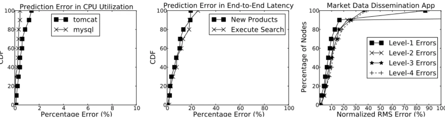
0 2
Percentage Error (%)
4 6 8 10 0 20 40 60 80 100CDF
Prediction Error in CPU Utilization
tomcat
mysql
Figure 7: Node-level Resource Usage model Accuracy 0 20
Percentage Error (%)
40 60 80 100 0 20 40 60 80 100CDF
Prediction Error in End-to-End Latency
New Products
Execute Search
Figure 8: Node-level Latency model Accu-racy 10 20 30 40 50 60 70 80 90 100
Normalized RMS Error (%)
0 20 40 60 80 100Percentage of Nodes
Market Data Dissemination App
Level-1 Errors
Level-2 Errors
Level-3 Errors
Level-4 Errors
Figure 9: Composed modeling for Market Data Dissemination App
requests per second with increases of 10 requests per second. Simi-larly we vary the request arrival rate of the“new products”servlet, denoted byλ20,1, from 10 to 100 requests per second with increase
of 10 requests per second. Thus we get 100 different pairs of re-quest arrival rates of each servlet. We run the system with each one of these 100 arrival rates for 15 minutes and monitor the CPU uti-lization and end-to-end latency. This gives us the average resource utilization at each nodeρ1, ρ2and the end-to-end latency for each
request type,T1 and T2. We use half of the 100 values for es-timating the values of the per-class service rates on each of the 2 nodes,µ1
1, µ21, µ12, µ22. We predict the per-node utilizationsρˆ1,ρˆ2
for the other 50 values using Equation 1. We use Equation 3 to pre-dict the per-node per-class response times,Tˆ11,
ˆ T21, ˆ T12, ˆ T22and add
the per-node response times to get the per-request-type end-to-end latenciesTˆ1andTˆ2. We find the prediction errors by comparing
the model predictions with the values seen during the experiment. Figure 7 and Figure 8 shows the distribution of prediction errors in terms of percentage relative error in predicting the resource utiliza-tion and latency respectively.
By using an open network of queue modeling, we are able to predict node-level CPU utilization to within 2% of the actual value. The median prediction error for response time using our modeling approach is less than 10%.We note that the accuracy of our model-ing approach is similar or better than recent techniques proposed in literature [9, 16, 12, 10] for modeling CPU utilization and re-sponse times .
6.3
Node-level Workload Models Accuracy
We evaluate the accuracy of using piecewise-linear functions created by using MARS to model the relationship of the outgoing workload of a node with the incoming workload of the node. We use the traces collected from the two applications to create these models and then ascertain the accuracy of these models.
For each of the two applications, we selected each component in turn and extracted the data for the workload on its incoming edges and outgoing edges. We then use MARS to estimate a function which expresses the workload on each outgoing edge of a node as a piecewise linear function of the workload on all the incoming edges on the node. We evaluate the accuracy of the piecewise lin-ear model in predicting the workload on each outgoing edge of this component. Cross-validation was used to measure the prediction accuracy; we divide the trace data for the selected component into training windows of 1 hour each and compute a model using MARS for each window for each outgoing edge. We then use each model to predict the data points outside of the window it was trained on;
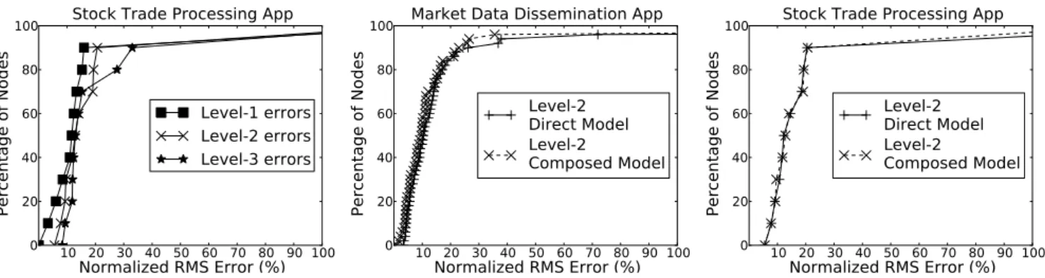
the deviations between the predicted and actual values were mea-sured. We use the root mean square (RMS) error as a metric of er-ror; we divide the RMS error by the range of actual values to report the results in normalized RMS error (%). The average normalized RMS error for the models of all the outgoing edges of a component is taken as the error for that component. We depict the errors for all the components of the two applications using CDF curves that show the percentage of components that have errors below a certain value. Figure 9 shows the errors for the market data dissemination application while Figure 10 shows the errors for the stock trade processing application. The curve labeled "Level-1" errors shows the CDF for the errors. We describe the concept of levels and the description about the "Level-2" and "Level-3" curves later in this section. The CDF curves indicate that the workload-to-workload models of 70% of the components have errors less than 10% in the case of the market data dissemination application while models for 80% of the components have errors less than 15% in the case of the stock trade processing application.
Our experimental results show that piecewise linear modeling provides accurate models of node-level workload for production data center applications.
6.4
Accuracy of System-level models with
in-creasing composition depth
We evaluate the accuracy of system-level models created by com-posing multiple level models. Composition of multiple node-level models leads to an accumulation of the error terms. We con-duct experiments to measure the increase in error with compos-ing increascompos-ing number of node-level models. We again use the traces from the two financial applications to evaluate the accuracy of system-level models. We reuse the node-level models of each component built for validating the accuracy of node-level workload models in the previous section for this experiment.
We select each component and compose its node-level workload model with that of its ancestor nodes to express the outgoing work-load of this component as a function of the incoming workwork-load of its ancestors. By using composition repeatedly we successively construct models expressing workload of a component as a function of its ancestors at different levels. Level 1 model is built between the outgoing workload of a component and its incoming workload. Level 2 model is built between the outgoing workload of a compo-nent and the incoming workload of its immediate parents. Similarly levelimodel is built between the component and its ancestors that are reachable in(i - 1)edges. We again use cross validation to com-pute the accuracy of these system-level models; we comcom-pute these models for each component using the trace data from one window
10 20 30 40 50 60 70 80 90 100
Normalized RMS Error (%)
0 20 40 60 80 100Percentage of Nodes
Stock Trade Processing App
Level-1 errors
Level-2 errors
Level-3 errors
Figure 10: Composed Modeling for Stock Trade Processing App
10 20 30 40 50 60 70 80 90 100
Normalized RMS Error (%)
0 20 40 60 80 100Percentage of Nodes
Market Data Dissemination App
Level-2
Direct Model
Level-2
Composed Model
Figure 11: Composed vs Direct Modeling for Market Data Dissemination App
10 20 30 40 50 60 70 80 90 100
Normalized RMS Error (%)
0 20 40 60 80 100Percentage of Nodes
Stock Trade Processing App
Level-2
Direct Model
Level-2
Composed Model
Figure 12: Composed vs Direct Modeling for Stock Trade Processing App
and use it to make predictions on the remaining windows. The aver-age normalized RMS error for the models of all the outgoing edges of a component is taken as the error for that component. Figures 9 and 10 show the CDF of normalized RMS errors for each level for the two applications. The CDF curve drops with increasing levels implying that the errors increase as we predict the workload of a node using ancestors higher up the node in the graph. Inspite of the increasing errors with increasing levels, the errors remain tolerable; for the Market Data Dissemination application even at level 4 the prediction errors for 80% of the nodes are less than 20%, while for the Stock Trade Processing at the level of 3 for 75% of the nodes the errors are less than 20%.
Composition of piecewise-linear node-level workload models yields system-level models which are also piecewise-linear. Instead of using composition repeatedly on multiple node-level models, we can also directly create system-level models that capture the rela-tionship between the incoming workload of a node and the work-load at some node downstream to this node. We can extract the data on the outgoing edges of the downstream node and the in-coming edges of the ancestor node and then use MARS to fit a piecewise-linear function just like in the case of creating a node-level workload model. We compare the CDF of errors obtained by using system-level models built using this direct modeling ap-proach with that obtained by using composition to build these mod-els. Figures 11 and 12 plot our results on traces of the Market Data Dissemination application and the Stock Trade Processing applica-tion respectively. The CDF of predicapplica-tion errors for models created using direct modeling closely follows the CDF of prediction errors obtained by using composition-based models. Composition based modeling, however, provides us with the added benefit of being able to reuse node-level models and can also account for node sat-uration, an aspect direct modeling can not capture.
Our results on using composition to create system-level models on the traces collected from the two production applications reveal that even with increasing composition depth, the system-level mod-els are effective in predicting workload.
6.5
Accuracy of System-level models with
vary-ing topology
The node-level models can be composed in a number of ways to create a system-level model depending on the topology of the DAG. We perform experiments to ascertain the prediction accuracy of composed models under different topologies. For this experiment we select some subgraphs in the DAGs for the two applications. We select subgraphs that correspond to three topologies-chain, split and join. These topologies correspond to different ways in which
e1 e2 e3 e4 e5 74 73 92 81 19 4 52 111 20 5 101
Prediction Source Prediction Target
e1 e2 e3 e4
e3 2.4% 2.6%
e4 4.7% 3.05% 4.39%
e5 4.67% 2.95% 4.33% 0.79%
(a) (b) (c)
Prediction Prediction Target
Source 81 19 74 73 4 92 111, 20, 5, 101, 52 12.47 % 12.45% 10.2% 9.28% 12.5 % 12.54% 19, 4, 92, 81 10.63% 9.46 % 74 3.34% (d)
Figure 13: Prediction Errors of composed modeling on differ-ent topologies
the components can interact with one another in an application: (i) in the chain topology, each component receives requests from a sin-gle upstream component, (ii) in the split topology, a component can send requests to multiple downstream components and (iii) in the join topology, a component can receive requests from multiple up-stream components. For each subgraph, we create node-level mod-els for each component and then use composition to create modmod-els to predict the workload on each outgoing edge of the subgraph. We measure prediction errors in predicting workload of each outgoing edge as a function of incoming workload of its ancestors at increas-ing levels.
Figures 13(a) and 13(b) show the subgraphs that we choose for this experiment. Figures 13(a) is from the Market Data Dissemi-nation application and Figure 13(b) is a subgraph from the Stock Trade Processing application. Figure 13(a) illustrates the chain and split topologies, while figure 13(b) is an example of a join topol-ogy. Tables 13(c) and 13(d) show how the errors of the composed models vary as we predict the workload on various edges/nodes of the graphs. For the subgraphs selected from the market data dis-semination application the prediction errors on all edges are within 5% while for the subgraph selected from the stock trade processing application the prediction errors are within 13%.
The errors reveal that Predico’s composition based modeling technique performs well even in case of complex application topolo-gies.
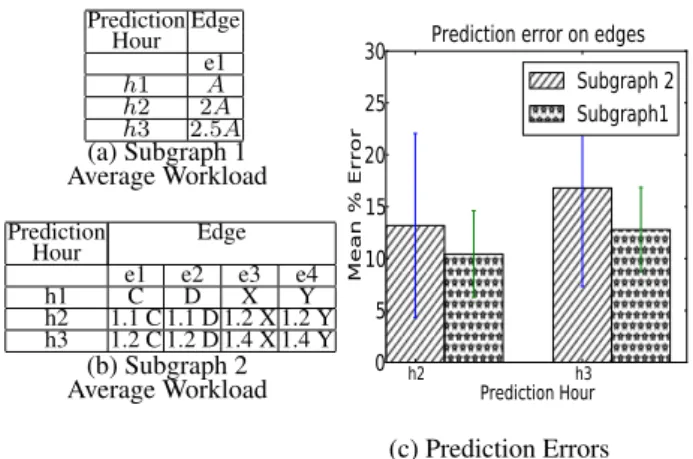
Prediction Edge Hour e1 h1 A h2 2A h3 2.5A (a) Subgraph 1 Average Workload Prediction Edge Hour e1 e2 e3 e4 h1 C D X Y h2 1.1 C 1.1 D 1.2 X 1.2 Y h3 1.2 C 1.2 D 1.4 X 1.4 Y (b) Subgraph 2
Average Workload h2
Prediction Hour
h30
5
10
15
20
25
30
Mean % ErrorPrediction error on edges
Subgraph 2
Subgraph1
(c) Prediction Errors
Figure 14: What-If case study on Market Data Dissemination Application
We create use-case scenarios to illustrate how Predico can be used in practice and evaluate its performance in answering what-if questions which commonly arise in large-scale applications. In this section, we pose workload-related what-if questions; we choose subgraphs from the market data dissemination application and the stock trade processing application and use Predico to predict the impact of workload changes on source nodes at the workload on the other edges of the subgraphs.
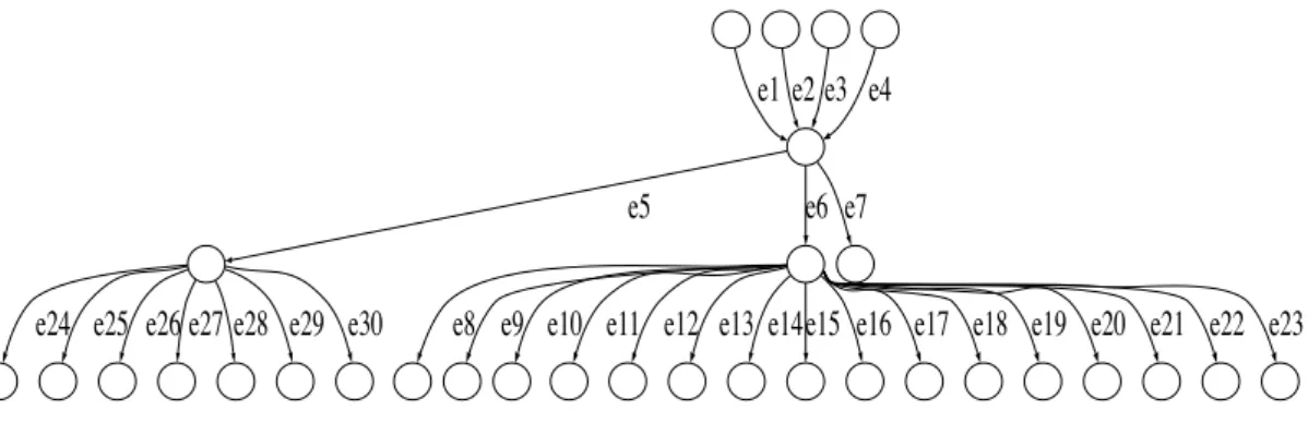
We first choose two subgraphs from the market data dissemina-tion applicadissemina-tion. The first subgraph has 1 source node while the other subgraph has 4 source nodes. Due to space constraint we show the topology of these subgraphs in Figure 17 and 18 in the Appendix.
On the first subgraph we pose the query: “what happens to the workload on downstream edges of subgraph 1 if the the outgoing workload of the single source node increases by 2 and 2.5 times the current value”. We examine the application traces and find periods of 1 hour duration each,h1,h2andh3, such that the outgoing
load from the source node increases by 2 and 2.5 times the work-load inh1in the hoursh2 andh3 respectively. Predico uses the
trace from hourh1and then predicts the workload values in hours
h2 andh3. We compare the ground truth value of the workload
seen in the two hours and compare Predico’s predictions to com-pute the errors. Figure 14(c) plots the average of the errors over all the downstream edges in terms of the normalized RMS error for each of the two changes mentioned in the what-if question.
The second subgraph has 4 source nodes and we pose a query which specifies different changes in workload on the 4 source nodes. We pose the query:“what happens to the workload on the down-stream edges of subgraph 2 if the outgoing workload at the source nodes changes to the values shown in Table 14(b)”. Again we em-ploy the same technique as we used in the previous experiment to find out Predico’s accuracy in answering this what-if query; we find out periods of 1 hour duration each in the application traces where these changes were observed and compare Predico’s predictions with ground truth values.
Figure 14(c) plots the average of the normalized RMS errors in predicting workload of all the edges of the two subgraphs for the 2 hours. The error bar charts show that Predico is able to answer what-if queries with less than 16% error for both these subgraphs.
We next choose two subgraphs from the stock trade processing application; subgraph 3 with 2 source nodes shown in Figure 15(a) and subgraph 4 with 3 source nodes shown in Figure 15(d).
On the first subgraph we pose the query: “what happens to the
workload on downstream edges of subgraph 3 if the workload on both the source nodes becomes 1.5 times and 3 times the current value”. We again compare Predico’s prediction with ground truth values observed in the traces to compute the errors. Similarly, on the second subgraph we pose a more complicated query where dif-ferent source nodes undergo difdif-ferent workload changes: “what happens to the workload on the downstream edges of subgraph 4 if the workload on the 3 source nodes changes to the values shown in Table 15(e)”. Figures 15(c) and 15(f) plot the normalized RMS error in predicting the outgoing workload for the other nodes of subgraph 3 and 4 respectively for the 2 hours for which predictions are made. For the subgraphs chosen from the stock trade processing application, Predico’s errors are less than 18%.
We hypothesize that some of the errors are due to idiosyncrasies of the trace. The trace collected from the stock trade processing ap-plication only contain the requests going out of each node and we assume that these requests are equally distributed among all its out-going edges; a possible cause of error. Similarly, in the case of the market data dissemination application, the traces contain the bytes sent out on each edge and we assume that the number of bytes are an approximation of the number of requests. This can again lead to errors since the same number of requests can lead to different bytes sent out. We note that even under these simplifying assumptions, Predico is able to make predictions with errors between 10% and 18%.
321
402 344
320 337
323
(a) Subgraph 3 PredictionNode Hour h1 A h2 1.5 A h3 3A (b) Subgraph 3Average Workload
h2
Prediction Hour
h3
0
2
4
6
8
10
12
14
16
18
% Error
Prediction error on nodes
Node 337
Node 344
Node 320
Node 402
(c) Subgraph 3 Prediction Errors 143 34 235 206 19 92 (d) Subgraph 4 Prediction Node Hour 143 19,92 h1 A B h2 1.12 A 1.5 B h3 1.8 A 1.65 B (e) Subgraph 4 Average Workloadh2
h3
Prediction Hour
0
2
4
6
8
10
12
14
16
18
% Error
Prediction error on nodes
Node 34
Node 235
Node 206
(f) Subgraph 4 Prediction Errors
Figure 15: What-if case study on Stock Trade Processing Ap-plication
6.7
Resource Usage What-if Analysis Case Study
on an emulated application where we pose resource-usage what-if questions. We construct this application using the configurable Java servlets described earlier.
Figure 16(a) shows the topology of the emulated application used for this experiment. We configure the nodes to send a desired num-ber of requests to downstream nodes and take a desired processing time for each request. Node 55 splits the requests it receives equally between node 52 and node 56. Each of these nodes then send the requests to node 54. Each request on node 56 takes 8 times the processing time it takes on node 55 while each request on node 52 takes half the processing time it takes on node 55. Each request on node 54 takes the same processing time as on node 55. The sys-tem is first run for half an hour each with incoming request rates of 10, 20 and 30 requests per second at node 55. Predico is given the monitoring data collected during this training phase and then we pose 2 what-if queries on Predico: “what is the CPU utiliza-tion at the nodes if the incoming workload at the source node is increased to 2 times and 3 times the current value”. During the test phase, we run the emulated application with incoming request rates of 40 requests per second and 60 requests per second for half an hour each to find the ground truth values of CPU utilization on all nodes. Table 16(b) shows the CPU utilization at all the nodes of the application observed during the training phase and test phase. As the table shows, CPU utilization reaches 100% at node 56 after the request rate reaches 40 requests per second.
Tables 16(c) shows the errors in terms of relative percentage er-rors in Predico’s answers obtained by using the basic propagation algorithm and the saturation-aware propagation algorithm. Since the errors for the two propagation techniques are the same for node 55 and node 52 we do not show them in the table. The errors reveal that saturation-unaware propagation makes errors in estimating the CPU utilization of node 56 and node 54. While for a 2x increase in workload, the saturation-unaware algorithm makes an error of 2.07% on node 56 and 17% on downstream node 54, its errors increase to 53% and 29% for the same nodes for the 3x increase what-if query. For a 3x increase in workload the saturation-unware propagation technique does not consider that node 56 has saturated and assumes that the entire workload continues to flows to down-stream node 54, leading to prediction errors. The saturation-aware propagation algorithm, however, is able to take into account node saturation and gives errors of 0.3% and 6% for both the what-if queries.
The results of this experiment with an emulated application show that Predico is able to predict resource utilization of nodes with high accuracy. Moreover, Predico’s change propagation algorithm is also able to take into account intermediate nodes saturating be-cause of excessive workload.
7.
RELATED WORK
A number of recent efforts have focused on building systems for performing what-if analysis on various distributed systems. The de-sign and implementation of a self-predicting cluster-based storage system is presented in [13]. The self-predicting system is able to answer what-if questions that administrators frequently ask about the impact of a decision on the performance of the system. The approach, however, involves intrusive instrumentation of the sys-tem in order to make it self-predicting. WISE [12] is a syssys-tem for answering what-if deployment and configuration questions for content distribution networks (CDN). This system enables the user to ask questions about the impact of commonly occurring CND scenarios like change in the mapping of clients to servers or de-ployment of a new data center. WISE deals with systems that span across large geographies and models the network latency part but
55 X 56 X/2 52 X/2 54 X/2 X/2
Workload CPU Utilization Node 55 Node 56 Node 52 Node 54 10 7.61872 25.8001 0.5521 5.26423 20 15.2392 51.6336 1.33517 10.9565 30 22.3839 76.4771 1.90553 17.4592 40 29.173199.18683.03971 27.8751 60 36.644899.55034.48884 27.0116 (b) Observed CPU Utilization
Query Saturation-Unaware Saturation-Aware Node 56 Node 54 Node 56 Node 54
2X increase 2.07 17 0.3 6.7
3X increase 53 29 0.4 6
(c) CPU Utilization Prediction Errors (%) (a) Topology
Figure 16: Resource Utilization What-If Analysis Case-Study
does not consider the server processing within data centers. Apart from systems that are directly aimed at performing what-if analysis, a number of modeling techniques have been proposed that predict the performance of the system under various workload conditions. These can be employed for answering what-if ques-tions about the system. A modeling approach for multi-tier internet applications based on queuing networks is proposed in [15]; mod-els are used to predict the response time of the application and the resource utilization at each tier under a given workload. Linear re-gression is used to predict the response time and throughput of the entire system in [16]. The modeling approach uses linear regres-sion to find out the service time of each transaction type and then uses queuing models to predict response time and throughput. An approach for automatically extracting all the invariants of the sys-tem and capturing them using models is proposed in [6] . Similar to our automatic model derivation, while the authors of this work also automatically derive node-level models, their technique is based on linear models while we have used a queuing-network model-ing based approach. All these techniques [15],[16],[6] are aimed towards multi-tier applications while Predico is targeted towards large-scale distributed systems. Nonstationarity in workloads is uti-lized to derive models for predicting the resource utilization and re-sponse time of an application as a function of workload volume and workload mix [10]. The technique is evaluated on production traces but the application used for evaluations has few servers. We eval-uate Predico on a much larger distributed system with hundreds of components and thousands of interactions. The modeling approach proposed in [11] creates "profiles" for the different components of a distributed application to model the resource demands placed by the components under different workloads on the underlying hard-ware. Using these models the system can predict the effect of work-load changes as well as hardware changes on the response time of the application; the technique is evaluated on benchmark ap-plications. IRONModel [14] proposes a modeling architecture for creating robust models. The models are used for answering what-if questions about the impact of reconfigurations on the response time and throughput of a large storage system. IRONModel, how-ever, involves intrusive instrumentation of the system for creating these models that is not a feasible solution in production environ-ments. Queueing models have also been used to model large scale systems [8]. The modeling framework automatically learns the pa-rameters of these queueing models by using a mathematical pro-gramming technique. The technique is validated by
experiment-ing with real world traces and predictexperiment-ing performance metrics like response times, end-to-end delays and utilization. We, in this pa-per, propose to automatically derive the required models to answer what-if questions. Building only the required models makes the technique scalable and enables incremental use of previously con-structed models.
A number of modeling techniques have also been used for per-formance debugging in distributed systems. A technique for au-tomatically inferring dependencies between the components of a large distributed application by only looking at the number of pack-ets exchanged between the difference components is proposed in [2]. These dependencies are then used to determine the source of a problem. Signal processing techniques have been used to au-tomatically discover causal paths in a distributed system by only utilizing passive measurements like the number of messages be-ing exchanged [1] . The technique discovers the delays bebe-ing en-countered at different nodes of the distributed application and this knowledge is used to ascertain paths that may be responsible for a large delay.
Similar to the WIFQL language provided by Predico to pose what-if questions, [5] also designed a new declarative language to enable administrators to find out the current performance of large scale applications and understand various performance correlations of the system.
8.
CONCLUSIONS
Data center operators often need to ascertain the impact of un-seen workload changes on large distributed applications. Predicting how a certain change in workload will influence complex data cen-ter applications is a challenging problem that needs automation. In this paper we presented Predico, a system which enables the user to perform "what-if" analysis on large distributed applications. Predico is non-intrusive and only uses commonly available moni-toring data to construct models and uses a new change propagation technique to estimate the impact of specified workload changes.
We modeled a large-scale data center application as an open net-work of queues to derive resource utilization, latency and net-workload models. We used traces from two large production applications from data centers of a major financial institution and data from syn-thetic enterprise applications to evaluate the efficacy of Predico’s what-if modeling framework. Our experimental evaluation vali-dated the accuracy of the node-level resource utilization, response time and workload models and then showed how Predico enables what-if analysis in four different applications.
9.
REFERENCES
[1] M. K. Aguilera, J. C. Mogul, J. L. Wiener, P. Reynolds, and A. Muthitacharoen. Performance debugging for distributed systems of black boxes. InSOSP ’03: Proceedings of the nineteenth ACM symposium on Operating systems principles, pages 74–89, New York, NY, USA, 2003. ACM Press. [2] P. Bahl, R. Chandra, A. Greenberg, S. Kandula, D. A. Maltz, and M. Zhang.
Towards highly reliable enterprise network services via inference of multi-level dependencies.SIGCOMM Comput. Commun. Rev., 37(4):13–24, 2007. [3] F. Baskett, K. M. Chandy, R. R. Muntz, and F. G. Palacios. Open, closed, and
mixed networks of queues with different classes of customers.J. ACM, 22(2):248–260, 1975.
[4] J. H. Friedman. Multivariate adaptive regression splines.The Annals of Statistics, 19(1):pp. 1–67, 1991.
[5] S. Ghanbari, G. Soundararajan, and C. Amza. A query language and runtime tool for evaluating behavior of multi-tier servers. InProceedings of the ACM SIGMETRICS international conference on Measurement and modeling of computer systems, SIGMETRICS ’10, pages 131–142, New York, NY, USA, 2010. ACM.
[6] G. Jiang, H. Chen, and K. Yoshihira. Discovering Likely Invariants of Distributed Transaction Systems for Autonomic System Management. InProc. of IEEE International Conference on Autonomic Computing (ICAC), pages 199–208, Dublin, Ireland, June 2006.
[7] A. Kind, P. Hurley, and J. Massar. A light-weight and scalable network profiling system.ERCIM News, 60, 2005.
[8] Z. Liu, L. Wynter, C. H. Xia, and F. Zhang. Parameter inference of queueing models for it systems using end-to-end measurements.Perform. Eval., 63(1):36–60, 2006.
[9] A. B. Sharma, R. Bhagwan, M. Choudhury, L. Golubchik, R. Govindan, and G. M. Voelker. Automatic request categorization in internet services.
SIGMETRICS Perform. Eval. Rev., 36(2):16–25, 2008.
[10] C. Stewart, T. Kelly, and A. Zhang. Exploiting nonstationarity for performance prediction. InEuroSys ’07: Proceedings of the 2nd ACM SIGOPS/EuroSys European Conference on Computer Systems 2007, pages 31–44, New York, NY, USA, 2007. ACM.
[11] C. Stewart and K. Shen. Performance Modeling and System Management for Multi-component Online Services. InProc. USENIX Symp. on Networked Systems Design and Implementation (NSDI), May 2005.
[12] M. Tariq, A. Zeitoun, V. Valancius, N. Feamster, and M. Ammar. Answering what-if deployment and configuration questions with wise.SIGCOMM Comput. Commun. Rev., 38(4):99–110, 2008.
[13] E. Thereska, M. Abd-El-Malek, J. J. Wylie, D. Narayanan, and G. R. Ganger. Informed data distribution selection in a self-predicting storage system. In
ICAC ’06: Proceedings of the 2006 IEEE International Conference on Autonomic Computing, pages 187–198, Washington, DC, USA, 2006. IEEE Computer Society.
[14] E. Thereska and G. R. Ganger. Ironmodel: robust performance models in the wild.SIGMETRICS Perform. Eval. Rev., 36(1):253–264, 2008.
[15] B. Urgaonkar, G. Pacifici, P. Shenoy, M. Spreitzer, and A. Tantawi. An Analytical Model for Multi-tier Internet Services and Its Applications. InProc. of the ACM SIGMETRICS Conf., Banff, Canada, June 2005.
[16] Q. Zhang, L. Cherkasova, and E. Smirni. A regression-based analytic model for dynamic resource provisioning of multi-tier applications. InICAC ’07: Proceedings of the Fourth International Conference on Autonomic Computing, Washington, DC, USA, 2007.
APPENDIX
Figures 17 and 18 show the two subgraphs of market data dissem-ination application which were chosen for the what-if analysis case study in Section 6.6. The subgraph in Figure 17 has 6 nodes with a single source node, while the larger subgraph shown in Figure 18 has 31 nodes and 4 source nodes.
e1
e2 e3 e4
e5
Figure 17: Subgraph 1 from the market data dissemination ap-plication
e1
e5
e6 e7
e2 e3 e4
e24 e25 e26 e27 e28 e29 e30
e8 e9 e10 e11 e12 e13 e14e15 e16 e17 e18 e19 e20 e21 e22 e23
Figure 18: Subgraph 2 from the market data dissemination ap-plication