A Generalized Inflated Poisson Distribution

(1)

A GENERALIZED INFLATED POISSON DISTRIBUTION

A thesis submitted to the Graduate College of

Marshall University In partial fulfillment of the requirements for the degree of

Master of Arts in Mathematics by Patrick Stewart Approved by

Dr. Avishek Mallick, Committee Chairperson Dr. Laura Adkins

Dr. Alfred Akinsete

Marshall University May 2014

(2)

ACKNOWLEDGEMENTS

I would like thank my thesis advisor, Dr. Avishek Mallick. He has helped me in numerous ways by giving me his advice, support, and guidance throughout the entire project. He has also assisted me by writing numerous recommendation letters and by challenging me in his classes.

I would also like to thank the other members of my thesis committee: Dr. Laura Adkins and Dr. Alfred Akinsete. Dr. Akinsete was always available to help me and to offer advice and is the most-wonderful chair of the math department. Dr. Laura Adkins is a wonderful professor who is always willing to help and answer questions that I may have.

Two other professors that I would like to thank are Dr. Gerald Rubin and Dr. Scott Sarra. Dr. Rubin is the professor who has challenged me the most and pushed me the hardest. I have learned so much from his classes, and I feel that he has thoroughly prepared me for a doctoral program. Also, his constant help, support, and advice on various situations are greatly appreciated. He is the professor who has made the largest impression on me throughout my time at Marshall University. Dr. Sarra is a professor who also has challenged me with his classes. Also, his wonderful help and support as my teaching mentor helped me through my teaching experience. I also appreciate both of these professors for their help in writing recommendation letters for me.

Dr. Carl Mummert also deserves my gratitude for being a constant source of help. He has helped me in numerous ways, and without his help I would not have made it through these past two years.

I would also like to thank my family for their support and help throughout all stages of my life. I would not have made it this far without them. Above all, glory to God for all things!

(3)

LIST OF FIGURES

3.1 Plots of the absolute SBias and SMSE of the MMEs and MLEs of π1 and λ (from

ZIP distribution) . . . 10 3.2 Plots of the absolute SBias and SMSE of the MMEs and MLEs ofπ1,π2 andλ(from

ZTIP distribution) . . . 12 3.3 Plots of the absolute SBias and SMSE of the MMEs and MLEs ofπ1,π2 andλ(from

ZTIP distribution) . . . 14 3.4 Plots of the absolute SBias and SMSE of the MMEs and MLEs ofπ1,π2, π3 and λ

(from ZOTIP distribution) . . . 15 3.5 Plots of the absolute SBias and SMSE of the MMEs and MLEs ofπ1,π2, π3 and λ

(from ZOTIP distribution) . . . 16 3.6 Plots of the absolute SBias and SMSE of the MMEs and MLEs ofπ1,π2, π3 and λ

(from ZOTIP distribution) . . . 17

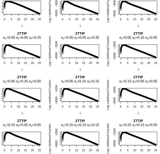
4.1 The graphs of the Log-Likelihood Function of a Zero-Two-Three Inflated Poisson

with varying values of π1,π2, and π3. . . 20

4.2 The graph of the observed frequencies compared to the estimated frequencies for the Zero-Two-Three Inflated Poisson. . . 24

(5)

LIST OF TABLES

1.1 Observed frequency of number of children (= count) per woman . . . 3 4.1 Results of several Inflated-Poisson Models after running MLE and χ2 Goodness of

(6)

ABSTRACT

Count data with excess number of zeros, ones or twos are commonly encountered in experimental situations. In this thesis we have examined one such fertility data from Sweden. The standard Poisson distribution, which is widely used to model such count data, may not provide a good fit to model women’s fertility (defined as the number of children per woman in her lifetime) in a specific population due to various cultural and sociological reasons. Therefore, the usual Poisson distribution is inflated at specific values suitably, as dictated by the societal norms, to fit the available data. The data set is examined using various tests and techniques to determine the validity of using a multi-point inflated Poisson distribution as compared to the standard Poisson distribution.

The various tests and techniques used include comparing the method of moment estimator of various multi-point inflated Poisson distributions along with the standard Poisson distribution. The maximum-likelihood estimators for Poisson distributions are also found and compared. Using simulation study, the maximum-likelihood and method of moment estimators were compared, and the maximum-likelihood estimator was found to have an overall better performance.

Validation for the results found involves using the Chi-square goodness of fit test on the various Poisson distributions. Another validation test involves comparing the Akaike information criterion (AIC) and the Bayesian information criterion (BIC) of the various Poisson distributions. The results of the various tests and techniques demonstrate that a multi-point inflated Poisson distribution provides a better fit and model as compared to the standard Poisson distribution.

Keywords and Phrases: Maximum-likelihood estimation, Method of moment estimator, Chi-square Goodness of fit test.

(7)

CHAPTER 1 INTRODUCTION

The widely used Poisson distribution of a discrete random variable that stands for the number or count of statistically independent events occurring within a unit time or space has the probability mass function (pmf) given as

p(k|λ) =P(X=k) =λkexp(−λ)/k! (1.1)

where k= 0,1,2, ....; and λ >0. Apart from its property as a limiting distribution of a binomial distribution, one can find many other characterizations in Feller (1968, 1971) [3] [4]. The list of applications of the Poisson distribution is quite varied and long as indicated by some of the references below:

• The number of soldiers of the Prussian army killed accidentally by horse-kick per year (von Bortkiewicz(1898) [9]);

• The number of bankruptcies that are filed in a month (Jaggia and Kelly (2012)[5]);

• The number of arrivals at a car wash in one hour (Anderson et al. (2012)[1]);

• The number of network failures per day (Levine et al. (2011) [6]);

• The number of blemishes per sheet of white bond paper (Doane and Seward (2010)[2]);

• The number of a particular type of insect that can be found in a 1-square-foot farmland (Pelosi and Sandifer (2003)[8]);

• The number of births, deaths, marriages, divorces, suicides and homicides over a given period of time (Weiers (2008)[10]).

Note that the Poisson model in (1.1), henceforth known as “Poisson(λ),” has both mean and variance = λ, which can pose problems in some applications where variation may differ from the

(8)

or overestimates the observed dispersion. This happens because the single parameterλ, over which the Poisson distribution is dependent, is often insufficient to describe the true observed distribution. In fact, in many cases, it is suspected that the overdispersion in the observed data is caused by population heterogeneity which goes unnoticed. This population heterogeneity is unobserved, in other words, the population consists of several subpopulations, but the subpopulation membership is not observed in the sample. A special form of heterogeneity is described by a ‘two-mass distri-bution’ giving mass π to count 0, and mass (1−π) to the second class which follows Poisson(λ). The result of this ‘two-mass distribution’ is the so called ‘Zero-Inflated Poisson distribution’ or ZIP distribution with the probability mass function

p(k|λ, π) =      π+ (1−π)e−λ ifk= 0 (1−π)p(k|λ) ifk= 0,1,2, .... (1.2)

whereλ >0, 0< π <1 andp(k|λ) is given in (1.1).

A further generalization of (1.2) can be obtained by inflating the Poisson distribution at several specific values. To be precise, if the discrete random variableX is thought to have inflated proba-bilities at the valuesk1, ...., km ∈ {0,1,2, ....}, then the following general probability mass function

can be considered: p(k|λ, πi,1≤i≤m) =      πi+ (1−Pm_i₌₁πi)p(k|λ) ifk=k1, k2...., km (1−Pm i=1πi)p(k|λ) ifk6=ki,1≤i≤m (1.3)

where k= 0,1,2, ....; λ >0, and πi ∈(0,1), 1≤i≤m, 0<Pm_i₌₁πi <1. For the remaining part

of this work, we will refer to (1.3) as the General Inflated Poisson (GIP) distribution which is the main focus of this work.

A special case of the GIP is the Zero-Two Inflated Poisson (ZTIP) obtained when usingk= 2, withk1 = 0 andk2= 2, which has been justified to model the Swedish women’s fertility dataset by

(9)

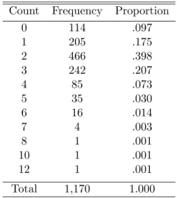
Count Frequency Proportion 0 114 .097 1 205 .175 2 466 .398 3 242 .207 4 85 .073 5 35 .030 6 16 .014 7 4 .003 8 1 .001 10 1 .001 12 1 .001 Total 1,170 1.000

Table 1.1: Observed frequency of number of children (= count) per woman

It has been suggested that the fertility of Swedish women tends to have higher counts of zeroes and twos. Zero children may be due to medical reasons or because some women might not have found the “right” man. On the other hand, a relative excess of twos may be explained by social processes, traditions of two-child family, and national institutional arrangements.

Whether a GIP with focus on (0,2) i.e., ZTIP (as argued by Melkersson and Rooth (2000) [7]) or a GIP with focus on (0,1,2) (called ’Zero-One-Two Inflated Poisson’ or ZOTIP) or some other set{k1, k2...., km}is appropriate for the above data will be eventually decided by a proper goodness

of fit test.

Therthraw moment ofXhaving a GIP (i.e., GIP(λ, πi,1≤i≤m;k1, ...., km)) can be obtained

from the following expression:

E(Xr) = m X i=1 kr_iπi+ (1− m X i=1 πi) ∞ X k=0 krp(k|λ) = m X i=1 kr_iπi+ (1− m X i=1 πi)µ 0 r. (1.4)

where µ0_r is the rth raw moment of Poisson(λ) which can easily be found from its moment generating function (MGF)exp{λ(exp(t)−1)}. Closed form expressions for the expectationE(X)

(10)

and varianceV ar(X) ofX for the ZTIP model can be obtained as

E(X) = 2π2+λ(1−π1−π2) (1.5)

V ar(X) = 4π2(1−π2) +λ(1−π1−π2){1 +λ(π1+π2)−4π2} (1.6)

In the next chapter, we first write the equations to obtain the method of moments estimators (MMEs) and then the maximum likelihood estimators (MLEs) of the parameters. In Chapter 3, we compare the performances of MMEs and MLEs for different GIP models using simulation studies. In Chapter 4, we revisit the dataset given in Table 1.1 and find the proper GIP model to fit the dataset.

(11)

CHAPTER 2

ESTIMATION OF GIP MODEL PARAMETERS

Given a random sample X1, ...., Xn, i.e. independent and identically distributed (iid) observations

from the GIP in (1.3) with parameters π1, ...., πm and λ, we first discuss the point estimation of

the parameters.

2.1 Method of Moments Estimation (MME)

The easiest way to obtain estimators of the parameters is through the method of moments estima-tion (MME). Assuming that the sample is a cross secestima-tion of the populaestima-tion, we equate the first (m + 1) sample moments with their population moments, i.e., we obtain a system of (m + 1) equations of the form m0_r= m X i=1 k_irπi+ (1− m X i=1 πi)µ 0 r(λ), r= 1,2, ....,(m+ 1); (2.1) wherem0_r=Pn

j=1Xjr/nis therthsample raw moments, andµ 0

r(λ) = (dr/dtr)exp{λ(exp(t)−1)}|t=0

is the rth raw moment of Poisson(λ). The values of πi, i= 1,2, ...., m, and λobtained by solving

the system of equations (2.1) are denoted by ˆπi(M M)and ˆλM M respectively. The subscript “(MM)”

indicates the MME approach. Note that all parameters are nonnegative, and hence all estimates also ought to be so. However, there is no guarantee that the corresponding MMEs of the parameters would obey this restriction. Hence, we propose ‘corrected MMEs’ as

ˆ

π(_i₍c_{M M}) ₎= ˆπi(M M) truncated at 0 and 1 and ˆλ (c) M M = ˆλ

∗

(2.2)

where ˆλ∗ is the solution ofλin (2.1) after substituting ˆπ(_i₍c_{M M}) ₎s. Later in Chapter 3, we will see in our simulation studies how to ensure that each ˆπ_i(₍c_{M M}) ₎ is between 0 and 1 as well as ˆλ(_{M M}c) >0.

In the special case of ZIP distribution, i.e., m = 1, k1 = 0, we have only two parameters: π1

and λ. The population mean and variance are, respectively,

(12)

By equating the above expressions with sample mean ( ¯X) and sample variances2 =Pn

j=1(Xj−

¯

X)2/(n−1) (which is an alternative approach instead of dealing withm0₁andm0₂), we get the MMEs ofπ1 andλas ˆπ1(M M) = (s2−X¯)/{X¯2+ (s2−X¯)}and ˆλM M = ¯X+ (s2/X¯)−1. Note that ˆπ1(M M)

becomes negative if ¯X > s2. Hence, our corrected MMEs are

ˆ π₁₍(c)_{M M}₎ =max{0,πˆ₁₍_{M M}₎}=      0 if ¯X > s2 ˆ π₁₍_{M M}₎ if ¯X ≤s2 (2.4) ˆ λ(₍c_{M M}) ₎=      ¯ X if ¯X > s2 ˆ λ₍_{M M}₎ if ¯X≤s2 (2.5)

In the above, ˆλ(₍c_{M M}) ₎ becomes ˆλ∗ = ¯X when ¯X > s2, i.e., ˆπ₁₍(c)_{M M}₎ = 0. This is the estimated value of λone obtains from (2.1) (for the special case of ZIP) after substituting ˆπ₁₍_{M M}₎ = 0.

In another special case of GIP, the Zero-Two Inflated Poisson (ZTIP) distribution, i.e., m = 2, k1 = 0, k2 = 2, we have three parameters: π1, π2 and λ. To obtain the MMEs of π1, π2 and λ

we equate the first three raw sample moments with their population counterparts. We obtain a system of three equations in three unknowns as follows:

2π2+λ(1−π1−π2) = m 0 1 4π2+λ(1 +λ)(1−π1−π2) = m 0 2 8π2+λ(1 + 3λ+λ2)(1−π1−π2) = m 0 3 (2.6)

In another special case of GIP, the Zero-One-Two Inflated Poisson (ZOTIP) distribution, i.e.,

m= 3, k1 = 0, k2 = 1, k3 = 2, we have four parameters: π1, π2, π3 and λ. To obtain the MMEs of

(13)

Thus we obtain a system of four equations in four unknowns as follows: π2+ 2π3+λ(1−π1−π2−π3) = m 0 1 π2+ 4π3+λ(1 +λ)(1−π1−π2−π3) = m 0 2 π2+ 8π3+λ(1 + 3λ+λ2)(1−π1−π2−π3) = m 0 3 π2+ 16π3+λ(1 + 7λ+ 6λ2+λ3)(1−π1−π2−π3) = m 0 4 (2.7)

Algebraic solutions to these systems of equations, ( i.e. the algebraic expressions for the MMEs of the parameters of interest) in (2.6) and (2.7) are obtained using Mathematica and are given in Appendix (B). We note that these solutions may not fall in the feasible regions of the parameter space, so we put restrictions to these solutions as discussed for the ZIP distribution to obtain the corrected MMEs.

2.2 Maximum Likelihood Estimation (MLE)

Another other approach of estimating parameters is the maximum likelihood estimation (MLE) method. Based on the data X = (X1, ...., Xn), the likelihood function L = L(λ, πi,1 ≤ i ≤

m;X) is defined as follows. Let Yi = number of observations at ki with inflated probability, i.e.,

Yi = Pnj=1I(Xj = ki),1 ≤ i ≤ m, where I is an indicator variable. Also, let Y. = Pmi=1Yi =

total number of observations with inflated probabilities, n = total number of observations, and (n−Y.) = total number of non-inflated observations. Then,

L= m Y i=1 {πi+ (1− m X l=1 πl)p(ki|λ)}Yi Y Xj6=ki {(1− m X l=1 πl)p(Xj|λ)} = m Y i=1 {πi+ (1− m X l=1 πl)p(ki|λ)}Yi(1− m X l=1 πl)(n−Y.) Y Xj6=ki p(Xj|λ) (2.8)

Thus, the loglikelihood function l∗ = lnL is

l∗= m X i=1 Yiln{πi+ (1− m X l=1 πl)p(ki|λ)}+ (n−Y.) ln(1− m X l=1 πl) + X Xj6=ki lnp(Xj|λ)

(14)

Since X Xj6=ki lnp(Xj|λ) =−λ(n−Y.) + lnλ( n X j=1 Xj− m X l=1 klYl) +c

wherec= (term free from the parameters), the loglikelihood function becomes

l∗= m X i=1 Yiln{πi+ (1− m X l=1 πl)p(ki|λ)}+ (n−Y.) ln(1− m X l=1 πl) −λ(n−Y.) + lnλ( n X j=1 Xj− m X l=1 klYl) +c (2.9)

The MLEs, ˆπiM L,1≤i≤m, and ˆλM L, are the values ofπi, 1≤i≤m, andλwhich maximizel∗

in (2.9) over the parameter space Θ ={(λ, π1, ..., πm)|0≤πi ≤1,1≤i≤m; 0≤Pmi=1πi ≤1, λ≥

0}. There are user-friendly softwares available which allow direct optimization of a multivariate function. But if maximization of l∗ is to be done by solving the system of equations, one can use the following traditional steps.

Taking partial derivatives of l∗ w.r.t. the parameters and setting them equal to zero yields

∂l ∂πi =Yi 1 {πi+ (1−Pml=1πl)p(ki|λ)} − m X t=1 Yt p(kt|λ) {πt+ (1−Pml=1πl)p(kt|λ)} − (n−Y.) (1−Pm l=1πl) = 0, ∀i= 1, . . . , m; ∂l ∂λ = m X i=1 Yi (1−Pm l=1πl)p(λ)(ki|λ) {πi+ (1−Pml=1πl)p(ki|λ)} −(n−Y.) +(nX¯ − Pm l=1klYl) λ = 0 (2.10) wherep(λ)(ki|λ) = (∂/∂λ)p(ki|λ) =p(ki−1|λ)−p(ki|λ), andp(−1|λ)≡0.

It is not clear whether the MME or the MLE provides overall better estimators. To the best of our knowledge, no comparative study has been reported in literature. Since the estimators do not have any general closed form expressions, simulation studies can provide some guidance about the performance of these two types of estimators. For this reason, we consider some special cases of the GIP withm= 1, 2 and 3 in the next chapter.

(15)

CHAPTER 3 SIMULATION STUDY

The following three cases are considered for our simulation study: (i) m= 1, k1 = 0 (Zero Inflated Poisson (ZIP) distribution)

(ii)m= 2, k1 = 0, k2 = 2 (Zero-Two Inflated Poisson (ZTIP) distribution)

(ii)m= 3, k1 = 0, k2 = 1, k3 = 2 (Zero-One-Two Inflated Poisson (ZOTIP) distribution)

For each special model mentioned above, we generate random data X1, ..., Xn from the

distri-bution (with given parameter values) N = 10000 times. Let us denote a parameter (either πi or

λ) by the generic notationθ. The parameterθ is estimated by two possible estimators ˆθ_{M M}(c) (the corrected MME) and ˆθM L (the MLE). At the lth replication, 1 ≤ l ≤ N, the estimates of θ are

ˆ

θ(_{M M}c)(l) and ˆθ_{M L}(l) respectively. Then the standardized bias (called ‘SBias’) and standardized mean squared error (called ‘SMSE’) are defined and approximated as

SBias(ˆθ) =E(ˆθ−θ)/θ≈ { N X l=1 (ˆθ(l)−θ)/θ}/N SMSE(ˆθ) =E(ˆθ−θ)2/θ2≈ { N X l=1 (ˆθ(l)−θ)2/θ2}/N (3.1)

Note that ˆθwill be replaced by ˆθ(_{M M}c) and ˆθM Lin our simulation study. Further observe that we

are using SBias and SMSE instead of the actual Bias and MSE, because the standardized versions are more informative. An error of magnitude 0.01 in estimating a parameter with true value 1.00 is more severe than a situation where the parameter’s true value is 10.0. This fact is revealed through SBias and/or SMSE than the actual bias and/or MSE.

3.1 The ZIP Distribution

In order to set the stage for the simulation study for the Zero Inflated Poisson (ZIP) distribution, we fix λ = 3 and vary π1 from 0.1 to 0.8 with an increment of 0.1 for n = 25. The constrained

optimization algorithm “L-BFGS-B” is implemented to obtain the maximum likelihood estimators (MLEs) of the parameters λand π , and the MMEs are obtained by solving a system of equations

(16)

and imposing appropriate restrictions on the parameters. In order to compare the performances of the MLEs with that of the MMEs, we plot the absolute standardized biases (SBias) and stan-dardized MSE (SMSE) of these estimators obtained over the allowable range ofπ1. The SBias and

SMSE plots are presented in Figure 3.1.

● ● ● ● ● ● 0.1 0.2 0.3 0.4 0.5 0.6 0.7 0.8 −0.10 0.00 0.10 0.20 (a) SBias ● ● ● ● ● ● 0.1 0.2 0.3 0.4 0.5 0.6 0.7 0.8 −0.4 0.0 0.2 0.4 (b) SBias ● ● ● ● _● ● 0.1 0.2 0.3 0.4 0.5 0.6 0.7 0.8 0.0 0.5 1.0 1.5 (c) SMSE ● ● ● ● ● ● 0.1 0.2 0.3 0.4 0.5 0.6 0.7 0.8 −0.1 0.1 0.3 0.5 (d) SMSE

Figure 3.1: Plots of the absolute SBias and SMSE of the MMEs and MLEs of π1 and λ(from ZIP

distribution) plotted againstπ1 forλ= 3 and n= 25. The solid line represents the absolute SBias

or SMSE of the corrected MME. The dashed line represents the absolute SBias or SMSE of the MLE. (a) Comparison of absolute SBias of π1 estimators. (b) Comparison of absolute SBias ofλ

(17)

MME with respect to SBias. However, MME outperforms the MLE from about 0.18 until around 0.35. From this point until about π1 = 0.6, MLE slightly outperforms the MME. After this point,

SBias of MME can no longer be calculated. The Sbias seems to be the smallest for MME at 0.2 and for MLE at around 0.4. In Figure 3.1(b), we see that MLE uniformly outperforms the MME until 0.6, after which again SBias of MME can no longer be calculated. They are both essentially unbiased since the SBias seems to be basically zero for MLE and around .01 or less for MME. In Figure 3.1(c), MLE consistently outperforms MME at all points until 0.6 where they both seem to have nearly the same SMSE. After 0.6, SMSE of MME cannot be calculated anymore. For both MLE and MME, the SMSE starts off at their highest values and then decreases rapidly until it reaches nearly zero. SMSE of MLE consistently outperforms that of MME in Figure 3.1(d). They both start off at their lowest values, and at this point, both MME and MLE has nearly the same SMSE. Again, SMSE of MME cannot be calculated after 0.6. It appears that SMSEs for both MME and MLE increase as values of π1 get higher.

So we see for the ZIP distribution, the MLEs of the parameters π1 and λperform better than

the MMEs almost everywhere over a certain range ofπ1, namely 0.1 - 0.6, when the sample size is

25. We note that MLEs of both parameters have smaller absolute SBias and SMSE as compared to those of MMEs.

3.2 The ZTIP Distribution

In the case of the Zero-Two Inflated Poisson (ZTIP) distribution we have three parameters to consider, namely π1,π2 and λ. For fixedλ= 3 we varyπ1 and π2 one at a time for sample size n

= 25. Figure 3.2 presents the six comparisons for ˆπ(₁₍c)_{M M}₎, ˆπ(₂₍c)_{M M}₎ and ˆλ(₍c_{M M}) ₎ with ˆπ1(M L), ˆπ2(M L)

and ˆλ(M L)in terms of absolute standardized bias and standardize MSE forn= 25, varyingπ1 from

0.1 to 0.4 and keeping π2 andλfixed at 0.15 and 3 respectively.

In Figure 3.2(a), MLE outperforms MME at all points with respect to absolute SBias. Both start above zero and decrease slightly until 0.2. Absolute SBias of MLE increases linearly until 0.3, but absolute SBias of MME stays same until this point. However, after 0.3 absolute SBias of both MME and MLE is increasing until the end. In Figure 3.2(b), we see that the MLE is essentially unbiased for all values ofπ1, and absolute SBias of MME vary a lot and is always more

(18)

● ● ● 0.10 0.15 0.20 0.25 0.30 0.35 0.40 −0.1 0.1 0.3 0.5 (a) SBias ● ● ● 0.10 0.15 0.20 0.25 0.30 0.35 0.40 −0.1 0.1 0.3 0.5 (b) SBias ● ● ● ● 0.10 0.15 0.20 0.25 0.30 0.35 0.40 −0.1 0.1 0.3 0.5 (c) SBias ● ● ● ● 0.10 0.15 0.20 0.25 0.30 0.35 0.40 0.2 0.6 (d) SMSE ● ● ● ● 0.10 0.15 0.20 0.25 0.30 0.35 0.40 0.5 1.0 1.5 2.0 (e) SMSE ● ● ● 0.10 0.15 0.20 0.25 0.30 0.35 0.40 0.02 0.08 0.14 (f) SMSE

Figure 3.2: Plots of the absolute SBias and SMSE of the MMEs and MLEs ofπ1,π2 and λ(from

ZTIP distribution) by varying π1 for fixed π2 = 0.15,λ= 3 and n= 25. The solid line represents

the absolute SBias or SMSE of the corrected MME. The dashed line represents the absolute SBias or SMSE of the MLE. (a)-(c) Comparisons of absolute SBiases ofπ1,π2andλestimators respectively.

(19)

than that of MLE. Thus for all permissible values of π1, MME performs more poorly than MLE,

except atπ1 = 0.2, where both are unbiased. Again in Figure 3.2(c), we see the same trend. MLE

is unbiased throughout and MME is performing very poorly. In Figure 3.2(d), MME starts of with a lower SMSE than MLE. Both intersect at about π1 = 0.15. After this point, MLE consistently

outperforms the MME with respect to MSE. Both decrease until about 0.3 before going up, but SMSE of MLE stays below that of MME. In Figures 3.2(e) and 3.2(f), SMSE of MLE stays constant at 0.6 and 0.04 respectively for all permissible values of π1. Also MME performs way worse for

both the cases.

In our second scenario which is presented in Figure 3.3, we varyπ2keepingπ1andλfixed at 0.15

and 3 respectively. In Figures 3.3(a) and 3.3(c), we see that MLE outperforms MME throughout with respect to absolute SBias. Moreover MLE is unbiased atπ2 = 0.2 in Figure 3.3(a) and almost

so at all values of π2 in Figure 3.3(c). However in Figure 3.3(b), absolute SBias of MME starts

off quite high, then it sharply decreases until π2 = 0.2. After that MME performs nearly as well

as the MLE. From Figures 3.3(d), 3.3(e) and 3.3(f), it is clear that MLE outperforms MME with respect to SMSE for all permissible values of π2. Thus we observe that the MLEs of the all three

parameters perform better than the MMEs in terms of the both absolute SBias and SMSE.

3.3 The ZOTIP Distribution

For the Zero-One-Two Inflated Poisson (ZOTIP) distribution we have four parameters to consider, namely π1, π2, π3 and λ. For fixed λ = 3 we vary π1, π2, and π3 one at a time for sample

size n = 25. Thus we have eight comparisons for ˆπ₁₍(c_{M M}) ₎, ˆπ₂₍(c)_{M M}₎, ˆπ(₃₍c)_{M M}₎ and ˆλ(₍c_{M M}) ₎ with ˆ

π1(M L), ˆπ2(M L), ˆπ3(M L) and ˆλ(M L). These comparisons in terms of absolute standardized bias and

standardize MSE are presented in Figures 3.4-3.6.

In the first scenario of ZOTIP distribution, which is presented in Figure 3.4, we varyπ1keeping

π2,π3 andλfixed at 0.2, 0.2 and 3 respectively. From Figure 3.4(a, b, c, d), we see that the MMEs

of all the four parameters perform consistently worse than the MLEs. Also, the MLEs seem to be unbiased for all permissible values of π1. Moreover absolute SBias as well as SMSE of MME of

λ become infinite (or cannot be calculated) after π1 = 0.2, which is evident from boxes (d) and

(20)

● ● ● ● 0.10 0.15 0.20 0.25 0.30 0.35 0.40 −0.2 0.2 0.6 1.0 (a) SBias ● ● ● ● 0.10 0.15 0.20 0.25 0.30 0.35 0.40 −0.2 0.2 0.6 1.0 (b) SBias ● ● ● ● 0.10 0.15 0.20 0.25 0.30 0.35 0.40 −0.2 0.2 0.6 1.0 (c) SBias _● ● ● ● 0.10 0.15 0.20 0.25 0.30 0.35 0.40 0.2 0.4 0.6 0.8 (d) SMSE ● ● ● _● 0.10 0.15 0.20 0.25 0.30 0.35 0.40 1 2 3 4 (e) SMSE ● ● _● ● 0.10 0.15 0.20 0.25 0.30 0.35 0.40 0.02 0.08 0.14 (f) SMSE

Figure 3.3: Plots of the absolute SBias and SMSE of the MMEs and MLEs ofπ1,π2 and λ(from

ZTIP distribution) by varying π2 for fixed π1 = 0.15,λ= 3 and n= 25. The solid line represents

the absolute SBias or SMSE of the corrected MME. The dashed line represents the absolute SBias or SMSE of the MLE. (a)-(c) Comparisons of absolute SBiases ofπ1,π2andλestimators respectively.

(21)

● ● ● ● ● 0.1 0.2 0.3 0.4 0.5 0.0 2.0 (a) SBias ● ● ● ● ● 0.1 0.2 0.3 0.4 0.5 0.0 2.0 (b) SBias ● ● ● ● ● 0.1 0.2 0.3 0.4 0.5 0.0 2.0 (c) SBias ● ● 0.1 0.2 0.3 0.4 0.5 0.0 2.0 (d) SBias ● ● ● _● ● 0.1 0.2 0.3 0.4 0.5 0 6 12 (e) SMSE ● ● ● ● ● 0.1 0.2 0.3 0.4 0.5 0.2 0.8 (f) SMSE ● ● ● ● ● 0.1 0.2 0.3 0.4 0.5 0 3 6 (g) SMSE ● ● 0.1 0.2 0.3 0.4 0.5 0.0 0.3 (h) SMSE

Figure 3.4: Plots of the absolute SBias and SMSE of the MMEs and MLEs of π1, π2, π3 and λ

(from ZOTIP distribution) by varyingπ1 for fixed π2 =π3 = 0.2 andλ= 3 and n= 25. The solid

line represents the absolute SBias or SMSE of the corrected MME. The dashed line represents the absolute SBias or SMSE of the MLE. (a)-(d) Comparisons of absolute SBiases of π1,π2,π3 andλ

(22)

parameters perform consistently worse than the MLEs. ● ● ● ● 0.10 0.15 0.20 0.25 0.30 0.35 0.40 0.0 2.0 (a) SBias ● ● ● ● 0.10 0.15 0.20 0.25 0.30 0.35 0.40 0.0 2.0 (b) SBias ● ● ● ● 0.10 0.15 0.20 0.25 0.30 0.35 0.40 0.0 2.0 (c) SBias ● ● 0.10 0.15 0.20 0.25 0.30 0.35 0.40 0.0 2.0 (d) SBias ● ● ● ● 0.10 0.15 0.20 0.25 0.30 0.35 0.40 0 2 4 (e) SMSE ● ● ● ● 0.10 0.15 0.20 0.25 0.30 0.35 0.40 0.0 1.0 2.0 (f) SMSE ● ● ● ● 0.10 0.15 0.20 0.25 0.30 0.35 0.40 0 3 6 (g) SMSE ● ● 0.10 0.15 0.20 0.25 0.30 0.35 0.40 0.0 1.0 2.0 (h) SMSE

estimators respectively. (e)-(h) Comparisons of SMSEs of π1,π2,π3 andλestimators respectively.

In our second scenario which is presented in Figure 3.5, we vary π2 keepingπ1,π3 and λfixed

(23)

● ● ● ● ● 0.1 0.2 0.3 0.4 0.5 −2 0 2 (a) SBias ● ● ● ● ● 0.1 0.2 0.3 0.4 0.5 −2 0 2 (b) SBias ● ● ● _● ● 0.1 0.2 0.3 0.4 0.5 −1 2 4 (c) SBias ● 0.1 0.2 0.3 0.4 0.5 −1 1 3 (d) SBias ● ● ● ● _● 0.1 0.2 0.3 0.4 0.5 −2 0 2 (e) SMSE ● ● ● ● ● 0.1 0.2 0.3 0.4 0.5 −2 0 2 (f) SMSE ● ● ● ● _● 0.1 0.2 0.3 0.4 0.5 0 10 20 (g) SMSE ● 0.1 0.2 0.3 0.4 0.5 −1.0 0.5 (h) SMSE

(24)

In the third scenario which is presented in Figure 3.6, we vary π3 keeping π1, π2 and λ fixed

at 0.2, 0.2 and 3 respectively. Here also we observe similar results as the first two cases of ZOTIP distribution, MLEs being unbiased for all the four parameters and uniformly outperforming MMEs. Also as before MLEs uniformly outperform MMEs of all the four parameters with respect to SMSE. SBias and SMSE of MME ofλbecome infinite just afterπ1 = 0.1 as such performs even worse than

both the previous cases.

Thus from our simulation study it is evident that MLE has an overall better performance than MME for all the GIP models. So in the next chapter, we consider an example where we fit an appropriate GIP model to a real life data set.

(25)

CHAPTER 4

AN APPLICATION OF GIP DISTRIBUTION

In this chapter, we revisit the Swedish fertility data presented in Table 1.1. The objective here is to fit a suitable GIP. Melkersson and Rooth [7] proposed a ZTIP model for the dataset. But, our analysis shows that perhaps a ZTTIP (‘Zero-Two-Three Inflated Poisson’) is more suitable. Since our simulation study points out that the MLE has an overall better performance, all of our estimations of model parameters are carried out using this approach. For the sake of completeness, we have also included the MMEs. The details of our model fitting is presented below.

For various values of π1, π2, and π3, we plotted the log-likelihood function of the ZTTIP for

λ, as presented in Figure 4.1. Figure 4.1 demonstrates that for each value of πi there exists one

global maximum for λ. Therefore, we can conclude that using the MLE is a justified approach for estimating for λ. The same procedures were also carried out for each πi, and in each case, there

exists only one global maximum for each parameter.

Table 1.1 shows significantly high frequencies at the values 0, 1, 2 and 3. Therefore, we tried all possible combinations of GIP models. First, we try with single-point inflation at each of these four values (i.e., 0, 1, 2 and 3). In this first phase, an inflation at 2 seems most plausible as it gives the highest p-value. Next, we try two-point inflations at{0, 1},{0, 2},{0, 3},{1, 2}, etc. At this stage, {2, 3} inflation seems the most appropriate going by both the p-value as well as AIC and BIC. This disproves the claim made by Melkersson and Rooth [7] that ZTIP, {0, 2}, is the best among the two-point inflated models. Table 4.1 gives the details from our model fitting. Table 4.1 includes all possible inflated Poisson models, chi-square goodness of fit test statistics, degrees of freedom (= number of categories in Table 1.1 - number of parameters in GIP model), p-values and AIC and BIC values. Note that the last three categories of Table 1.1 are collapsed into one due to small frequencies.

In the next stage, we try three-point inflation models, and here we note that a GIP with inflation set{0, 2, 3}significantly improves over the earlier{2, 3} inflation model (i.e., TTIP). This ZTTIP significantly improves the p-value while maintaining a low AIC and BIC. We fitted the full{0, 1,

(26)

ZTTIP ● ● ● ●●●●●●●●●●●●●●●●●●●●●●●●●●●●●●●●●●●●●●●●●●●●●●●●●●●●●●●●●●●●●●●●●●●●●●●●●●●●●●●●●●●●●●●●●●●●●●●●●●●●●●●●●●●●●●●●●●●●●●●●●●●●●●●●●●●●●●●●●●●●●●●●●●●●●●●●●●●●●●●●●●●●●●●●●●●●●●●●●●●●●●●●●●●●●●●●●●●●●●●●●●●●●●●●●●●●●●●●●●●●●●●●●●●●●●●●●●●●●●●●●●●●●●●●●●●●●●●●●●●●●●●●●●●●●●●●●●●●●●●●●●●●●●●●●●●●●●●●●●●●●●●●●●●●●●●●●●●●●●●●●●●●●●●●●●●●●●●●●●●●●●●●●●●●●●●●●●●●●●●●●●●●●●●●●●●●●●●●●●●●●●●●●●●●●●●●●●●●●●●●●●●●●●●●●●●●●●●●●●●●●●●●●●●●●●●●●●●●●●●●●●●●●●●●●●●●●●●●●●●●●●●●●●●●●●●●●●●●●●●●●●●●●●●●●●●●●●●●●●●●●●●●●●●●●●●●●●●●●●●●●●●●●●●●●●●●●●●●●●●●●●●●●●●●●●●●●●●●●●●●●●●●●●●●●●●●●●●●●●●●●●●●●●●●●●●●●●●●●●●●●●●●●●●●●●●●●●●●●●●●●●●●●●●●●●●●●●●●●●●●●●●●●●●●●●●●●●●●●●●●●●●●●●●●●●●●●●●●●●●●●●●●●●●●●●●●●●●●●●●●●●●●●●●●●●●●●●●●●●●●●●●●●●●●●●●●●●●●●●●●●●●●●●●●●●●●●●●●●●●●●●●●●●●●●●●●●●●●●●●●●●●●●●●●●●●●●●●●●●●●●●●●●●●●●●●●●●●●●●●●●●●●●●●●●●●●●●●●●●●●●●●●●●●●●●●●●●●●●●●●●●●●●●●●●●●●●●●●●●●●●●●●●●●●●●●●●●●●●●●●●●●●●●●●●●●●●●●●●●●●●●●●●●●●●●●●●●●●●●●●●●●●●●●●●●●●●●●●●●●●●●●●●●●●●●●●●●●●●●●●●●●●●●●●●●●●●●●●●●●●●●●●●●●●●●●●●●●●●●●●●●●●●●●●●●●●●●●●●●●●●●●●●●●●●●●●●●●●●●●●●●●●●●●●●●●●●●●●●●●●●●●●●●●●●●●●●●●●●●●●●●●●●●●●●●●●●●●●●●●●●●●●●●●●●●●●●●●●●●●●●●●●●●●●●●●●●●●●●●●●●●●●●●●●●●●●●●●●●●●●●●●●●●●●●●●●●●●●●●●●●●●●●●●●●●●●●●●●●●●●●●●●●●●●●●●●●●●●●●●●●●●●●●●●●●●●●●●●●●●●●●●●●●●●●●●●●●●●●●●●●●●●●●●●●●●●●●●●●●●●●●●●●●●●●●●●●●●●●●●●●●●●●●●●●●●●●●●●●●●●●●●●●●●●●●●●●●●●●●●●●●●●●●●●●●●●●●●●●●●●●●●●●●●●●●●●●●●●●●●●●●●●●●●●●●●●●●●●●●●●●●●●●●●●●●●●●●●●●●●●●●●●●●●●●●●●●●●●●●●●●●●●●●●●●●●●●●●●●●●●●●●●●●●●●●●●●●●●●●●●●●●●●●●●●●●●●●●●●●●●●●●●●●●●●●●●●●●●●●●●●●●●●●●●●●●●●●●●●●●●●●●●●●●●●●●●●●●●●●●●●●●●●●●●●●●●●●●●●●●●●●●●●●●●●●●●●●●●●●●●●●●●●●●●●●●●●●●●●●●●●●●●●●●●●●●●●●●●●●●●●●●●●●●●●●●●●●●●●●●●●●●●●●●●●●●●●●●●●●●●●●●●●●●●●●●●●●●●●●●●●●●●●●●●●●●●●●●●●●●●●●●●●●●●●●●●●●●●●●●●●●●●●●●●●●●●●●●●●●●●●●●●●●●●●●●●●●●●●●●●●●●●●●●●●●●●●●●●●●●●●●●●●●●●●●●●●●●●●●●●●●●●●●●●●●●●●●●●●●●●●●●●●●●●●●●●●●●●●●●●●●●●●●●●●●●●●●●●●●●●●●●●●●●●●●●●●●●●●●●●●●●●●●●●●●●●●●●●●●●●●●●●●●●●●●●●●●●●●●●●●●●●●●●●●●●●●●●●●●●●●●●●●●●●●●●●●●●●●●●●●●●●●●●●●●●●●●●●●●●●●●●●●●●●●●●●●●●●●●●●●●●●●●●●●●●●●●●●●●●●●●●●●●●●●●●●●●●●●●●●●●●●●●●●●●●●●●●●●●●●●●●●●●●●●●●●●●●●●●●●●●●●●●●●●●●●●●●●●●●●●●●●●●●●●●●●●●●●●●●●●●●●●●●●●●●●●●●●●●●●●●●●●●●●●●●●●●●●●●●●●●●●●●●●●●●●●●●●●●●●●●●●●●●●●●●●●●●●●●●●●●●●●●●●●●●●●●●●●●●●●●●●●●●●●●●●●●●●●●●●●●●●●●●●●●●●●●●●●●●●●●●●●●●●●●●●●●●●●●●●●●●●●●●●●●●●●●●●●●●●●●●●●●●●●●●●●●●●●●●●●●●●●●●●●●●●●●●●●●●●●●●●●●●●●●●●●●●●●●●●●●●●●●●●●●●●●●●●●●●●●●●●●●●●●●●●●●●●●●●●●●●●●●●●●●●●●●●●●●●●●●●●●●●●●●●●●●●●●●●●●●●●●●●●●●●●●●●●● 0 5 10 15 20 25 −20000 λ Log−Lik elihood Function π1=0.0 π2=0.0 π3=0.0 ZTTIP ● ● ● ● ● ● ● ● ● ● ● ● ●●●●●●●●●●●●●●●●●●●●●●●●●●●●●●●●●●●●●●●●●●●●●●●●●●●●●●●●●●●●●●●●●●●●●●●●●●●●●●●●●●●●●●●●●●●●●●●●●●●●●●●●●●●●●●●●●●●●●●●●●●●●●●●●●●●●●●●●●●●●●●●●●●●●●●●●●●●●●●●●●●●●●●●●●●●●●●●●●●●●●●●●●●●●●●●●●●●●●●●●●●●●●●●●●●●●●●●●●●●●●●●●●●●●●●●●●●●●●●●●●●●●●●●●●●●●●●●●●●●●●●●●●●●●●●●●●●●●●●●●●●●●●●●●●●●●●●●●●●●●●●●●●●●●●●●●●●●●●●●●●●●●●●●●●●●●●●●●●●●●●●●●●●●●●●●●●●●●●●●●●●●●●●●●●●●●●●●●●●●●●●●●●●●●●●●●●●●●●●●●●●●●●●●●●●●●●●●●●●●●●●●●●●●●●●●●●●●●●●●●●●●●●●●●●●●●●●●●●●●●●●●●●●●●●●●●●●●●●●●●●●●●●●●●●●●●●●●●●●●●●●●●●●●●●●●●●●●●●●●●●●●●●●●●●●●●●●●●●●●●●●●●●●●●●●●●●●●●●●●●●●●●●●●●●●●●●●●●●●●●●●●●●●●●●●●●●●●●●●●●●●●●●●●●●●●●●●●●●●●●●●●●●●●●●●●●●●●●●●●●●●●●●●●●●●●●●●●●●●●●●●●●●●●●●●●●●●●●●●●●●●●●●●●●●●●●●●●●●●●●●●●●●●●●●●●●●●●●●●●●●●●●●●●●●●●●●●●●●●●●●●●●●●●●●●●●●●●●●●●●●●●●●●●●●●●●●●●●●●●●●●●●●●●●●●●●●●●●●●●●●●●●●●●●●●●●●●●●●●●●●●●●●●●●●●●●●●●●●●●●●●●●●●●●●●●●●●●●●●●●●●●●●●●●●●●●●●●●●●●●●●●●●●●●●●●●●●●●●●●●●●●●●●●●●●●●●●●●●●●●●●●●●●●●●●●●●●●●●●●●●●●●●●●●●●●●●●●●●●●●●●●●●●●●●●●●●●●●●●●●●●●●●●●●●●●●●●●●●●●●●●●●●●●●●●●●●●●●●●●●●●●●●●●●●●●●●●●●●●●●●●●●●●●●●●●●●●●●●●●●●●●●●●●●●●●●●●●●●●●●●●●●●●●●●●●●●●●●●●●●●●●●●●●●●●●●●●●●●●●●●●●●●●●●●●●●●●●●●●●●●●●●●●●●●●●●●●●●●●●●●●●●●●●●●●●●●●●●●●●●●●●●●●●●●●●●●●●●●●●●●●●●●●●●●●●●●●●●●●●●●●●●●●●●●●●●●●●●●●●●●●●●●●●●●●●●●●●●●●●●●●●●●●●●●●●●●●●●●●●●●●●●●●●●●●●●●●●●●●●●●●●●●●●●●●●●●●●●●●●●●●●●●●●●●●●●●●●●●●●●●●●●●●●●●●●●●●●●●●●●●●●●●●●●●●●●●●●●●●●●●●●●●●●●●●●●●●●●●●●●●●●●●●●●●●●●●●●●●●●●●●●●●●●●●●●●●●●●●●●●●●●●●●●●●●●●●●●●●●●●●●●●●●●●●●●●●●●●●●●●●●●●●●●●●●●●●●●●●●●●●●●●●●●●●●●●●●●●●●●●●●●●●●●●●●●●●●●●●●●●●●●●●●●●●●●●●●●●●●●●●●●●●●●●●●●●●●●●●●●●●●●●●●●●●●●●●●●●●●●●●●●●●●●●●●●●●●●●●●●●●●●●●●●●●●●●●●●●●●●●●●●●●●●●●●●●●●●●●●●●●●●●●●●●●●●●●●●●●●●●●●●●●●●●●●●●●●●●●●●●●●●●●●●●●●●●●●●●●●●●●●●●●●●●●●●●●●●●●●●●●●●●●●●●●●●●●●●●●●●●●●●●●●●●●●●●●●●●●●●●●●●●●●●●●●●●●●●●●●●●●●●●●●●●●●●●●●●●●●●●●●●●●●●●●●●●●●●●●●●●●●●●●●●●●●●●●●●●●●●●●●●●●●●●●●●●●●●●●●●●●●●●●●●●●●●●●●●●●●●●●●●●●●●●●●●●●●●●●●●●●●●●●●●●●●●●●●●●●●●●●●●●●●●●●●●●●●●●●●●●●●●●●●●●●●●●●●●●●●●●●●●●●●●●●●●●●●●●●●●●●●●●●●●●●●●●●●●●●●●●●●●●●●●●●●●●●●●●●●●●●●●●●●●●●●●●●●●●●●●●●●●●●●●●●●●●●●●●●●●●●●●●●●●●●●●●●●●●●●●●●●●●●●●●●●●●●●●●●●●●●●●●●●●●●●●●●●●●●●●●●●●●●●●●●●●●●●●●●●●●●●●●●●●●●●●●●●●●●●●●●●●●●●●●●●●●●●●●●●●●●●●●●●●●●●●●●●●●●●●●●●●●●●●●●●●●●●●●●●●●●●●●●●●●●●●●●●●●●●●●●●●●●●●●●●●●●●●●●●●●●●●●●●●●●●●●●●●●●●●●●●●●●●●●●●●●●●●●●●●●●●●●●●●●●●●●●●●●●●●●●●●●●●●●●●●●●●●●●●●●●●●●●●●●●●●●●●●●●●●●●●●●●●●●●●●●●●●●●●●●●●●●●●●●●●●●●●●●●●●●●●●●●●●●●●●●●●●●●●●●●●●●●●●●●●●●●●●●●●●●●●●●●●●●●●●●●●●●●●●●●●●●●●●● 0 5 10 15 20 25 −9000 −3000 λ Log−Lik elihood Function π1=0.05 π2=0.05 π3=0.05 ZTTIP ● ● ● ● ● ● ● ● ● ● ● ● ● ● ● ● ● ● ● ● ●●●●●●●●●●●●●●●●●●●●●●●●●●●●●●●●●●●●●●●●●●●●●●●●●●●●●●●●●●●●●●●●●●●●●●●●●●●●●●●●●●●●●●●●●●●●●●●●●●●●●●●●●●●●●●●●●●●●●●●●●●●●●●●●●●●●●●●●●●●●●●●●●●●●●●●●●●●●●●●●●●●●●●●●●●●●●●●●●●●●●●●●●●●●●●●●●●●●●●●●●●●●●●●●●●●●●●●●●●●●●●●●●●●●●●●●●●●●●●●●●●●●●●●●●●●●●●●●●●●●●●●●●●●●●●●●●●●●●●●●●●●●●●●●●●●●●●●●●●●●●●●●●●●●●●●●●●●●●●●●●●●●●●●●●●●●●●●●●●●●●●●●●●●●●●●●●●●●●●●●●●●●●●●●●●●●●●●●●●●●●●●●●●●●●●●●●●●●●●●●●●●●●●●●●●●●●●●●●●●●●●●●●●●●●●●●●●●●●●●●●●●●●●●●●●●●●●●●●●●●●●●●●●●●●●●●●●●●●●●●●●●●●●●●●●●●●●●●●●●●●●●●●●●●●●●●●●●●●●●●●●●●●●●●●●●●●●●●●●●●●●●●●●●●●●●●●●●●●●●●●●●●●●●●●●●●●●●●●●●●●●●●●●●●●●●●●●●●●●●●●●●●●●●●●●●●●●●●●●●●●●●●●●●●●●●●●●●●●●●●●●●●●●●●●●●●●●●●●●●●●●●●●●●●●●●●●●●●●●●●●●●●●●●●●●●●●●●●●●●●●●●●●●●●●●●●●●●●●●●●●●●●●●●●●●●●●●●●●●●●●●●●●●●●●●●●●●●●●●●●●●●●●●●●●●●●●●●●●●●●●●●●●●●●●●●●●●●●●●●●●●●●●●●●●●●●●●●●●●●●●●●●●●●●●●●●●●●●●●●●●●●●●●●●●●●●●●●●●●●●●●●●●●●●●●●●●●●●●●●●●●●●●●●●●●●●●●●●●●●●●●●●●●●●●●●●●●●●●●●●●●●●●●●●●●●●●●●●●●●●●●●●●●●●●●●●●●●●●●●●●●●●●●●●●●●●●●●●●●●●●●●●●●●●●●●●●●●●●●●●●●●●●●●●●●●●●●●●●●●●●●●●●●●●●●●●●●●●●●●●●●●●●●●●●●●●●●●●●●●●●●●●●●●●●●●●●●●●●●●●●●●●●●●●●●●●●●●●●●●●●●●●●●●●●●●●●●●●●●●●●●●●●●●●●●●●●●●●●●●●●●●●●●●●●●●●●●●●●●●●●●●●●●●●●●●●●●●●●●●●●●●●●●●●●●●●●●●●●●●●●●●●●●●●●●●●●●●●●●●●●●●●●●●●●●●●●●●●●●●●●●●●●●●●●●●●●●●●●●●●●●●●●●●●●●●●●●●●●●●●●●●●●●●●●●●●●●●●●●●●●●●●●●●●●●●●●●●●●●●●●●●●●●●●●●●●●●●●●●●●●●●●●●●●●●●●●●●●●●●●●●●●●●●●●●●●●●●●●●●●●●●●●●●●●●●●●●●●●●●●●●●●●●●●●●●●●●●●●●●●●●●●●●●●●●●●●●●●●●●●●●●●●●●●●●●●●●●●●●●●●●●●●●●●●●●●●●●●●●●●●●●●●●●●●●●●●●●●●●●●●●●●●●●●●●●●●●●●●●●●●●●●●●●●●●●●●●●●●●●●●●●●●●●●●●●●●●●●●●●●●●●●●●●●●●●●●●●●●●●●●●●●●●●●●●●●●●●●●●●●●●●●●●●●●●●●●●●●●●●●●●●●●●●●●●●●●●●●●●●●●●●●●●●●●●●●●●●●●●●●●●●●●●●●●●●●●●●●●●●●●●●●●●●●●●●●●●●●●●●●●●●●●●●●●●●●●●●●●●●●●●●●●●●●●●●●●●●●●●●●●●●●●●●●●●●●●●●●●●●●●●●●●●●●●●●●●●●●●●●●●●●●●●●●●●●●●●●●●●●●●●●●●●●●●●●●●●●●●●●●●●●●●●●●●●●●●●●●●●●●●●●●●●●●●●●●●●●●●●●●●●●●●●●●●●●●●●●●●●●●●●●●●●●●●●●●●●●●●●●●●●●●●●●●●●●●●●●●●●●●●●●●●●●●●●●●●●●●●●●●●●●●●●●●●●●●●●●●●●●●●●●●●●●●●●●●●●●●●●●●●●●●●●●●●●●●●●●●●●●●●●●●●●●●●●●●●●●●●●●●●●●●●●●●●●●●●●●●●●●●●●●●●●●●●●●●●●●●●●●●●●●●●●●●●●●●●●●●●●●●●●●●●●●●●●●●●●●●●●●●●●●●●●●●●●●●●●●●●●●●●●●●●●●●●●●●●●●●●●●●●●●●●●●●●●●●●●●●●●●●●●●●●●●●●●●●●●●●●●●●●●●●●●●●●●●●●●●●●●●●●●●●●●●●●●●●●●●●●●●●●●●●●●●●●●●●●●●●●●●●●●●●●●●●●●●●●●●●●●●●●●●●●●●●●●●●●●●●●●●●●●●●●●●●●●●●●●●●●●●●●●●●●●●●●●●●●●●●●●●●●●●●●●●●●●●●●●●●●●●●●●●●●●●●●●●●●●●●●●●●●●●●●●●●●●●●●●●●●●●●●●●●●●●●●●●●●●●●●●●●●●●●●●●●●●●●●●●●●●●●●●●●●●●●●●●●●●●●●●●●●●●●●●●●●●●●●●●●●●●●●●●●●●●●●●●●●●●●●●●● 0 5 10 15 20 25 −9000 −3000 λ Log−Lik elihood Function π1=0.05 π2=0.05 π3=0.15 ZTTIP ● ● ● ●●●●●●●●●●●●●●●●●●●●●●●●●●●●●●●●●●●●●●●●●●●●●●●●●●●●●●●●●●●●●●●●●●●●●●●●●●●●●●●●●●●●●●●●●●●●●●●●●●●●●●●●●●●●●●●●●●●●●●●●●●●●●●●●●●●●●●●●●●●●●●●●●●●●●●●●●●●●●●●●●●●●●●●●●●●●●●●●●●●●●●●●●●●●●●●●●●●●●●●●●●●●●●●●●●●●●●●●●●●●●●●●●●●●●●●●●●●●●●●●●●●●●●●●●●●●●●●●●●●●●●●●●●●●●●●●●●●●●●●●●●●●●●●●●●●●●●●●●●●●●●●●●●●●●●●●●●●●●●●●●●●●●●●●●●●●●●●●●●●●●●●●●●●●●●●●●●●●●●●●●●●●●●●●●●●●●●●●●●●●●●●●●●●●●●●●●●●●●●●●●●●●●●●●●●●●●●●●●●●●●●●●●●●●●●●●●●●●●●●●●●●●●●●●●●●●●●●●●●●●●●●●●●●●●●●●●●●●●●●●●●●●●●●●●●●●●●●●●●●●●●●●●●●●●●●●●●●●●●●●●●●●●●●●●●●●●●●●●●●●●●●●●●●●●●●●●●●●●●●●●●●●●●●●●●●●●●●●●●●●●●●●●●●●●●●●●●●●●●●●●●●●●●●●●●●●●●●●●●●●●●●●●●●●●●●●●●●●●●●●●●●●●●●●●●●●●●●●●●●●●●●●●●●●●●●●●●●●●●●●●●●●●●●●●●●●●●●●●●●●●●●●●●●●●●●●●●●●●●●●●●●●●●●●●●●●●●●●●●●●●●●●●●●●●●●●●●●●●●●●●●●●●●●●●●●●●●●●●●●●●●●●●●●●●●●●●●●●●●●●●●●●●●●●●●●●●●●●●●●●●●●●●●●●●●●●●●●●●●●●●●●●●●●●●●●●●●●●●●●●●●●●●●●●●●●●●●●●●●●●●●●●●●●●●●●●●●●●●●●●●●●●●●●●●●●●●●●●●●●●●●●●●●●●●●●●●●●●●●●●●●●●●●●●●●●●●●●●●●●●●●●●●●●●●●●●●●●●●●●●●●●●●●●●●●●●●●●●●●●●●●●●●●●●●●●●●●●●●●●●●●●●●●●●●●●●●●●●●●●●●●●●●●●●●●●●●●●●●●●●●●●●●●●●●●●●●●●●●●●●●●●●●●●●●●●●●●●●●●●●●●●●●●●●●●●●●●●●●●●●●●●●●●●●●●●●●●●●●●●●●●●●●●●●●●●●●●●●●●●●●●●●●●●●●●●●●●●●●●●●●●●●●●●●●●●●●●●●●●●●●●●●●●●●●●●●●●●●●●●●●●●●●●●●●●●●●●●●●●●●●●●●●●●●●●●●●●●●●●●●●●●●●●●●●●●●●●●●●●●●●●●●●●●●●●●●●●●●●●●●●●●●●●●●●●●●●●●●●●●●●●●●●●●●●●●●●●●●●●●●●●●●●●●●●●●●●●●●●●●●●●●●●●●●●●●●●●●●●●●●●●●●●●●●●●●●●●●●●●●●●●●●●●●●●●●●●●●●●●●●●●●●●●●●●●●●●●●●●●●●●●●●●●●●●●●●●●●●●●●●●●●●●●●●●●●●●●●●●●●●●●●●●●●●●●●●●●●●●●●●●●●●●●●●●●●●●●●●●●●●●●●●●●●●●●●●●●●●●●●●●●●●●●●●●●●●●●●●●●●●●●●●●●●●●●●●●●●●●●●●●●●●●●●●●●●●●●●●●●●●●●●●●●●●●●●●●●●●●●●●●●●●●●●●●●●●●●●●●●●●●●●●●●●●●●●●●●●●●●●●●●●●●●●●●●●●●●●●●●●●●●●●●●●●●●●●●●●●●●●●●●●●●●●●●●●●●●●●●●●●●●●●●●●●●●●●●●●●●●●●●●●●●●●●●●●●●●●●●●●●●●●●●●●●●●●●●●●●●●●●●●●●●●●●●●●●●●●●●●●●●●●●●●●●●●●●●●●●●●●●●●●●●●●●●●●●●●●●●●●●●●●●●●●●●●●●●●●●●●●●●●●●●●●●●●●●●●●●●●●●●●●●●●●●●●●●●●●●●●●●●●●●●●●●●●●●●●●●●●●●●●●●●●●●●●●●●●●●●●●●●●●●●●●●●●●●●●●●●●●●●●●●●●●●●●●●●●●●●●●●●●●●●●●●●●●●●●●●●●●●●●●●●●●●●●●●●●●●●●●●●●●●●●●●●●●●●●●●●●●●●●●●●●●●●●●●●●●●●●●●●●●●●●●●●●●●●●●●●●●●●●●●●●●●●●●●●●●●●●●●●●●●●●●●●●●●●●●●●●●●●●●●●●●●●●●●●●●●●●●●●●●●●●●●●●●●●●●●●●●●●●●●●●●●●●●●●●●●●●●●●●●●●●●●●●●●●●●●●●●●●●●●●●●●●●●●●●●●●●●●●●●●●●●●●●●●●●●●●●●●●●●●●●●●●●●●●●●●●●●●●●●●●●●●●●●●●●●●●●●●●●●●●●●●●●●●●●●●●●●●●●●●●●●●●●●●●●●●●●●●●●●●●●●●●●●●●●●●●●●●●●●●●●●●●●●●●●●●●●●●●●●●●●●●●●●●●●●●●●●●●●●●●●●●●●●●●●●●●●●●●●●●●●●●●●●●●●●●●●●●●●●●●●●●●●●●●●●●●●●●●●●●●●●●●●●●●●●●●●●●●●●●●●●●●●●●●●●●●●●●●●●●●●●●●●●●●●●●● 0 5 10 15 20 25 −9000 −3000 λ Log−Lik elihood Function π1=0.05 π2=0.05 π3=0.25 ZTTIP ● ● ● ● ● ● ● ● ● ● ● ● ●●●●●●●●●●●●●●●●●●●●●●●●●●●●●●●●●●●●●●●●●●●●●●●●●●●●●●●●●●●●●●●●●●●●●●●●●●●●●●●●●●●●●●●●●●●●●●●●●●●●●●●●●●●●●●●●●●●●●●●●●●●●●●●●●●●●●●●●●●●●●●●●●●●●●●●●●●●●●●●●●●●●●●●●●●●●●●●●●●●●●●●●●●●●●●●●●●●●●●●●●●●●●●●●●●●●●●●●●●●●●●●●●●●●●●●●●●●●●●●●●●●●●●●●●●●●●●●●●●●●●●●●●●●●●●●●●●●●●●●●●●●●●●●●●●●●●●●●●●●●●●●●●●●●●●●●●●●●●●●●●●●●●●●●●●●●●●●●●●●●●●●●●●●●●●●●●●●●●●●●●●●●●●●●●●●●●●●●●●●●●●●●●●●●●●●●●●●●●●●●●●●●●●●●●●●●●●●●●●●●●●●●●●●●●●●●●●●●●●●●●●●●●●●●●●●●●●●●●●●●●●●●●●●●●●●●●●●●●●●●●●●●●●●●●●●●●●●●●●●●●●●●●●●●●●●●●●●●●●●●●●●●●●●●●●●●●●●●●●●●●●●●●●●●●●●●●●●●●●●●●●●●●●●●●●●●●●●●●●●●●●●●●●●●●●●●●●●●●●●●●●●●●●●●●●●●●●●●●●●●●●●●●●●●●●●●●●●●●●●●●●●●●●●●●●●●●●●●●●●●●●●●●●●●●●●●●●●●●●●●●●●●●●●●●●●●●●●●●●●●●●●●●●●●●●●●●●●●●●●●●●●●●●●●●●●●●●●●●●●●●●●●●●●●●●●●●●●●●●●●●●●●●●●●●●●●●●●●●●●●●●●●●●●●●●●●●●●●●●●●●●●●●●●●●●●●●●●●●●●●●●●●●●●●●●●●●●●●●●●●●●●●●●●●●●●●●●●●●●●●●●●●●●●●●●●●●●●●●●●●●●●●●●●●●●●●●●●●●●●●●●●●●●●●●●●●●●●●●●●●●●●●●●●●●●●●●●●●●●●●●●●●●●●●●●●●●●●●●●●●●●●●●●●●●●●●●●●●●●●●●●●●●●●●●●●●●●●●●●●●●●●●●●●●●●●●●●●●●●●●●●●●●●●●●●●●●●●●●●●●●●●●●●●●●●●●●●●●●●●●●●●●●●●●●●●●●●●●●●●●●●●●●●●●●●●●●●●●●●●●●●●●●●●●●●●●●●●●●●●●●●●●●●●●●●●●●●●●●●●●●●●●●●●●●●●●●●●●●●●●●●●●●●●●●●●●●●●●●●●●●●●●●●●●●●●●●●●●●●●●●●●●●●●●●●●●●●●●●●●●●●●●●●●●●●●●●●●●●●●●●●●●●●●●●●●●●●●●●●●●●●●●●●●●●●●●●●●●●●●●●●●●●●●●●●●●●●●●●●●●●●●●●●●●●●●●●●●●●●●●●●●●●●●●●●●●●●●●●●●●●●●●●●●●●●●●●●●●●●●●●●●●●●●●●●●●●●●●●●●●●●●●●●●●●●●●●●●●●●●●●●●●●●●●●●●●●●●●●●●●●●●●●●●●●●●●●●●●●●●●●●●●●●●●●●●●●●●●●●●●●●●●●●●●●●●●●●●●●●●●●●●●●●●●●●●●●●●●●●●●●●●●●●●●●●●●●●●●●●●●●●●●●●●●●●●●●●●●●●●●●●●●●●●●●●●●●●●●●●●●●●●●●●●●●●●●●●●●●●●●●●●●●●●●●●●●●●●●●●●●●●●●●●●●●●●●●●●●●●●●●●●●●●●●●●●●●●●●●●●●●●●●●●●●●●●●●●●●●●●●●●●●●●●●●●●●●●●●●●●●●●●●●●●●●●●●●●●●●●●●●●●●●●●●●●●●●●●●●●●●●●●●●●●●●●●●●●●●●●●●●●●●●●●●●●●●●●●●●●●●●●●●●●●●●●●●●●●●●●●●●●●●●●●●●●●●●●●●●●●●●●●●●●●●●●●●●●●●●●●●●●●●●●●●●●●●●●●●●●●●●●●●●●●●●●●●●●●●●●●●●●●●●●●●●●●●●●●●●●●●●●●●●●●●●●●●●●●●●●●●●●●●●●●●●●●●●●●●●●●●●●●●●●●●●●●●●●●●●●●●●●●●●●●●●●●●●●●●●●●●●●●●●●●●●●●●●●●●●●●●●●●●●●●●●●●●●●●●●●●●●●●●●●●●●●●●●●●●●●●●●●●●●●●●●●●●●●●●●●●●●●●●●●●●●●●●●●●●●●●●●●●●●●●●●●●●●●●●●●●●●●●●●●●●●●●●●●●●●●●●●●●●●●●●●●●●●●●●●●●●●●●●●●●●●●●●●●●●●●●●●●●●●●●●●●●●●●●●●●●●●●●●●●●●●●●●●●●●●●●●●●●●●●●●●●●●●●●●●●●●●●●●●●●●●●●●●●●●●●●●●●●●●●●●●●●●●●●●●●●●●●●●●●●●●●●●●●●●●●●●●●●●●●●●●●●●●●●●●●●●●●●●●●●●●●●●●●●●●●●●●●●●●●●●●●●●●●●●●●●●●●●●●●●●●●●●●●●●●●●●●●●●●●●●●●●●●●●●●●●●●●●●●●●●●●●●●●●●●●●●●●●●●●●●●●●●●●●●●●●●●●●●●●●●●●●●●●●●●●●●●●●●●●●●●●●●●●●●●●●●●●●●●●●●●●●●●●●●●●●●●●●●●●●●●●●●●●●●●●●●●●●●●●●● 0 5 10 15 20 25 −8000 −2000 λ Log−Lik elihood Function π1=0.05 π2=0.05 π3=0.35 ZTTIP ● ● ● ● ● ● ● ● ● ● ● ● ● ● ● ● ● ● ● ● ●●●●●●●●●●●●●●●●●●●●●●●●●●●●●●●●●●●●●●●●●●●●●●●●●●●●●●●●●●●●●●●●●●●●●●●●●●●●●●●●●●●●●●●●●●●●●●●●●●●●●●●●●●●●●●●●●●●●●●●●●●●●●●●●●●●●●●●●●●●●●●●●●●●●●●●●●●●●●●●●●●●●●●●●●●●●●●●●●●●●●●●●●●●●●●●●●●●●●●●●●●●●●●●●●●●●●●●●●●●●●●●●●●●●●●●●●●●●●●●●●●●●●●●●●●●●●●●●●●●●●●●●●●●●●●●●●●●●●●●●●●●●●●●●●●●●●●●●●●●●●●●●●●●●●●●●●●●●●●●●●●●●●●●●●●●●●●●●●●●●●●●●●●●●●●●●●●●●●●●●●●●●●●●●●●●●●●●●●●●●●●●●●●●●●●●●●●●●●●●●●●●●●●●●●●●●●●●●●●●●●●●●●●●●●●●●●●●●●●●●●●●●●●●●●●●●●●●●●●●●●●●●●●●●●●●●●●●●●●●●●●●●●●●●●●●●●●●●●●●●●●●●●●●●●●●●●●●●●●●●●●●●●●●●●●●●●●●●●●●●●●●●●●●●●●●●●●●●●●●●●●●●●●●●●●●●●●●●●●●●●●●●●●●●●●●●●●●●●●●●●●●●●●●●●●●●●●●●●●●●●●●●●●●●●●●●●●●●●●●●●●●●●●●●●●●●●●●●●●●●●●●●●●●●●●●●●●●●●●●●●●●●●●●●●●●●●●●●●●●●●●●●●●●●●●●●●●●●●●●●●●●●●●●●●●●●●●●●●●●●●●●●●●●●●●●●●●●●●●●●●●●●●●●●●●●●●●●●●●●●●●●●●●●●●●●●●●●●●●●●●●●●●●●●●●●●●●●●●●●●●●●●●●●●●●●●●●●●●●●●●●●●●●●●●●●●●●●●●●●●●●●●●●●●●●●●●●●●●●●●●●●●●●●●●●●●●●●●●●●●●●●●●●●●●●●●●●●●●●●●●●●●●●●●●●●●●●●●●●●●●●●●●●●●●●●●●●●●●●●●●●●●●●●●●●●●●●●●●●●●●●●●●●●●●●●●●●●●●●●●●●●●●●●●●●●●●●●●●●●●●●●●●●●●●●●●●●●●●●●●●●●●●●●●●●●●●●●●●●●●●●●●●●●●●●●●●●●●●●●●●●●●●●●●●●●●●●●●●●●●●●●●●●●●●●●●●●●●●●●●●●●●●●●●●●●●●●●●●●●●●●●●●●●●●●●●●●●●●●●●●●●●●●●●●●●●●●●●●●●●●●●●●●●●●●●●●●●●●●●●●●●●●●●●●●●●●●●●●●●●●●●●●●●●●●●●●●●●●●●●●●●●●●●●●●●●●●●●●●●●●●●●●●●●●●●●●●●●●●●●●●●●●●●●●●●●●●●●●●●●●●●●�

A Generalized Inflated Poisson Distribution