Adding Prior Knowledge to Quantitative Operational Risk Models

Adding Prior Knowledge to Quantitative Operational Risk Models

Montserrat Guillén (Riskcenter, University of Barcelona, Spain) 1  Jim Gustafsson (Ernst and Young, Denmark)

Jens Perch Nielsen (Cass Business School, City University, United Kingdom) 2

Abstract

Our approach is based on the study of the statistical severity distribution of a single loss. We analyze the fundamental issues that arise in practice when modeling operational risk data. We address the statistical problem of estimating an operational risk distribution, both abundant data situations and when our available data is challenged from the inclusion of external data or because of underreporting. Our presentation includes an application to show that failure to account for underreporting may lead to a substantial underestimation of operational risk measures. The use of external data information can easily be incorporated in our modeling approach. The paper builds on methodology developed in Bolance et al. (2012b).

1. Quantifying Operational Risk Guided by Prior Knowledge

Operational risk is one of the risks that are incorporated in the Basel II regulatory framework for financial institutions and in the Solvency II regulatory framework for insurance companies (Gatzert and Wesker, 2012 and Ashby, 2011), hence the importance of the modelization and quantification of this risk. Also, operational risk is important in the context of Enterprise Risk Management (Hoyt and Liebenberg, 2011 and Dhaene et al. 2012). One major issue addressed in Bolance et al (2012b) is how to incorporate prior knowledge into operational risk models. Such prior knowledge can come in many disguises. One being prior knowledge of parametric shapes of distributions, another being prior knowledge of the frequency of underreporting and a third could be prior knowledge arising from external data sources. The fundamental principles of mixing internal and external operational risk data was originally published in this journal in Gustafsson and Nielsen (2008) and Guillen et al. (2008). Bolancé et al. (2012b) take these originally ideas and put them into a broader context, see also the following recent papers proposing alternative methods to quantify operational risk (Cope, E.W., 2012, Cavallo et al., 2012, Feng et al., 2012 and Horbenko et al., 2011).

In this paper we show, with a simple example, the effect of incorporating two different types of prior knowledge into the calculation of Value-at-Risk (VaR) and Tail Value-at Risk (TVaR): external operational risk data and expert information about underreporting probability. We       

1 _{We thank the Spanish Ministry of Science / FEDER grant ECO2010-21787-C0301 and Generalitat de Catalunya SGR 1328.} Corresponding author: [email protected] 

2 _{We thank the Spanish Ministry of Science / FEDER grant ECO2010-21787-C0301 and Generalitat de Catalunya SGR 1328.} Corresponding author: [email protected] 

analyze the isolated effect of both types of prior knowledge and the combined effect throughout this work.

Measuring operational risk requires the knowledge of the quantitative tools and the comprehension of financial activities in a very broad sense, both technical and commercial. Our presentation offers a practical perspective that combines statistical analysis and management orientations.

In general, financial and insurance institutions seem to keep historical data on internal operational risk losses, however, given the small probability associated with some operational risks, the companies often lack sufficient sample information to enable them represent the entire domain of the loss distribution associated with operational risk. So, models for operational risk quantification only have limited data to estimate from and validate on. Therefore, complementing internal data with more abundant external data is desirable (Peters and Sisson, 2006, Dahen and Dionne, 2007 or Peters et al., 2009) or to take information from other operational risk lines that the one being estimated (Gustafsson et al., 2006). A suitable framework to overcome the lack of data is getting a compatible sample from a consortium. Individual firms come together to form a consortium, where the population from which the data is drawn is assumed to be similar for every member of the group. We know that consortium data pooling may be rather controversial because not all business are the same, and one can raise questions about whether consortium data can be considered to have been generated by the same process, or whether pooled data do reflect the size of each financial institution transaction volume. Using our method, scaling is corrected during our modeling process, assuming that external data provide prior information to the examination of internal data. So, we will not need to address pre-scaling specifically when combining internal and external data sets.

Many different issues arise in practice when financial managers analyze their operational risk data. We will focus on four of them:

(i) A statistical distributional assumption for operational losses has to be fitted and it must be flexible enough.

(ii) Sample size of internal information is rather small.

(iii) External data can be used to complement internal information, but pooling the data requires a mixing model that combines internal and external information, and possibly a pre-scaling process.

(iv) Data used to assess operational risk are sometimes underreported, which means that losses do happen that are unknown or hidden. Data on operational losses are often not recorded below a given threshold due to existing habits or organizational reasons, which means that information on losses below a given level is not collected. One should not confuse underreporting with un-recording because the latter is a voluntary action not to collect all those losses below a given level.

There are many reasons for operational risk being extremely difficult to quantify: sparse data, underreporting, extreme values, dependence between events, granularity (day/month/yearly time scale...) and frequency and severity joint modeling (Gzyl, 2011). In this paper we focus on three of the cited reasons: sparse data, underreporting, extreme values, we review a methodology that addresses these three aspects together.

Based on market experience, one cannot just do a standard statistical analysis of available data and hand results in to the supervisory authorities. It is necessary to add extra information. We call extra information “prior knowledge.” While this term originates from Bayesian statistics, we use it in a broader sense: prior knowledge is any extra information that helps in increasing the accuracy of estimating the statistical distribution of internal data. In this article, we consider three types of prior knowledge, and one is the prior knowledge coming from external data. First, one has data that originate from other companies or even other branches (for instance, insurance companies have so few observations that they need to borrow information from banks, see Bolancé, et al., 2012b for more information on this) that are related to the internal operational risk data of interest—but only related; they are not internal data and should not be treated as such. Second, one can get a good idea of the underreporting pattern by asking experts a set of relevant questions that in the end make it possible to quantify the underreporting pattern. Third, we take advantage of prior knowledge of relevant parametric models. It is clear that if you have some good reason to assume some particular parametric model of your operational risk statistical distribution, then this makes the estimation of this distribution a lot easier.

Prior knowledge on a parametric assumption can be built up from experience with fitting parametric models to many related data sets, and in the end one can get some confidence that one distribution seems more likely to fit than another distribution.

We have so far come up with the prior knowledge that often the generalized Champernowne distribution is a good candidate for operational risk modeling. This distribution was initially used to model income, so it adapts well to situations where the majority of observations correspond to small values, whereas a few observations correspond to extremely high values (Buch-Larsen et al., 2005). We also consider the art of using this prior knowledge exactly to the extent it deserves. This is, when we have very little internal data at our disposal, we have to rely heavily on prior information.

Our approach based on kernel smoothing has the appealing property that small data sets imply that a lot of smoothing is necessary when estimating the statistical probability density function, and this again implies that we end up not differing too much from our prior knowledge. When data becomes more abundant, less smoothing is optimal, which implies that we have sufficient data to reveal the individual distributional properties of our internal data downplaying the importance of prior knowledge. Another key result based on real data is that our transformation approach also has a robustifying effect when prior knowledge is uncertain (Bolancé et al., 2012b). For example, in a real data study where three very different parametric models were used, very different conclusions of the quantification of operational risk were given. After our transformation approach, similar results were obtained, independent or almost independent of the parametric assumption used as prior knowledge. Therefore, our recommendation is to “Find as much prior knowledge as possible and then adjust this prior knowledge with the real observations according to how many real observations are available”, see Bolancé et al. (2012b).

The structure of this article is as follows Section 2 presents briefly the semiparametric model approach for modeling operational risk severities. Sections 3 and 4 present the method to combine internal and external data and a procedure to take into account underreporting, i.e. the fact that some small losses may not have been recorded and so the density is somehow underestimated in the intervals corresponding to small losses. Section 5 presents an application

and the results are discusses. We present this illustration in order to show the steps towards quantification of operational risk under the premises of data scarcity, presence of external data sources and underreporting. A final section concludes.

2 Density Models for Operational Risk Severities

Traditional methods for studying severities or loss distributions use parametric models. Two of the most shapes used as building blocks are based on the lognormal distribution and the Pareto distribution (see also Carrillo et al., 2012 and Pigeon and Denuit, 2011), see also recent studies fsuggesting different skewness distributions (Eling, 2012, Bolancé et al., 2008). Traditionally, a parametric fit can easily be obtained, but this is not the only possible approach. In fact, the main reason why the parametric approach can be controversial is that a certain distribution is imposed on the data. This assumption leads to a conservative risk measurement, which is sometimes unrealistic and dangerous.

Operational risk analysts are interested in having good estimates of all the values in the domain range: small losses because they are very frequent, medium losses causing a dramatic increase of expenses (demanding liquidity), and large losses that may be the most serious, because they can cause solvency issues. We study all severity sizes at the same time, and we do not break the domain into separate intervals. Actually, defining subintervals of the domain and fitting a distribution in every subinterval is an obvious approach when a unique parametric shape cannot be fitted across the whole domain range.

As we have mentioned, practitioners often decide to analyze large and small losses separately because no single, classical parametric model fits all claim sizes. This approach leaves some important challenges: choosing the appropriate parametric model, identifying the best way of estimating the parameters, and determining the threshold level between large and small losses. In this section we present a systematic approach to the estimation of loss distributions that is suitable for heavy-tailed situations.

Alternatively, nonparametric smoothing is suitable for modeling operational loss data because it allows for more flexible forms for the density of the random variable that generates the information. The versatility of a nonparametric approach is convenient in our context because the shape of the density can be very different for small and large losses. Our approach is based on a slightly adjusted version of the semiparametric transformed kernel density estimation method. For the transformation, we use the generalized Champernowne distribution function, which has three parameters and adapts very well to the presence of small and large losses simultaneously. The combination of a nonparametric estimation with a previous parametric transformation of the data is the reason why we use the term semiparametric (Bolancé et al., 2003, 2008 and 2012a and Buch-Larsen et al., 2005, and in a multivariate context Buch Kromann, et al., 2011 and Buch Kromann, et al., 2012).

We show that the estimation is easy to implement (including the often complicated question of choosing the amount of smoothing) and that the new method provides a good and smooth estimate of the density in the upper tail (see Bolancé et al., 2012b, for a guided example chapter with programs and routines ready for implementation). Parametric models have often been

justified due to their simplicity and their ability to solve the problem of lack of smoothness of the empirical approach, so we provide the practitioner with a nonparametric alternative to traditional parametric estimation techniques.

Classical kernel estimation is substantially improved if data are transformed as a preliminary step. The method is called semiparametric because we use a parametric transformation function and then nonparametric kernel estimation. We introduce a transformation method with a parametric cumulative distribution function, but it could also be implemented with other types of functions, and we advocate the semiparametric transformation method because it behaves very well when it comes to estimating severity distributions.

Loss distributions, that is, densities associated to the severity of operational risk events, have typically one mode for the low loss values and then a long heavy tail. Existing results based on simulation studies have shown that the transformation kernel estimation method is able to estimate all three possible kinds of tails, namely, the Fréchet type, the Weibull type, and the Gumbel type (Embrechts et al., 2006). This makes the semiparametric transformation approach method extremely useful for operational risk analysis. A specific feature of the semiparametric transformation principle is that it is also able to estimate the risk of a heavy-tailed distribution beyond the data.

Let us assume that a sample of independent and identically distributed observations , . . . , is available, they correspond to random variable . We also assume that a transformation function is selected, and then the data can be transformed so that for 1, . . . , . We denote the transformed sample by , . . . , and the corresponding random variable is . The first step consists of transforming the data set with a function and afterwards estimating the density of the transformed data set using the classical kernel density estimator. The estimated density of transformed random variable at point is:

∑ ,

where is the kernel function, b is the bandwidth, and for 1, . . . , is the transformed data set. Buch-Larsen et al. (2005) propose to use Epanechnikov kernel and the rule-of-thumb bandwidth of Silverman (1986). The estimator of the original density is obtained by a back-transformation to the original scale and it is called back-transformation density estimation:

and the transformation is the generalized Champernowne distribution function: ,

where  is a shape parameter, is a scale parameter and has some scale parameters properties. See more details in Buch-Larsen et al. (2005) and Bolancé et al. (2012a,b).The choice of bandwidth is an essential point when using nonparametric smoothing techniques. The bandwidth itself could be thought of as a scaling factor that determines the width of the kernel function, and thereby it controls how wide a probability mass is provided in the neighborhood of each data point. The rule-of-thumb bandwidth used in Buch-Larsen et al. (2005) is a good and easy approach to estimate the smoothing amount.

In combination with the transformation, the bandwidth excerpts a very different effect in the original scale. For instance, a small bandwidth that is applied to a transformation that has compressed the original data quite considerably would clearly cover a wide interval in the original situation (untransformed scale). Conversely, a large bandwidth in a transformation that has widened a subdomain in the original scale may be equivalent to a small bandwidth that is used in the original scale. So, a constant bandwidth applied after the transformation to obtain a kernel estimate has the same effect as implementing a variable bandwidth in the original scale with no transformation.

3 Mixing Internal and External Data

For simplicity, we introduce superindex I to indicate an internal data source, and we use superindex E to denote an external source. The transformed data set will have a density equal to the true internal density divided by the estimated external density distribution transformed such that the support is on [0,1]. When the external data distribution is a close approximation to the internal data distribution, we have simplified the problem to estimating something close to a uniform distribution, see Bolancé et al. (2012b) for more details. When this estimation problem has been solved through kernel smoothing, we backtransform to the original axis and find our final mixing estimator.

Let , , . . . , be a sequence of collected internal losses, and let , , . . . , be a sequence of nE external reported losses. Then external reported losses represent prior knowledge that should enrich a limited internal data set. We assume that scales are comparable and a filtration has been made, so that the external information has already been prepared to be directly mixed with the internal data.

The internal data sample , , . . . , is then transformed with the estimated parameters of Champernowne cumulative distribution function using external data:

.

Also, to avoid scale differences between internal and external data, we can transformed internal data using parameters and estimated with external data and scale parameter estimated with internal data.

The whole or partial parametric estimator of transformation based on the external data set offers prior knowledge from the general financial industry. The correction of this prior knowledge is based on the transformation density estimation of the internal data points that is used as explained in section 2. This leads to a consistent and fully nonparametric estimator of the density of the internal data.

When modeling a publicly reported database, one needs to fit the operational risk exposure to a company’s internal situation. This is done by introducing a function into the model, which could be thought of as a scaling function explaining the likelihood of a loss being reported at different threshold levels.

A very simple interpretation of how the function affects the distribution is that, for small and medium-sized losses, the density up-weighted to include more probability mass in that domain, while larger losses are down-weighted. This can be called an underreporting function.

The underreporting function should, as well as being continuous, pass exactly through the predetermined reporting level values. The requirement is mathematically termed as interpolating the report levels, which is a prediction made through and between the report levels. A further requirement is to have a continuous and well-defined function after the last observed report level. Mathematically, this is defined as extrapolation and is a prediction made beyond the last observed report level. Of course, a prediction based upon extrapolation is potentially less reliable than a prediction between report levels since one must assume that a historical pattern will continue outside the reported value domain. Table 1 shows an example of probabilities of reporting, these probabilities have been estimated by risk experts from a major international insurance company. The underreporting function is obtained interpolating the probabilities of reporting.

  Loss amount

  0,001 0,01 0,1 0,5 1 10 50 100 110

Event risk category:

Internal Fraud _{0,01 0,1 0,42 0,55 0,6 0,85 0,93 0,99 1}

External Fraud _{0,01 0,1 0,42 0,55 0,6 0,85 0,93 0,99 1}

Employment Practices

and Workplace Safety 0,05 0,1 0,32 0,43 0,5 0,73 0,88 0,99 1

Business Disruption _{0,05 0,1 0,18 0,27 0,4 0,67 0,8 0,95 1}

Clients, Products, and

System Failures 0,15 0,2 0,3 0,45 0,5 0,75 0,9 0,95 1

Damage to Physical

Assets 0,01 0,05 0,17 0,22 0,5 0,58 0,78 0,85 1

Execution, Delivery, and

Process Management 0,01 0,05 0,06 0,08 0,1 0,25 0,5 0,75 1

Table 1 The table shows the probability of reporting a loss by size and event risk categories.

Table 1 presents the estimated probability of reporting for each risk category. It can be seen that the event risk category number seven (which corresponds to Execution, Delivery, and Process Management) has the lowest reporting likelihood, which means that losses for this kind of operational risk are likely to be underreported. On the other hand, smaller losses that belong to category number five (which corresponds to Clients, Products, and Systems Failure) have a much higher probability of being reported than small losses for other types of risks. It is also noteworthy that, for all event risk categories, expert opinion assesses that the probability of reporting a loss is smaller or equal than 99%, even for very large losses. In fact, this acts as a

bound, and it implies that there is at least a 1% chance that a very large loss occurs and is not reported.

The estimation of the underreporting function is essential in our approach, but unfortunately, very little is known about the magnitude of underreporting and even less about the validity of experts’ estimation. We think that further research needs to be done on the stability of these estimates, and we believe that here we provide a starting point for discussion.

Let u(·) the underreporting function, if is transformation kernel density (in section 2) of reported claim, them the estimated density function of occurred claims is:

, where we approximate the integral in the denominator numerically.

Underreporting is corrected using the definition of a the probability density of the statistical random variable and re-scaling it in order to take into account that sample is not fully representative of the true losses. Underreporting correction is equivalent to weighting the data in order that the sample correctly represents the original distribution. This technique is well-known and it is widely used in statistical sampling theory. Each observation is weighted with the inverse of the probability of selection. In this case, the probability of selection is given by the underreporting function. More details on the above underreporting approach is to be found in Bolance et al. (2012b) and Gustafsson et al. (2006).

5 An Operational Risk Application Combining Mixing and Underreporting

In this section we show that a company should combine internal and external data for internal loss distribution modeling, when the sample of internal data seems insufficient to represent all the domain accurately. Here we take into account both minimum collection threshold as well as underreporting. The mixing model should utilize the external data as prior knowledge. Then, a nonparametric smoothing technique adjustment should be applied on the prior knowledge according to internal data availability.

In our example, the mixing model is applied as a first step. In the second step, the underreporting correction is introduced. We assume that the same underreporting applied both for the internal and the external data.

We use two data sets which correspond to operational risk data from internal and external sources. These data have been generated for illustrative purposes from a particular company and type of operational risk. We will call these data the internal data set and the external data set, respectively. In Table 2 we show the basic descriptive statistics of our two data sets. Results in Table 2 show that the size of losses is very different in the internal sample and the external sample. The reason for the different scale is that data from the external sample have been obtained from companies that may be larger than the company from which internal data were obtained. Therefore with mixing transformation techniques we also provide a rescaling procedure that would solve the problem of combining both data sets. Also, we note that quantile

99% and maximum in internal data are the same, this evidences that for large losses internal data are scarce.

Table 2. Descriptive statistics of the two operational risk data sets

Number of observations Mean Std. Deviation Median Quantile 95% Quantile 99% Maximun Internal data set 75 0.176 0.278 0.081 0.780 1.773 1.773 External data set 700 0.679 4.094 0.033 1.672 19.439 52.130

Source: Own and Bolancé et al. (2012b)

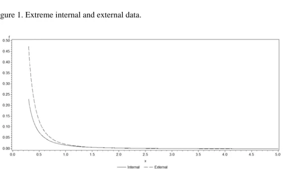
In Figure 1 we show the results of the semiparametric model described in section 2 on the tail of pdf for the internal and the external data set, respectively. This figure shows as distribution of external data is heavier tailed than one of internal data.

Figure 1. Extreme internal and external data.

Source: Bolancé et al. (2012b)

With the aim to estimate Value-at Risk (VaR) and Tail-Value-at-Risk, we estimate four models for the density function of the losses associated with operational risk, named M1, M2, M3 and M4. Model M1 denotes the semiparametric model described in section 2 and will be used for the internal and the external data set, respectively. Models M2 and M3 are mixing models in section 3. In M2 we use transformation parameters estimated with external data to obtain transformed kernel density estimation with internal data. The rescaling procedure is introduced in model M3. This model is similar to M2, but in M3 we use shape transformation parameters estimated with external data and the scale transformation parameter estimated with internal data.

Finally, model M4 is the benchmark model with a Weibull assumption on the severity estimated with internal data.

From the severity density function, we estimate the distribution of total operational risk. We assume that the number of losses over a fixed time period follows a Poisson process. We assume that the annual number of internal losses that have been reported has mean equal 30, then we can assume that the annual number of internal losses follows a Poisson process with maximum likelihood estimated parameter 30. We denote the annual simulated reported frequencies by with 1, … and number of simulations 10,000. After correcting for underreporting, we estimate the expected number of occurred claims as ⁄ , where

and we denote the annual simulated occurred frequencies by . The value of for each estimated model is around 126 occurred losses.

For each annual simulated reported frequencies we draw random uniformly distributed samples 0,1 for 1, … , and obtain loss sizes taken from the inverse estimated cumulative distribution function of the severity distribution of reported claims , this function is obtained integrating the estimated densities function calculate with the different models: M1, M2, M3 and M4. The outcome are the simulated reported annual total losses

denoted by ∑ , 1, … , , where is the inverse of the cumulative

distribution function.

We do the same using the annual simulated occurred frequencies and cumulative distribution function with underreporting correction. The simulated occurred annual total losses

are ∑ , 1, … , , with 0,1 for 1, … , and is the

inverse of the cumulative distribution function obtained integrating the estimated densities from the four proposed models with underreporting correction, as we describe in section 4.

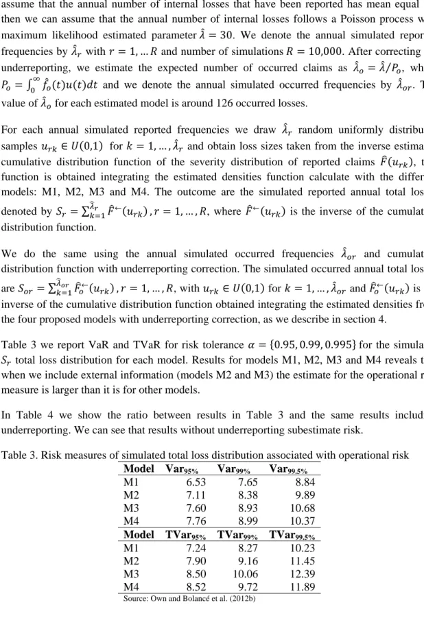
Table 3 we report VaR and TVaR for risk tolerance 0.95, 0.99, 0.995 for the simulated total loss distribution for each model. Results for models M1, M2, M3 and M4 reveals that when we include external information (models M2 and M3) the estimate for the operational risk measure is larger than it is for other models.

In Table 4 we show the ratio between results in Table 3 and the same results including underreporting. We can see that results without underreporting subestimate risk.

Table 3. Risk measures of simulated total loss distribution associated with operational risk

Model Var95% Var99% Var99.5%

M1 6.53 7.65 8.84

M2 7.11 8.38 9.89

M3 7.60 8.93 10.68

M4 7.76 8.99 10.37

Model TVar95% TVar99% TVar99.5%

M1 7.24 8.27 10.23

M2 7.90 9.16 11.45

M3 8.50 10.06 12.39

M4 8.52 9.72 11.89

Table 4. Ratio between risk measures with underreporting and without underreporting.

Model Var95% Var99% Var99.5%

M1 2.41 2.92 4.91

M2 3.24 5.38 9.18

M3 3.38 5.64 8.81

M4 2.03 1.94 1.89

Model TVar95% TVar99% TVar99.5%

M1 2.83 3.84 6.78

M2 4.64 7.02 9.58

M3 4.75 6.96 9.13

M4 1.98 1.91 2.02

6 Discussion

Our recommendation is to pay attention to underreporting whereas model selection for combining internal and external data is especially relevant only when the tolerance level is high, which is when the quantile for assessing risk if high.

Our application handles the problem underreporting together with the mixing of internal and external data. It clearly shows that failure to account for underreporting may lead to a substantial underestimation of operational risk. The use of external data information can easily be incorporated in our modeling approach. So, even if the underlying theoretical foundation is technically difficult, the intuition and the practical implementation of operational risk models is very straightforward.

Our method also addresses the statistical problem of estimating a density function with extreme values and then how to combine data sources, while accounting for operational risk underreporting. Underreporting, which is a feature that practitioners admit is the most dangerous problem of operational risk data quality, has generally been much ignored in the specialized literature. More details on the underlying methodology are to be found in Bolance et al. (2012b), but the applications presented there had not shown the combined effect of mixing internal and external data and the issue of underreporting at the same time.

References

Ashby, S., 2011, “Risk Management and the Global Banking Crisis: Lessons for Insurance Solvency Regulation,” The Geneva Papers on Risk and Insurance: Issues and Practice, 36, 3, 330-347

Bolancé, C., Ayuso, M. and M. Guillén, 2012a, “A nonparametric approach to analyzing operational risk with an application to insurance fraud,” TheJournal of Operational Risk, 7, 1, 57–75

Bolancé, C., Guillén, M. and J.P. Nielsen, 2003, “Kernel density estimation of actuarial loss functions,” Insurance: Mathematics and Economics, 32, 1, 19–36

Bolancé, C., Guillén, M. and J.P. Nielsen, 2008 “Inverse Beta transformation in kernel density estimation,” Statistics & Probability Letters, 78, 1757–1764

Bolancé, C., Guillén, M., Gustafsson, J. and Nielsen, J.P., 2012b, Quantitative Operational Risk Models, Chapman and Hall/CRC finance series, New York

Bolancé, C., Guillén, M., Pelican, E. and Vernic, R., 2008, “Skewed bivariate models and nonparametric estimation for the CTE risk measure,” Insurance: Mathematics and Economics, 43, 3, 386-393

Buch-Kromann, T. and Nielsen, J.P., 2012, “Multivariate density estimation using dimension reducing information and tail flattening transformations for truncated and censored data,” Annals of the Institute of Mathematical Statistics, 48, 1, 167-192

Buch-Kromann, T., Guillén, M., Linton, O. and Nielsen, J.P., 2011, “Multivariate density estimation using dimension reducing information and tail flattening transformations,” Insurance: Mathematics and Economics, 48, 1, 99-110

Buch-Larsen, T., Nielsen, J.P., Guillén, M. and C. Bolancé, 2005, “Kernel density estimation for heavy-tailed distributions using the Champernowne transformation,” Statistics, 39, 6, 503–518

Carrillo, S., Gzyl, H. and Tagliani, A., 2012, “Reconstructing heavy-tailed distributions by splicing with maximum entropy in the mean,” TheJournal of Operational Risk, 7, 2, 3–15

Cavallo, A., Rosenthal, B., Wang, X. and Yan, J., 2012, “Treatment of the data collection threshold in operational risk: a case study using the lognormal distribution,” TheJournal of Operational Risk, 7, 1, 3-38

Cope, E. W., 2012, “Combining scenario analysis with loss data in operational risk quantification,” The Journal of Operational Risk, 7, 1, 39-56

Dahen, H. and G. Dionne, 2007, “Scaling models for the severity and frequency of external operational loss data,” Journal of Banking & Finance, 34, 7, 1484–1496

Dhaene, J., Tsanakas, A., Valdez, E.A. and Vanduffel, S., 2011, “Optimal capital allocation principles,” The Journal of Risk and Insurance, 79, 1, 1-28

Embrechts, P., Kluppelberg, C. and T. Mikosch, 2006, Modelling extremal events for insurance and finance, Springer, Berlin

Eling, M., 2012, “Fitting insurance claims to skewed distributions: Are the skew-normal and skew-student good models?,” Insurance: Mathematics and Economics, 51, 2, 239-248

Feng, J., Li, J. Gao, L. and Hua, Z., 2012, “A combination model for operational risk estimation in a Chinese banking industry case,” The Journal of Operational Risk, 7, 2, 17-39

Gatzert, N. and Wesker, H., 2012, “A Comparative Assessment of Basel II-III and Solvency II,” The Geneva Papers on Risk and Insurance: Issues and Practice, 37, 3, 539-570

Guillén, M., Gustafsson, J. and J.P. Nielsen, 2008, “Combining underreported internal and external data for operational risk measurement,” The Journal of Operational Risk, 3, 4, 3–24

Gustafsson, J. and J.P. Nielsen, 2008 “A mixing model for operational risk,” The Journal of Operational Risk, 3, 3, 25–37

Gustafsson, J., Pritchard, P., Nielsen, J.P., and D. Roberts, 2006, “Quantifying operational risk guided by kernel smoothing and continuous credibility: A practitioners view,” The Journal of Operational Risk, 1, 1, 43–55 Gzyl, H., 2011, “Determining the total loss distribution from the moments of the exponential of the compound loss,”

The Journal of Operational Risk, 6, 3, 3-13

Horbenko, N., Ruckeschel, P. and Bae, T., 2011, “Robust estimation of operational risk,” The Journal of Operational Risk, 6, 2, 3-30

Hoyt, R.E. and Liebenberg, A.P., 2011, “The value of enterprise risk management,” The Journal of Risk and Insurance, 78, 4, 795-822

Peters, G.W., and S.A Sisson, 2006, “Baysian inference, Monte Carlo sampling and operational risk,” The Journal of Operational Risk, 4, 2, 69–104

Peters, G.W., Shevchenko, P.V. and M.V. Wüthrich,, 2009, “Dynamic operational risk: modeling dependence and combining different sources of information.,” The Journal of Operational Risk, 1, 3, 27–50

Pigeon, M. and Denuit, M., 2011, “Composite Lognormal–Pareto model with random threshold,” Scandinavian Actuarial Journal, 3, 177-192