Network Performance: Does It Really Matter To
Users And By How Much?
Ramesh K. Sitaraman
University of Massachusetts, Amherst and Akamai Technologies Inc. Email: [email protected]
Abstract—Network performance has been the subject of much research over the past decades. However, the impact of perfor-mance on a network’s users is much less understood from a scientific standpoint. This gap in our knowledge is particularly stark since the primary role of real-world network performance is to increase user satisfaction, and encourage user behaviors that lead to greater monetization. As an example, consider the video delivery ecosystem consisting of content delivery net-works (CDNs), video content providers, and their users. Content providers use CDNs to deliver videos to their users with higher performance. In turn, content providers expect the higher quality stream delivery to translate into lesser viewer abandonment, greater viewer engagement, and more repeat viewers, all of which lead to greater profits. Thus, whether and to what extent video performance causally impacts viewer behavior is at the core of the online video ecosystem. We review our prior research that for the first time derives the causal impact of video performance as measured by failures, startup delay and freezes on metrics of user behavior that content providers care about. A centerpiece of our work is a novel technique based on quasi-experimental designs (QEDs) that enable us to derive cause-effect relationships between performance and behavior with a greater degree of confidence than just correlation. While QEDs are used extensively in the social and medical sciences, we adapt the technique for network measurement research that is likely to be useful in a number of other contexts. We hypothesize that the availability of large amounts of performance and behavioral data and the develop-ment of novel analytical tools will finally put the users back at the center of network performance research, revolutionizing both how networks are architected for performance and how business models are evolved for real-world networks.
I. INTRODUCTION
Large distributed network services are at core of a wide range of human activity. Billions of users routinely interact with networks of various kinds for commerce, entertainment, news, and social networking. Networks are often designed with a notion of performancein mind. The notion of performance of a network is related to the service that it provides it’s users. For instance, a content delivery network (CDN) provides the service of delivering content to users on behalf of content providers [5], [16]. The notion of performance of a CDN depends on the type of content that it delivers. For a CDN that delivers an e-commerce site to users, performance is typically measured by page availability and page download times. Availability measures the percent of time a user is able to download a page of the web site without failure, and download time measures how quickly the page is downloaded and rendered by the browser. CDNs for e-commerce are
often architected to optimize these metrics. Likewise, a CDN designed to deliver videos has a somewhat different notion of performance. Such as CDN is often measured by whether the video is available without failures (availability), whether the video starts up quickly (startup delay), and whether the video plays without freezing (rebuffers). Customarily, a CDN for me-dia is architected to provide highest performance along these axes. Other examples of network services include cloud ser-vices, Software-as-a-Service (SaaS) platforms, Infratructure-as-a-Service (IaaS) platforms, and online gaming. Each such network service is implemented with a notion of performance that is often measured and optimized.
Real-world network services also have abusiness rationale
for their existence. From a business context, the role of net-work performance is simply to increase user satisfaction and encourage user behaviors that lead to greater monetization. For instance, the goal of an e-commerce provider is to encourage users to shop more and buy more on their website, leading greater revenues and profits. Likewise, a content provider who provides online videos such as news, sports or movies wants to decrease the fraction of viewers who abandon their videos, to increase the amount of time each video is watched, and to improve the likelihood that viewers return to their web site over time. A video content provider relies on advertisement or subscription revenues that depend on greater opportunities for ad insertion and a larger viewership. Thus, all three goals of reducing abandonment, increasing engagement, and improving repeat viewership lead to favorable business outcomes for the content provider,
A. The Virtuous Cycle
At the center of the economic life of a network service, there is often a virtuous cycle where enhancing the performance of the network favorably impacts the manner in which users interact with the service. This leads to greater profits for the enterprise that uses the network service. The increased profits, in turn, justify current and future investments in improving the network performance of the service.
For instance, consider a gaming company that uses a network service to deliver online games to their users. Key network performance metrics for online games include the time for a user to start a new game and the speed at which users playing the game can interact with each other. Improving performance is expected to attract more users who play longer, both of which relate directly to the business objectives of the 978-1-4673-5494-3/13/$31.00 c 2013 IEEE
**justified by improved business metrics "Improved" User Behavior Network Service Provider (CDN)
Content Provider Users
Improved Performance Investment**
$
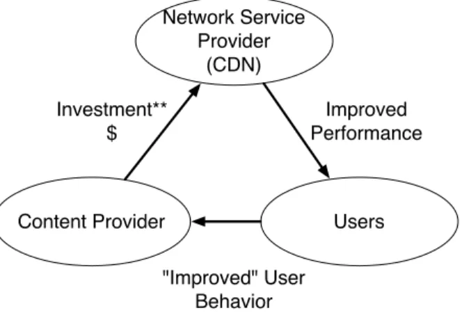
Fig. 1: The Virtuous Cycle of Content Delivery. gaming company.
As another example of a virtuous cycle, consider the content delivery ecosystem. There is a virtuous cycle that links the content provider, network service provider (i.e., CDN) and the users (c.f Figure 1). Content providers typically invest in a CDN to deliver videos to their users with higher performance. The expectation of the content providers is that the higher performance enjoyed by their users will cause changes in the viewing habits of their user population in ways that are favorable to their business, i.e., users will abandon less, watch more, and return more often.
While network performance and its associated metrics have been well-studied in isolation, the critical question is what impact do those metrics have on user behavior. For instance, if web pages download faster would users shop more on an e-commerce site? If users experience less failures, are they more likely to come back to the same web site? If videos start up slowly, would more viewers abandon the videos? Would frequent freezes during video playback lead to viewers watching less of the video? The critical link in the virtuous cycle is the impact of network performance on user behavior. This link is often the most importantwhile at the same time the least understoodfrom a truly scientific standpoint.
B. Understanding the Missing Link
A scientific understanding of the impact of network perfor-mance on user behavior is the primary focus of this paper. The fact that better performance would have a positive impact on users would seem almost tautological. So, why study this at all? The key reason is that any study of the impact must have two characteristics to be useful: it must be quantifiableand it must establishcausalityto an acceptable degree.
1) Quantifiability: Let us examine what we mean by “quan-tifiable”. Taking video delivery as an example, suppose we hypothesize that video freezes due to rebuffering cause users to play fewer minutes of the video. There is certainly value in establishing the hypothesis as is. However, it is more valuable to show quantitatively that an x% increase in video freezes
causes a y% decrease in the minutes of video watched. A quantitative statement of this sort enables the content provider to estimate the potential business impact of reducing freezes and to determine if it is worth obtaining that extra bit of performance. As a concrete example1, suppose that a content provider with an ad-supported business model knows that video freezes cause viewers to watch 5% fewer minutes. Using this information, the content provider can estimate the fewer ad impressions that result from the fewer minutes of video played. That in turn can be translated into the amount of ad revenues lost due to video freezes. This enables the content provider to quantitatively justify investment in a higher performing network service (such as those offered by a CDN) to eliminate the freezes. Thus, a quantitative understanding of the impact of performance on users closes the virtuous cycle, enabling an understanding of the business value of network performance.
2) Causality: The impact of performance on the user must be established in a causal manner. The virtuous cycle is one of cause and effect. A content provider investing in additional performance needs hard evidence that his/her investment in additional performance was thecausefor the favorable change in viewer behavior, and not just something that would have happened for other reasons anyway.
Establishing causality can be tricky as there are both secular trends and confounding factors that can obfuscate a causal con-clusion. As an example of secular trends, consider that some metrics have generally trended higher over the past several years, albeit with varying rates of growth. The e-commerce industry tracks a key user behavioral metric called conversion rate which is the fraction of user visits to an e-commerce site that result in the user buying a product from the site. For many online retailers, conversion rates have been increasing over the past several years due to improved checkout procedures, and better product selection [20]. Suppose now that the online retailer makes improvements to the performance of their e-commerce web site. Further, suppose that conversion rates increase after the performance enhancements are complete. Is the increase due to enhanced performance? Or, is it just the secular trend of higher conversion rates over time?
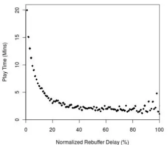
As another example, in a recent study [11] we examined almost 23 million video playbacks over 10 days and correlated the amount of freezes experienced by the viewer due to rebuffering and the number of minutes of the video that the viewer watched (c.f Figure 2). While it is clear from the figure that play time and rebuffer delay are inversely correlated, can we conclude on this basis that video rebuffering caused the viewers to watch fewer minutes of the video?
Most network measurement work stop at correlations, but it is generally not sufficient evidence for causality. As the popular dictum states “correlation is not causation”. Note that it is generally not possible to prove causality beyond any
doubt, in this or any other scientific endeavor. However, it behooves us to eliminate the common threats to causality, so 1The example is highly simplified for illustration. The actual business impact computation is likely based on a more complex revenue model.
Fig. 2: Correlation of normalized rebuffer delay with play time. Normalized rebuffer delay is the total time the video froze due to rebuffering divided by the duration of the video [11]. that we can have a greater confidence in a causal conclusion. For instance, a threat to a causal conclusion based on the observed correlation in Figure 2 is the following plausible
scenario. Suppose that viewers who live in wealthier geo-graphic locations have better broadband connectivity. Due to their superior network connectivity their videos tend to freeze less often due to rebuffering. Further, suppose that those same viewers can afford access to more captivating premium video content that makes them watch longer. This scenario can result in the amount of rebuffering and the play time to be inversely correlated without the first causing the second. In fact in this scenario, more rebuffering and less play time are both caused by a set of confounding factors. Geography, network connectivity and the content itself are almost always confounding factors as each capture aspects of the video viewing experience that must be accounted for in any causal study of video performance and viewer behavior.
C. Our Research Enablers: Big Data and New Techniques
Our research is focused on the urgent need to evolve a scientific foundation for understanding the impact of network performance on users in a quantitative and causal manner, thereby establishing the missing link and closing the virtuous cycle. Such research would not have been possible even a few years ago for lack of large-scale measurements of performance and user behavior. But, today the time is ripe since for the first time large amounts of user behavior and user-perceived performance data can be measured, collected, and analyzed.
In the case of online videos, when we built the first CDNs in the late 1990’s and the early 2000’s, accurate performance information could only be obtained through measurement
agents deployed around the globe. The agents incorporated a media player that repeatedly played and measured streams to report on streaming performance [21], [2]. Accurate per-formance or behavioral measurements from actual users in the wild were unachievable in any large scale. The advent of customizable players for most major streaming formats such as Flash, Silverlight, iOS/Quicktime and HTML5 changed all that. It is now possible to integrate an analytics plugin that runs inside the user’s media player [1] that measures and reports both user actions (play, pause, rewind, browser close, etc) and performance metrics (startup delay, rebufffering events, bandwidth, etc). In our work in [11], we relied on large-scale anonymized data collected from actual users playing videos from around the world using media players that incorporate the widely-used Akamai media analytics plug-in.
It is also worth noting that the availability of client-side data from media players has enabled recent key studies such as [6] that shows several correlational relationships between quality, content type, and play time. A recent sequel to the above work [15] also uses client-side data to suggest enhancements to video delivery. Besides media players, several other networked clients such as browsers and download managers running on a multitude of devices are also producing enormous amounts of behavioral and performance information like never before. This opens up exciting possibilities for studying a variety of networks from the standpoint of relating performance to user behavior and closing the virtuous cycle.
II. EXPERIMENTALTECHNIQUES
The availability of “big data” is a necessary but not a suf-ficient condition for achieving our research goals. We need to discover new experimental techniques that can quantitatively extract cause-effect relationships that can be hidden in large amounts of network data. We focus on those techniques next. Discovering quantitative and causal relationships is at the heart of every scientific endeavor. In striving to establish such relationships in network measurement, it behooves us to examine the techniques utilized in the physical, medical and social sciences. A precise mathematical definition of cause, effect, and a causal relationship has eluded philosophers for centuries. The 19th century philosopher John Stuart Mill
describes a causal relationship using three criteria [19] that resonates with our own modern conception of causation:
1) The cause must precede the effect. 2) The cause must be related to the effect.
3) We can find no plausible alternative to the effect other than the cause.
In most cases, the first criterion is easily verified. For instance, in our domain it is easy to verify that the performance degrada-tion (say, video freezes) occurs before an user acdegrada-tion (say, user stops playing the video). The second criterion can typically be established by showing that the cause and effect tend to occur together, i.e., that they are correlated (for instance, Figure 2). But, one cannot conclude causality without establishing the third criterion. A plausible alternate explanation in our domain, and verily many other scientific domains, takes the form of
confounding factors. Suppose we want to establish a causal relationship between two variables A and B. A confounding
factor is a third variable C that could cause both A and B
giving rise to a correlation between them, but that correlation does not necessarily imply a causation.
Confounding factors can often be subtle. In a well-known case in recent medical literature, researchers claimed that children who sleep with their lights on have a greater tendency to develop myopia in later life [17]. It was later discovered that the researchers had not identified a critical confounding factor: the presence or absence of myopia in the parents of the studied children. As it turns out, myopic parents had a greater tendency to leave the light on in their children’s bedroom, since it was harder for them to see without those lights. In addition, myopic parents have a genetic disposition to myopia that make their children more likely to be myopic later in life. Subsequently, accounting for the additional confounding factor, altered the prior conclusion of the causal effect of bedroom lights on myopia.
The critical task of designing experiments in our domain is a careful elimination of alternate explanations to satisfy Mill’s third criterion for causality. An intuitively satisfying way for satisfying the third criteria is by establishing acounterfactual. That is, besides showing that if the cause happens the effect happens, you also establish the counterfactual that if the cause
does not happen the effectdoes nothappen. Unfortunately, a exact counterfactual can seldom be established. For instance, in our prior example, a child either sleeps with the lights on or does not, i.e., it can’t simultaneously do both. One can view the different experimental techniques that we will discuss next as trying to approximate the counterfactual, since an exact counterfactual is impossible.
A. Randomized Experiments
The classical technique for establishing causal, quantitative results in the medical and social sciences is the randomized experiment popularized by the great statistician Sir Ronald Fisher in the 1920’s [9]. To establish that A causes B, the
experimental units2 are randomly divided into groups. One group is “treated3” with A and the other control group is left “untreated”. By observing the relative presence of the effectBin the two groups yields positive or negative evidence for the causal link between A and B. The key element of a randomized experiment is the randomized assignment of the treatment to the experimental units. The randomized assignment is independent of any other factors and so the presence of confounding factors are statistically identical in both the treated and control groups. Thus, the effect of the confounding factors are nullified in a statistical sense.
While randomized experiments have their appeal, they are hard to implement in our network performance measurement 2An experimental unit is one member of the set of entities being ex-perimented with. In our case, an experimental unit could be a user, or a combination of a user watching a video.
3It is customary to use medical parlance by referring to the cause as “treatment”, since in the medical sciences experimentation often involves discovering if a treatment can causally effect a cured outcome.
context. In our study of the impact of network performance on users, the “treatment” is performance characteristics such as startup delay or freezes experienced by a user. A random-ized experiment must therefore induce poor performance for viewers in the treated group and provide good performance for users in the control group. It is technically and operationally hard to introduce performance degradation in a controlled manner for a large groups of actual users in the wild on the Internet. Further, even if possible, it would require changes to the existing software of a network service for the purpose of an experiment and is likely expensive. Finally, it may not even be ethical or legal to introduce performance degradation for users without their consent. All of this makes it well-near impossible to conduct a truly randomized experiment involving a large audience of users for the purposes of understanding the impact of performance on behavior.
It is worth noting however that there are other contexts in network services where randomized experiments, or approx-imations thereof, are used successfully. A common form is A/B testing or multivariate testing [10] that is used for online marketing campaigns where two randomly chosen groups are given two different marketing offers and the response rate of these groups is measured to determine the better marketing strategy. A/B testing is also routinely used by large e-commerce providers like Amazon to design their websites, to determine shopping cart features, to decide on product placement on the page, and even to determine what wordings to use on the buttons, all with the goal of increasing the conversion rate funnel [8].
B. Quasi-Experiments
Given the difficulty of doing large-scale randomized exper-iments in our network performance context, we turn to the notion of a quasi-experiment. The key manner in which a quasi-experiment is different from a randomized one is that the former does not require the experimenter to implement randomized assignment. In domains such as ours where it is not possible to control who gets treatment (i.e., poor performance), we find quasi-experiments especially suitable. Intuitively, a quasi-experiment tries to satisfy Mill’s third criterion for causality by doing the following two steps.
1) Explicitly considering possible threats to a causal con-clusion. This typically includes enumerating possible confounding factors that could explain a correlation between the cause and the effect.
2) Designing the experiment so as to eliminate those threats. Once the confounding factors are identified, they are neutralized by explicitly designing a suitable experiment. For instance, the experiment can construct a treatment group and control group that are impacted similarly by the confounding factors, thereby eliminating their influence on the outcome.
By considering and eliminating threats to causality, you pro-vide greater epro-vidence for a causal conclusion. There is always the possibility that there exist undiscovered or unmeasurable confounding factors that remain as potential threats. This is
possibility inherent in much of scientific inference and remains a possibility in our studies.
A key contribution of our work in [11] is adapting the notion of a quasi-experiment for studying network performance. However, even though quasi-experiments have a been seldom used to study computer systems prior to our work, it has a long and distinguished history in the social and medical sciences. A situation analogous to ours where randomized experiments are hard or impossible and quasi-experiments are desirable occurs frequently in the social and medical sciences. For instance, there is often little control on who receives the treatment and who does not. For this reason, quasi-experiments are among the most widely used techniques for experimentation in these disciplines.
Take for example the question of whether a child exposed to bedroom lights is more likely to become myopic in later life. If a randomized experiment were possible, we would randomly decide which children have their lights turned on at night and which children do not. A sufficient large experimental sample will then average out any confounding factors such as the parent’s myopia. However, such control is impossible to achieve. Indeed, the experimenter has no control over which children get exposed to bedroom lights and which do not, ruling out the possibility of a randomized experiment. In such a case, a quasi-experiment where treated and control groups are judiciously chosen from among the observed population so as to account for confounding factors is the primary option.
The early history of quasi-experiments date back to the
18th century Scottish physician James Lind who performed
one of the first clinical experiments in the history of modern medicine to study the effects of citrus fruit on scurvy [7]. More recently, the notion of a quasi-experiment was formalized and popularized by Campbell and Stanley in their classic book [3]. While a number of different quasi-experimental designs (abbreviated as QED) exist, we now examine a design technique that is particularly suited for our problem domain of analyzing video quality’s impact on users.
C. The Matching Technique for Quasi-Experimental Design
Suppose that we wanted to show that cause A produces
an effect B. Suppose further that we are aware of significant
confounding factors C that could cause both A and B.
We design a matched quasi-experiment by choosing a large number of pairs of experimental units ht, ui where unit t
has cause A and is part of the treated group. The other unit
u is untreated without A and is part of the control group. Further, the matched units t and u have are as identical as possible on the confounding factors C. With each pair, we associate an outcome(t, u) which is positive (say) if the pair provides positive evidence for the hypothesis that A causes
B, negative if the pair provides negative evidence for the
hypothesis, and zero otherwise. Aggregating the outcomes for a large of number of matched pairs M, we compute
Net Outcome =
P
ht,ui2Moutcome(t, u)
|M| .
With a proper choice of the outcome function, the net outcome of the experiment provides an assessment of whether or not a purported causeA produces an effectB. Further, the
magni-tude of the net outcome can provide a quantitative assessment of that impact. Since the matched pairs have similar values for the confounding factors, the effect of these factors on the final outcome is diminished. In other words, the untreated control group is “similar” to the treated group on the confounding factors and hence provides counterfactual evidence of what might happen if the causeA had not occurred, all else being the same. Such counterfactual evidence is essential for a causal inference.
The matching technique has intuitive appeal and hence has been used widely. The classic studies of twins in the medical and social sciences are powerful examples of QEDs that use matching. For instance, a ground-breaking study of the impact of schooling on future wages [12] paired up 298 genetically-identical twins who differed in their level of schooling. The study concluded that each additional year of schooling increases the wages by 12-16%. The use of twins helps eliminate a host of confounding factors that have basis in either genetics or family background, helping isolate the differing schooling (cause) as a prime determinant of the wages (effect). However, in most QEDs that use matching, the experimental units cannot be matched as exactly as in the case of identical twins. But, rather the matched pairs are similar rather than identical.
III. QEDS FORVIDEOPERFORMANCEIMPACTANALYSIS We show how quasi-experiments that use matching can be designed for determining the impact of video streaming performance on viewers. The key idea is creating pairs of viewers who are identical with respect to confounding factors such as geography, connection type and the watched content, but differ in whether or not they received poor performance (i.e., the treatment). The designs and results in this section are from our work in [11].
A. The Data
The data sets that we use for our analysis are collected from a large cross section of actual users around the world who play videos using media players that incorporate the widely-deployed Akamai’s client-side media analytics plug in4. When content providers build their media player, they can choose to incorporate the plugin that provides an accurate means for measuring a variety of stream performance and viewer behav-ioral metrics. When the viewer uses the media player to play a video, the plugin is loaded at the client-side and it “listens” and records a variety of events that can then be used to stitch together an accurate picture of the playback. For instance, player transitions between the startup, rebuffering, seek, pause, and play states are recorded so that one may compute the relevant metrics. Properties of the playback, such as the current 4While all our data is from media players that are instrumented with Akamai’s client-side media analytics plugin, the actual delivery of the streams could have usedanyplatform and not necessarily just Akamai’s CDN.
bitrate, bitrate switching, and state of the player’s data buffer are also recorded. Further, viewer-initiated actions that lead to abandonment such as closing the browser or browser tab, clicking on a different link, etc can also be accurately captured. Once the metrics are captured by the plugin, the information is “beaconed” to an analytics backend that can process huge volumes of data. From every media player at the beginning and end of every view, the relevant measurements are sent to the analytics backend. Further, incremental updates are sent at a configurable periodicity even as the video is playing. Our data set is extensive and captures 23 million video plays by 6.7 million unique viewers who watched for a total of 216 million minutes over 10 days. The videos belong to a representative slice of 12 content providers belonging to a variety of verticals including news, entertainment, and movies.The users too came from a wide cross-section of geographies including North America, Europe, and Asia. More details on the properties of this data set is found in [11].
B. The Quasi-Experiment for Viewer Engagement
We revisit our earlier question on whether video freezes due to rebuffering can decrease a viewer’s engagement with the content. A good measure of viewer engagement is the amount time a viewer plays a video. So, we would like to establish that the following assertion holds in a causal and quantitative fashion.
Assertion 1([11]). An increase in (normalized) rebuffer delay can cause a decrease in play time.
The observed negative correlation between play time and normalized rebuffer delay in Figure 2 is indicative but not sufficient to imply causality as there are threats such as the one outlined earlier that involve potentialconfounding factors such as the content itself, the geography of the user, and the connection type of the user. We examine each of the potential confounds in turn.
• Content. Play time is clearly impacted by interest level of the viewer in the video content. Interest level could also vary at different parts of the video. Some parts could be interesting, such as when a plot is revealed, and other parts could be boring, such as when the story line drags on. A viewer who had good a quality stream may quit during a boring part, or might hold on during an interesting part despite poor quality. Thus, the effect of the content itself needs to be neutralized by comparing viewers who are watching the same content and in fact the same portionof that content.
• Geography. Where the user lives is also a potential confounding factor. Geography does of course influence the interest level of the user in the video. For instance, Brazilian viewers might be more interested in soccer world cup videos than Indian viewers, even more so if the video is of a game where Brazil is playing. Studies have shown that different countries have different tolerance levels in social situations in the physical world, such as the levels of patience for waiting in queues for services.
Treated (video froze for ≥ 1%
of duration)
Control or Untreated (No Freezes) Same geography,
connection type, same point in time
within same video Outcome For each pair, outcome =
(playtime(untreated) – playtime(treated))/ video duration
Fig. 3: Matched Quasi-Experimental Design for Viewer En-gagement with treatment level = 1%. The paired viewers
are from the same geography, have the same connection type, and are watching the same portion of the same video, but differ on the rebuffering that they experienced.
For the same reasons, it is conceivable that geography also influences a viewer’s tolerance to video performance degradation in the virtual world.
• Connection Type.The connection type of the user pro-vides information on whether the user is on a mobile wireless connection or a wired connection, the latter can be further subdivided into dialup, DSL, cable, or fiber (such as Verizon’s XFINITY or AT&T’s FIOS). The con-nection type primarily captures network characteristics such as available bandwidth, e.g., fiber connections have significantly more bandwidth than mobile.
Matching Algorithm. We now present the matching algorithm from [11] for creating a large number of pairs of viewers who are similar on all three (potential) confounding factors, but dif-fer in the performance that they experienced (c.f Figure 3).The treatment set T consists of all video views that suffered
normalized rebuffer delay more than a certain threshold %.
Given a value of as input, the treated views are matched with untreated views that did not experience rebuffering as follows.
1) Match step.We form a set of matched pairsMas follows. LetT be the set of all video views with a normalized rebuffer delay of at least %. For each view u in T, suppose that
u reaches the normalized rebuffer delay threshold % when viewing the tth second of the video, i.e., view u receives
treatment after watching the firsttseconds of the video, though more of the video could have been played after that point. We pick a view v uniformly and randomly from the set of all
possible views such that
a) the viewer ofv has the same geography, connection type, and is watching the same video as the viewer of u.
b) Viewvhas played tilltseconds of the video without rebuffering. This step ensures that bothuandvhave both watched to the same point in the video, the only difference being that u received treatment at
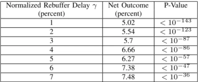
Normalized Rebuffer Delay Net Outcome P-Value (percent) (percent) 1 5.02 <10 143 2 5.54 <10 123 3 5.7 <10 87 4 6.66 <10 86 5 6.27 <10 57 6 7.38 <10 47 7 7.48 <10 36
TABLE I: On average, a viewer who experienced more re-buffering watched less minutes of the video than an identical viewer watching the same video with no rebuffering. Further, the p-values indicate that the results are statistically significant. good performance at the same point. That is, both
uandv have viewed the same content and the only
difference between them is one had rebuffering and the other did not.
2) Score step. For each pair(u, v)2M, we compute
outcome(u, v) =play time of v play time of u
video duration . N et Outcome= P (u,v)2Moutcome(u, v) |M| ! ⇥100.
The net outcome of the matching algorithm can be viewed as the difference in the play time of u and v expressed
as a percent of the video duration. That is, net outcome measures the additional amount of the video the viewer with good performance watched over a similar viewer with bad performance. Table I shows that an average viewer who experienced normalized rebuffer delay of at least 1% played 5.02% fewer minutes of the video, compared to a viewer who experienced no rebuffering at all. There is a general upward trend in the net outcome when the treatment gets harsher with increasing values of .Note that QEDs that use matching give exactly the kind of quantitative and causal answers that we argued in Section I-B are of great value to a content provider. C. Some Finer Points in our Matched QED Analysis
We discuss some finer points in our approach described above to using QEDs to determine the impact of performance on users.
1) Are the results statistically significant?: As with any statistical result, it is important to understand whether it is statistically significant. Assessment of statistical significance often involves asking how possible it is that the treatment had no effect but the net outcome happened just by random chance. In the standard terminology of hypothesis testing [14], we state a null hypothesis Ho that the cause (i.e., treatment)
has no impact on the outcome. We then compute the “p-value” defined to be the probability of the observed net outcomegiven
that the null hypothesisHoholds. Thus, intuitively, the p-value
represents the odds of the net outcome happening by chance. A “low” p-value lets us reject the null hypothesis, bolstering our conclusions from the QED analysis as being statistically significant. However, a “high” p-value would not allow us to
reject the null hypothesis. That is, the QED results could have happened through random chance with a “sufficiently” high probability that we cannot rejectHo. In this case, we conclude
that the results from the QED analysis are not statistically significant.
The definition of what constitutes a “low” p-value for a result to be considered statistically significant is somewhat arbitrary. It is customary in the medical sciences to conclude that a treatment is effective if the p-value is at most0.05. The
choice of0.05as the significance level is largely cultural and
can be traced back to the classical book of R.A. Fisher in 1925 that also popularized randomized experiments [9]. Some have recently argued that the significance level must be much smaller. We concur and we suggest a more stringent 0.001
as our significance level, a level achievable in our field given the large amount of experimental subjects (tens of thousands treated-untreated pairs) but is rarely achievable in medicine with human subjects (usually in the order of hundreds of treated-untreated pairs).
The primary technique that we employ in our QEDs for evaluating the p-value, and hence statistical significance, is the sign test that is a non-parametric test that makes no distributional assumptions [22] and is well-suited for evalu-ating matched pairs in our QED setting. For each randomly matched pair(u, v), whereureceived treatment andvdid not
receive treatment, we observe thatoutcome(u, v) is positive
if the pair provides positive evidence for the Assertion 1 and the untreated v plays longer than the treated u. Likewise, outcome(u, v) is negative if the pair provides negative evi-dence for the assertion. If the null hypothesisHo holds, then
the treatment or lack thereof has no effect on the outcome and the non-zero values ofoutcome(u, v)are equally likely to be a positive or negative.
We now compute that equals the difference between the number of pairs (u, v) with positive outcome(u, v) and the
number of pairs with a negative outcome(u.v). Letn be the
number of pairs with non-zero outcome values. The probability distribution of can be approximated byBin(n,1/2) n/2
where Bin(n,1/2) is the binomial distribution with n trials
and success probability of1/2for each trial. For an observed
value , the probability that the observed value occurs given that the null hypothesis Ho holds is
P rob( = )P rob(|X n/2| | |),
where the random variable X has a probability distribution Bin(n,1/2). Evaluating the above tail probability bound for
the binomial distribution provides us the required bound on the p-value.
As a concrete example, our quasi-experiment with =
1% shown in Table I yielded 52,028 pairs with non-zero outcomes of which 28,810 had positive values and 23, 218 had negative values. The probability that the observed skew between positive and negative outcomes = 28,810 23,218 = 5592 occurs, given that the null hypothesis Ho
holds, is obtained by bounding the tails of the distribution
number positive (or negative) outcomes. The p-value bounded in this fashion amounts to a very small number of about
1.5⇥10 144, which is much less that the required 0.001.
Hence, we conclude that our results are statistically significant. While the sign test is commonly used with matching QEDs, a different but distribution-specific significance test called the paired T-test may be applicable in other QED situations. A paired T-test uses the Student’s T distribution but requires that
outcome(u, v)has a normal distribution. Since our differential outcome does not have a normal distribution, we rely on the distribution-free non-parametric sign test that is more generally applicable.
2) How close should the matching be?: The closer we can match the chosen variables for the paired experimental units, the more accurate our QED results. In our QED example in Section III-B, we have used exact matches on the portion of the content watched (within 1 second), geography (by country), and connection type (mobile, dsl, cable, or fiber). Since we have very large data sets, we were able to obtain several tens of thousands of matching pairs, yielding statistically significant results. However, when data sets are smaller or when the number of matching variables are large, it is unlikely to find sufficient pairs with exact matches in the data set. In this case, one can perform caliper matching where it is sufficient that the matched factors have values within a specified distance [4]. Different metrics of distance have been used in the social sciences including Mahalanobis distance or nearest neighborhood distance. A common alternative to using distance is to create a composite value from the values of the multiple variables that are to be matched. The composite value is called the propensity score and experimental units with similar scores are matched [18].
3) What about hidden threats and confounds?: With QEDs, and in fact with many other techniques for causal inference, there is always the possibility of factors that could impact the analysis that were not considered. It could be that there are factors that are potentially measurable but were not part of the experimental design, as in the case of the parent’s myopia in our earlier example. Or, perhaps there are factors that are sim-ply hard or impossible to measure. In our video study example, it was hard to measure the geography of a user at a granularity finer than country in many parts of the world. Though one could get argue that a finer measurement (say at the zip code or equivalent level) could provide a better picture of the socio-economic status of the person. And, personal characteristics such as age and sex of a person could not be measured, though any influence of these variables on what videos were watched is already accounted for in our experimental designs. An excluded factor influences the outcome of a QED only if that factor is differentially distributed in the treated and control sets and if that differential distribution actually causes a significant change in the outcome.
As with any other scientific technique, there is no substitute for good experimental design that carefully considers the significant threats and confounds. It is best to view our work on matched QEDs as a framework for eliminating plausible
Fig. 4: Viewers abandon at a higher rate for short videos than for long videos [11].
threatswhen identifiedand to provide greater confidence that a causal conclusion holds. In fact, in general terms, causality can seldom be proved in black-and-white, but only with increasing confidence in shades of grey.
D. Quasi-Experiments for Abandonment and Repeat Viewers
For completeness, we summarize results from other quasi-experiments devised in [11]. In the physical world, it is known that people are more patient if there is a perception of a higher value service at the end of the wait [13]. And, often times the perceived value of a service is also a function of the duration of the service. A 30-minute wait for a 5-minute cab ride frustrates people more than a 30-minute wait for a long plane ride. We wanted to test if the same behavior applies for users waiting for a video to start, i.e., would people be willing to wait longer without abandoning for a long video (say, a movie) than for a short video (say, a news clip). We showed that this was indeed the case (c.f Figure 4). But, we also went one step further and designed a quasi-experiment where each pair of viewers have the same geography and connection type, but differ on the whether they watch a short video (example, news) or a long video (example, movie). With this QED, we showed the following assertion.
Assertion 2 ([11]). Viewers are less tolerant of startup delay for short videos in comparison to longer videos. A viewer watching a short video is 11.5% more likely to abandon sooner during startup than its matching pair watching a long video.
In the physical world, the patience level of users is depen-dent on their expectations. While the transcontinental express train opened in 1876 that traveled from New York City to San Francisco in 83 hours, it was widely heralded as the “lightning
Fig. 5: Viewers who are better connected abandon sooner. express”. No doubt that the transcontinental railroad was a major advance, as it shortened travel time from over a month to only a few days. However, none of us today would have the patience to travel for 83 hours and would find that a frustrating experience What has changed is our expectations of what is an appropriate delay for travel. We wanted to study if the same cultural effect holds in the world of online videos and if people would wait less if theyexpectedtheir videos to startup more quickly. Therefore, we studied the abandonment rate for users on different types of connections ranging from mobile, DSL, cable and fiber. Our basic analysis (c.f. Figure 5) showed that better connected users did in fact have less patience and abandoned more. We then designed a QED where pairs of users are identical with respect to their geography and the watched content but differ on the type of connection used to access the Internet. The outcome of our QED showed a clear distinction between mobile users and the rest. Though some finer distinctions such as between users on DSL and cable had a larger p-value and hence deemed statistically inconclusive. Based on the QED results, we showed the following. Assertion 3 ([11]). Viewers watching videos on a better connected computer or device have less patience for startup delay and so abandon sooner. For instance, a viewer with fiber broadband connectivity is 38.25% more likely to abandon sooner during startup than a similar viewer with mobile connectivity.
Finally, we looked at the effect of a failed visit on repeat viewership. A failed visit is one where a user tries to watch a video but the video fails to play, and the user leaves the content provider’s web site, presumably with some level of frustration. Using QED techniques, we evaluated the impact of a failed visit on the probability that the user comes back to the same
website within a week to play more videos. We randomly created pairs of users where the “treated” user experienced a failed visit and the untreated user did not. The users in each pair need to be made as similar as possible in other regards They were matched on geography, connection type, and content provider that they are visiting. In addition, one needs to be careful not to match an “occasional” visitor to the site, say one who watches on weekends, to a “frequent” visitor, say who watches every day. To capture this additional characteristic we compute that total visits and viewing time
priorto treatment and ensured that these characteristics were similar between the matched pairs. Using this QED, we showed the following assertion.
Assertion 4([11]). A viewer who experienced a failed visit is 2.3% less likely to return to the content provider’s site to view more videos within a week than a similar viewer who did not experience a failed visit.
Our goal in this section was to provide examples of how network performance can be quantitatively and causally linked to user behavior for online videos. The reader is referred to [11] for a more in-depth treatment of these results.
IV. CONCLUSIONS
Understanding the impact of performance on the user is one of the most important but also one of the least understood problems in network performance research. The link between performance and users is key to sustaining the “virtuous cycle” that sustains the economics of a network service. A scientific understanding of the impact needs to be both quantitative and causal. It is now possible to collect, store, and analyze large amounts of performance and user behavior data from network services to the extent not possible even a few years ago. However, sophisticated techniques for experimentation and analysis need to be developed to extract meaningful cause-effect relationships from the measured data.
The causal impact of performance on users is key from two different perspectives. First, network services often need to be engineered to optimize some aspects of performance at the potential cost of others. Understanding the causal impact of the different performance metrics on users is the only quantitative way of making such tradeoffs. Second, the causal impact of performance on users is at the very heart of monetizing a network service. For example, in the case of online videos, the quantitative assessment of the impact provided in [11] helps determine the business value of video performance and shows how modifying aspects of performance can impact the content provider’s business. Further, the study of viewer patience in [11] provides a basis for understanding ad-supported models for online videos that fundamentally rely on viewers waiting patiently through advertisements.
Our initial step towards understanding the impact of perfor-mance on users in [11] represents the first large-scale study of its kind. This work also represents the first use of sophisticated quasi-experimental techniques from the social and medical sciences in the study of network performance. However, it is
clear that what we know today is only the tip of the iceberg. Much remains to be studied in the context of a variety of other network services that are in use today. We hypothesize that the availability of large amounts of performance and behavioral data and the development of better analytical tools will finally put the users back at the center of network performance research, revolutionizing both how networks are architected for performance and how business models are evolved for real-world networks.
ACKNOWLEDGMENT
The author thanks S. Shunmuga Krishnan for insightful discussions about the paper. Any opinions expressed in this work are solely those of the author and not necessarily those of Akamai Technologies.
REFERENCES
[1] Akamai Media Analytics. http://www.akamai.com/html/solutions/ mediaanalytics.html.
[2] Akamai.Stream Analyzer Service Description. http://www.akamai.com/ dl/feature sheets/Stream Analyzer Service Description.pdf.
[3] D.T. Campbell and J.C. Stanley. Experimental and quasi-experimental designs for generalized causal inference. Houghton Mifflin, 1963. [4] W.G. Cochran. The effectiveness of adjustment by subclassification
in removing bias in observational studies. Biometrics, pages 295–313, 1968.
[5] John Dilley, Bruce M. Maggs, Jay Parikh, Harald Prokop, Ramesh K. Sitaraman, and William E. Weihl. Globally distributed content delivery. IEEE Internet Computing, 6(5):50–58, 2002.
[6] Florin Dobrian, Vyas Sekar, Asad Awan, Ion Stoica, Dilip Joseph, Aditya Ganjam, Jibin Zhan, and Hui Zhang. Understanding the impact of video quality on user engagement. In Proceedings of the ACM SIGCOMM Conference on Applications, Technologies, Architectures, and Protocols for Computer Communication, pages 362–373, New York, NY, USA, 2011. ACM.
[7] P.M. Dunn. James Lind (1716-94) of Edinburgh and the treatment of scurvy. Archives of Disease in Childhood-Fetal and Neonatal Edition, 76(1):F64–F65, 1997.
[8] Bryan Eisenberg. Hidden Secrets of the Amazon Shopping Cart. http: //www.grokdotcom.com/2008/02/26/amazon-shopping-cart/.
[9] R.A. Fisher.Statistical methods for research workers. Genesis Publish-ing Pvt Ltd, 1925.
[10] Ron Kohavi, Roger Longbotham, Dan Sommerfield, and Randal M. Henne. Controlled experiments on the web: survey and practical guide. Data Mining and Knowledge Discovery, 18:140–181, 2009.
[11] S. Shunmuga Krishnan and Ramesh K. Sitaraman. Video stream quality impacts viewer behavior: inferring causality using quasi-experimental designs. InProceedings of the ACM Internet Measurement Conference (IMC), pages 211–224, New York, NY, USA, 2012. ACM.
[12] A. Krueger and O. Ashenfelter. Estimates of the economic return to schooling from a new sample of twins. Technical report, National Bureau of Economic Research, 1992.
[13] R.C. Larson. Perspectives on queues: Social justice and the psychology of queueing. Operations Research, pages 895–905, 1987.
[14] E.L. Lehmann and J.P. Romano.Testing statistical hypotheses. Springer Verlag, 2005.
[15] X. Liu, F. Dobrian, H. Milner, J. Jiang, V. Sekar, I. Stoica, and H. Zhang. A case for a coordinated internet video control plane. InProceedings of the ACM SIGCOMM Conference on Applications, Technologies, Architectures, and Protocols for Computer Communication, pages 359– 370, 2012.
[16] E. Nygren, R.K. Sitaraman, and J. Sun. The Akamai Network: A platform for high-performance Internet applications. ACM SIGOPS Operating Systems Review, 44(3):2–19, 2010.
[17] G.E. Quinn, C.H. Shin, M.G. Maguire, R.A. Stone, et al. Myopia and ambient lighting at night. Nature, 399(6732):113–113, 1999.
[18] P.R. Rosenbaum and D.B. Rubin. Constructing a control group using multivariate matched sampling methods that incorporate the propensity score. American Statistician, pages 33–38, 1985.
[19] W.R. Shadish, T.D. Cook, and D.T. Campbell. Experimental and quasi-experimental designs for generalized causal inference.Houghton, Mifflin and Company, 2002.
[20] Shop.org.State of Retailing Online 2011. http://www.shop.org/soro. [21] R.K. Sitaraman and R.W. Barton. Method and apparatus for measuring
stream availability, quality and performance, February 2003. US Patent 7,010,598.
[22] D.A. Wolfe and M. Hollander. Nonparametric statistical methods. Nonparametric statistical methods, 1973.

![Fig. 4: Viewers abandon at a higher rate for short videos than for long videos [11].](https://thumb-us.123doks.com/thumbv2/123dok_us/721943.2590442/8.918.479.813.118.417/fig-viewers-abandon-higher-rate-short-videos-videos.webp)
