Bayesian Inference for Mixtures of Stable Distributions.

Bayesian Inference for

Mixtures of Stable Distributions

Roberto Casarin† ‡ CEREMADE

University Paris IX (Dauphine) and

Dept. of Economics University Ca’ Foscari, Venice

Abstract

In many different fields such as hydrology, telecommunications, physics of condensed matter and finance, the gaussian model results unsatisfactory and reveals difficulties in fitting data with skewness, heavy tails and multimodality. The use of stable distributions allows for modelling skewness and heavy tails but gives rise to inferential problems related to the estimation of the stable distributions’ parameters. Some recent works have proposed characteristic function based estimation method and MCMC simulation based estimation techniques like the MCMC-EM method and the Gibbs sampling method in a full Bayesian approach. The aim of this work is to generalise the stable distribution framework by introducing a model that accounts also for multimodality. In particular we introduce a stable mixture model and a suitable reparametrisation of the mixture, which allow us to make inference on the mixture parameters. We use a full Bayesian approach and MCMC simulation techniques for the estimation of the posterior distribution. Finally we propose some applications of stable mixtures to financial data.

Keywords_{: Mixture model, Stable distributions, Bayesian inference, Gibbs sampling.}

1

Introduction

In many different fields such as hydrology, telecommunications, physics and finance, Gaussian models reveal difficulties in fitting data that exhibits a high degree of heterogeneity; thus stable distributions have been introduced as a generalisation of the Gaussian model. Stable distributions

†_{I’m thankfull to professors C.P. Robert and M. Billio for the suggestions to my Phd. thesis. This work has}

been presented at the Young Statistician Meeting, Cambridge 14-15 April 2003.

‡_{Adress: CEREMADE, University Paris IX (Dauphine), 16 place du Mar´echal de Lattre de Tassigny, 75775}

allow also for infinite variance, skewness and heavy tails. The tails of a stable distribution decay like a power function, allowing extreme events to have higher probability mass than in Gaussian model. For a summary of the properties of the stable distributions see Zoloratev [42] and Samorodnitsky and Taqqu [36], which provide a good theoretical background on heavy-tailed distributions. The practical use of heavy-heavy-tailed distributions in many different fields is well documented in the book of Adler, Feldman and Taqqu [1], which also reviews the estimation techniques.

In finance, the first studies on the hypothesis of stable distributed stock prices can be attributed to Mandelbrot [22], Fama [13], [14] and Fama and Roll [15], [14]. They propose stable distributions and give some statistical instruments for the inference on the characteristic exponent. The use of stable distributions has been motivated also on the basis of empirical evidence from financial markets. Brenner [5] uses the notion of stationarity of the time series to explain stability of stock prices. An illuminating work on inference for stable distributions is due to Buckle [6], who makes also an empirical analysis on daily stock prices, using a full Bayesian approach to estimate stable distributions parameters and finding significant evidence of the stable distribution hypothesis.

There are many recent works treating the use of stable distributions in finance. For example see Bradley and Taqqu [4] and Mikosch [26] for an introduction to the use of stable distributions in financial risk modelling. The work of Mittnik, Rachev and Paolella [25] and of Rachev and Mittnik [31] provides a quite complete analysis of the theoretical and empirical aspects of the stable distributions in finance.

Other early studies, performing empirical analysis on stocks prices, suggest to use mixtures of distributions in order to modelling the financial markets heterogeneity. Barnes and Downes [2] use the same estimation techniques of Fama and Roll [16] in order to discuss the results of Teichmoeller [39]. They find that for some stock the property of stability does not hold and that the characteristic exponent varies across the stocks. In order to account for this kind of heterogeneity of the stock prices the authors suggest mixture of stable distributions as an alternative hypothesis. Simkowitz and Beedles [3] perform an empirical analysis focusing on the asymmetry of stock returns. They find that the skewness of the stock returns is frequently positive and dependent on the level of the characteristic exponent. They conclude that securities distributions may be better modelled through mixtures of stable distributions. Finally an extensive empirical analysis due to Fieltz and Rozelle [17] shows that mixtures of Gaussian, or non-Gaussian distributions can better describe stock prices. In particular the authors suggest to use non-Gaussian stable mixtures model with changing scale parameter because it directly accounts for skewness. We can conclude that the problem of multimodality and in general of heterogeneity is well documented in the financial literature, also from the earlier studies on the

stable distributions. Thus an appropriate modelling is needed.

Observe that, in order to account for heterogeneity and non-linear dependencies exhibited by the data, stable distributions have been already introduced in different kind of statistical models. For instance in survival models, the heterogeneity within survival times of a population are modelled trough common latent factors, which follow stable distributions, see for example Qiou, Ravishanker and Dey [29]. Stable distributions are also used to model heterogeneity over time. For an introduction to time series models with stable noises, see Qiou and Ravishanker [30] and Mikosch [26].

Different estimation methods for stable distributions have been proposed in the literature. For a full Bayesian approach see Buckle [6], for a maximum likelihood approach see DuMouchel [11] and for MCEM approach with application to time series with symmetric stable innovations see Godsill [21].

The first aim of our work is to propose a stable distributions mixture model in order to capture the heterogeneity of data. In particular we want to account for multimodality, which is present, for example, in financial data. The second goal of the work is to provide some inferential tools for stable distributions mixtures. As suggested in the literature on Gaussians mixtures (see for example Robert [34]), we propose a particular reparameterisations of the mixture model in order to make more easy the statistical inference on the mixture parameters. Furthermore we use both a full Bayesian approach and MCMC simulation techniques in order to estimate the parameters. The maximum likelihood approach (see for example McLachlan and Peel [23]) to the mixture model implies numerical difficulties, which rely on the fact that for many parametric density family the likelihood surface has singularities. Furthermore, as pointed out by Stephens [38], the likelihood may have several local maximum and it will be difficult to justify the choice of one of these point estimates. The presence of several local maximum and of singularities implies that the standard asymptotic theory for maximum likelihood estimation and the test theory do not apply in the mixture context. The Bayesian approach avoids these problem as parameters are random variables, with prior and posterior distributions defined on the parameter space. Thus it is no more necessary to choose between several local maximum, because point estimates are obtained by averaging over the parameter space, weighting by the posterior distribution of the parameters or by the simulated posterior distribution.

The structure of the work is as follows. Section 2 defines a stable distribution and the method to simulate from a stable. Section 3 provides an introduction to some basic Markov Chain Monte Carlo(MCMC) methods for mixtures and exhibits the Bayesian model and the Gibbs sampler for a stable distribution. Section 4 describes the Bayesian model for stable mixtures, with particular attention to the missing data structure of the stable mixture model and the Gibbs sampler for stable mixture is developed in the case where the number of components is fixed. Section

5 provides some results of the Bayesian stable mixture model on financial dataset. Section 6 concludes.

2

Simulating from a Stable Distribution

The existence of simulation methods for stable distributions opens the way to Bayesian inference on the parameters of this distribution family. In this section we define a stable random variable and briefly describe the method to simulate from a stable distribution, first proposed by Chamber, Mallows and Stuck [8] and then discussed also in Weron [41]. We use this method in our work, to generate dataset to test the efficiency of the MCMC based Bayesian inference approach. In the following we denote a stable distribution bySα(β, δ, σ). Stable distributions do not generally

have an explicit probability density function and are thus conveniently defined through their characteristic function. The most well known parametrisation is defined in Samorodnitsky and Taqqu [36].

Definition 1 (Stable distribution)

A random variable X has stable distribution Sα(β, δ, σ) if its parameters are in the following

ranges: α _∈(0,2], β _∈[₋1,+1], δ _∈ (_−∞,+_∞), σ _∈(0,+_∞) and if its characteristic function can be written as

E[exp(i ϑ x)] =

(

exp(_−|σϑ_|α)(1₋i β(sign(ϑ))tan(πα/2) +iδϑ) if α₆= 1;

exp(_−|σϑ_|(1 + 2i βln_|ϑ_|sign(ϑ)/π) +iδϑ) if α= 1. (1) where ϑ_∈R.

The stable distribution is thus completely characterised through the following four parameters: thecharacteristic exponent α, theskewness parameter β, thelocation parameter δ and finally the

scale parameter σ. An equivalent parametrisation is proposed by Zoloratev [42]. For a review on all the equivalent definitions of stable distribution and on all their properties see Samorodnitsky, Taqqu [36]. The distribution Sα(β,0,1) is usually calledstandard stable and when α ∈(0,1) it

is called positive stable because the support of the density is the positive half of the real line. In this case the characteristic function reduces to

E[exp(iθx)] =e−|θ|α (2)

Stable distributions admit explicit representation of the density function only in the following cases: the Gaussian distribution S2(0, σ, δ), the Cauchy distribution S1(0, σ, δ) and the L´evy distributionS1/2(1, σ, δ).

The algorithm we used for simulating a standard stable (see Chamber, Mallows and Stuck [8] and Weron [41]) is the following

(i) Simulate V _∼U_[−π 2, π 2] (3) W _∼εxp(1); (4) (ii) Ifα₆= 1 then Z = Sα,β sin(α(V +Bα,β)) cos(V)1/α cos(V ₋α(V +Bα,β)) W 1−_αα (5) Bα,β = arctan(βtan(πα₂ )) α Sα,β = (1 +β2tan2( πα 2 )) 1 2α Ifα= 1 then Z = 2 π (π 2 +βV) tan(V)−βlog( W cos(V) π 2 +βV ) (6)

Once a valueZ from a standard stableSα(β,0,1) has been simulated, in order to obtain a value X from a stable distribution with scale parameter σ and location parameter δ, the following transformation is required

X =

(

Z+δ if α₆= 1

σZ+2_πβσ log(σ) +δ if α= 1

Fig. 1 exhibits simulated data from a stable distribution. We use the parameters estimated by

Buckle [6] on financial time series.

3

Bayesian Inference for Stable Distributions

In order to make inference on the parameters of a stable distribution in a Bayesian approach it is necessary to specify a hierarchical model on the parameters of the distribution. Often, the resulting posterior distribution of the Bayesian model cannot be calculated analytically, thus it is necessary to chose a numerical approximation method. Monte Carlo simulation techniques provide an appealing solution to the problem because, in high dimensional space, they are more efficient than traditional numerical integration methods and furthermore they require the densities involved in the posterior to be known only up to a normalising constant. In the following the basic Markov Chain Monte Carlo (MCMC) techniques will be introduced and the Gibbs sampler for a stable distribution will be discussed.

-0.05 -0.04 -0.03 -0.02 -0.01 0.00 0.01 0.02 0.03 0.04 0.05 0.00 0.02 0.04 0.06 0.08 0.10 0.12

Figure 1: Simulation from stable distribution S1.65(−0.8,0.00053,0.0079).

3.1 MCMC Methods for Bayesian Models

As evidenced in Chapter??, in Bayesian inference many quantities of interest can be represented in the integral form

I(θ) =Eπ(θ|x){f(θ)}=

Z

X

f(θ)π(dθ_|x) (7)

where π(θ_|x) is the posterior distribution of the parameter θ _{∈ X} given the observed data

x = (x1, . . . , xk). In many cases to find an analytical solution to the integration problem is

difficult and a numerical approximation is needed. A way to approximate the integral is to simulate the posterior distribution and to average the simulated values off(θ). In particular the MCMC methods consist in the construction of a Markov chain

θ(t) n_t=1 and in the following approximation of the integral given in Eq. (7)

In(θ) = 1 n n X t=1 f(θ(t)) (8)

which is a consistent estimator of the quantity of interest

In(θ)−→a.s. Eπ(θ|x){f(θ)} (9)

distribution and a further simulation step (completion step) is needed. All MCMC algorithms are based on the construction of a discrete time Markov Chain, through the specification of its transition kernel. Thus the properties of this kind of stochastic process are useful in order to study the convergence of the MCMC simulation algorithms.

We recall that the irreducibility of the chain is a sufficient condition in order to guarantee the convergence ofIn to the quantity of interest given in Eq. (7).

Theorem 1 (Law of Large Numbers)

If the Markov chain _{Θ_}∞_t=0 is irreducible and has σ-finite invariant measure π, then _∀f, g _∈ L1(π), withR g(θ)dπ(θ)₆= 0 lim n→∞ In(f) In(g) = R f(θ)dπ(θ) R g(θ)dπ(θ) (10) where In(h) = 1_nPni=1h(Θi).

For a brief introduction to Markov chains and to Markov Chain Monte Carlo methods we refer to Chapter??. Further details on Markov chains can be found for example in Meyn and Tweedie [24], other theoretical results on convergence are in Tierney [40], finally Robert and Casella [35] provides some techniques for monitoring convergence.

3.2 The Gibbs Sampler

The Gibbs sampler has been introduced in image processing by Geman and Geman [19] (see also Chapter ?? for a general introduction to MCMC methods and to Gibbs sampling) and it is a method of construction of a Markov Chain _{Θ(t)_}∞

t=0 with multivariate stationary distribution

π(θ_|(x)), whereθ_∈χ. This simulation method is particularly useful when the posterior density is defined on a high dimension space. If the random vector θ can be written as θ= (θ1, . . . , θp)

and if we can simulate from the full conditional densities

(θi|θ1, . . . , θi−1, θi+1, . . . , θp)∼πi(θi|θ1, . . . , θi−1, θi+1, . . . , θp,x) (11)

then the associated Gibbs sampling algorithm is given by the following transition kernel fromθ(t)

toθ(t+1):

Definition 2 (Gibbs Sampler)

Given the state Θ(t)=θ(t) at time t, generate the state Θ(t+1) as follows 1. Θ(₁t+1) _∼π(θ1|θ2(t), . . . , θ (t) p ,x) 2. Θ(₂t+1) _∼π(θ2|θ1(t+1), θ (t) 3 , . . . , θ (t) p ,x)

3. . . . 4. Θ(pt+1) ∼π(θp|θ1(t+1), θ (t+1) 2 , . . . , θ (t+1) p−1 ,x)

Under some regularity conditions the Markov chain produced by the algorithm converges to the desired stationary distribution (see Robert and Casella [35]).

3.3 The Gibbs Sampler for Univariate Stable Distributions

In this paragraph we give a description of the Gibbs sampler proposed by Buckle [6] in order to estimate the characteristic exponent α of a stable distribution. It is known (see Section 1 ) how to simulate values from a stable distribution; furthermore it is possible to represent the stable density in integral form, by introducing an auxiliary variable y, as suggested by Buckle [6]. The stable density is obtained by integrating with respect to y the bivariate density function of the pair (x, y) f(x, y_|α, β, σ, δ) = α |α₋1_|exp −|_τ z α,β(y)| α/(α−1) z τα,β(y) α/(α−1) 1 |z_| (12) (x, y)_∈(_−∞,0)_×(₋1/2, lα,β)∪(0,∞)×(lα,β,1/2) (13) τα,β(y) = sin(παy+ηα,β) cos(πy) cos(πy) cos(π(α₋1)y) +ηα,β (α−1)/α (14) ηα,β =β min(α,2−α)π/2 (15) lα,β=−ηα,β/πα (16)

where z= x−_σδ. Previous elements allow to perform simulation based Bayesian inference on the parameters of the stable distribution. The Bayesian model is described through the Directed Acyclic Graph (DAG) in Fig. 2. Suppose to observenrealizationsx= (x1, . . . , xn) from a stable

distribution Sα(β, σ, δ) and simulate a vector of auxiliary variables y = (y1, . . . , yn), then the

completed likelihood and the completed posterior distribution are respectively

L(x,y_|θ) = n Y i=1 f(xi, yi|θ) (17) π(θ_|x,y) = R L(x,y|θ)π(θ) ΘL(x,y|θ)π(θ)dθ ∝ n Y i=1 f(xi, yi|θ)π(θ) (18)

whereθ= (α, β, δ, σ) is the stable parameter vector varying in the parameter space Θ.

In the following we suppose to observenvalues from a standard stable distributionSα(β,1,0) and

β 1 b 1 a ₁ a a 2 b 2 a 3 b 3 a ₄ b ₄

σ

α

x

Uniform Uniform Normal Inverse Gamma

Figure 2: DAG of the Bayesian model for inference on stable distributions. It exhibits the hierarchical structure of priors, and hyperparameters. A single box around a quantity indicates that it is a known constant, a double box indicates the variable is observed and a circle indicates the random variable is not observable. The directed arrows show the dependence structure of the model. We use the the prior suggested by Buckle [6].

from the complete posterior distribution and by averaging simulated values. Simulations from the posterior distribution are obtained by iterating the following steps of the Gibbs sampler

(i) Update the completing variable

π(yi|α, β, δ, σ, zi)∝exp ( 1₋ zi τα,β(yi) α (α−1) ) zi τα,β(yi) α (α−1) (19) withi= 1, . . . , n.

(ii) Simulate from the complete full conditional distributions

π(α_|β, δ, σ,x,y)_∝ α n |α₋1_|nexp ( − n X i=1 zi τα,β(yi) α (α−1))_Yn i=1 zi τα,β(yi) α (α−1) π(α) (20) π(β_|α, δ, σ, zi, yi)∝exp ( − n X i=1 zi τα,β(yi) α (α−1))_Yn i=1 1 τα,β(yi) α (α−1) π(β) (21)

π(δ_|α, β, σ, zi, yi)∝exp ( − n X i=1 zi τα,β(yi) α (α−1) ) _n Y i=1 zi τα,β(yi) α (α−1) ₁ |xi−δ| π(δ) (22) π(σ_|α, β, σ, zi, yi)∝ 1 σα/(α−1) n exp ( −_σα/(1_α−1) n X i=1 (xi−δ) τα,β(yi) α/(α−1)) π(σ) (23)

where π(α), π(β), π(δ), π(σ) are the prior distributions on the parameters, y is a vector of auxiliary variables (y1, . . . , yn) and τα,β is a function of y defined in Eq. (14).

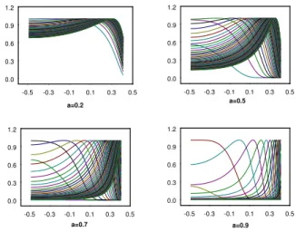
In order to simulate from the density function given in equation (19) we apply the accept reject method (see Devroye [9]), because the density is proportional to a function which has finite support (₋1₂,1₂) and which is bounded with value 1 at the maximum y∗_{, where y}∗ _{is such that} τα,β(y∗) = x. To emphasize numerical problems which arise in making inference on stable

distributions, we plot in Fig. 4 the density function of y for different values of x. Note that for all values of α _∈(0,1), high values of x make the density function spiked around the mode. Thus the basic accept method performs quite poorly. A way to improve the simulation method is to build a histogram with the rejected values and to use it as an envelope in the accept reject algorithm.

Due to the way the parameter α enters in the likelihood, the densities given in Equations (20), (21), (22) and (23) are undulating and rather concentrated, therefore as suggested by Buckle [6] and Ravishanker and Qiou [30] we introduce the following reparametrisations which give a more manageable form of the conditional posteriors of α,β and δ

vi=τα,β(yi) (24)

φi =

τα,β

xi−δ

(25) the resulting posteriors are

π(α_|β, δ, σ,x,v)_∝ α n |α₋1_|nexp ( − n X i=1 zi vi α (α−1) ) _n Y i=1 zi vi α (α−1) dτα,β dy −1 τα,β(y)=vi π(α) (26) π(β_|α, δ, σ, zi, vi) = n Y i=1 dτα,β dy −1 τα,β(y)=vi π(β) (27) π(δ_|α, β, σ, zi, vi)∝ n Y i=1 dτα,β dy −1 τα,β(y)=φi(xi−δ) π(δ) (28)

At each step of the reparametrised Gibbs sampler, the Jacobian of the transformation, dτα,β dy −1 , must be evaluated inyi =τ_α,β−1(vi). Due to the complexity of the functionτα,β, its inverse has not

an analytical expression. Therefore, following Buckle [6], the inverse transformation is determined numerically. We use the modified safeguard Newton algorithm proposed in Press et al. [28]. In order to simulate from the posteriors given in Equations (26), (27) and (28) we use Metropolis-Hastings algorithm (see Chapter??for an introduction to Monte Carlo Markov Chain methods)

Given θ(_ik−1)

(i) Generate from the proposal distribution θ∗_{i ∼}q(θi|θi(k−1))

(ii) Take: θ(_ik)= ( θ∗_i with probability ρ(θ_i(k−1), θ_i∗) θ(_ik−1) with probability 1₋ρ(θ_i(k−1), θ_i∗) where: ρ(θ(_ik−1), θ∗_i) = 1_∧ π(θ∗ i|θ−i) π(θ(k_i −1)|θ−i) q(θ(k_i −1)) q(θ∗ i) .

In order to simulate the full conditional posteriors given in Eq. (26) and (27), we use a beta distribution, _Be(a, b) as proposal. The sample generated from the beta distribution is not independent because in order to simulate the k-th value of the M.-H. chain, we pose the mean of the beta distribution to be equal to the (k₋1)-th value of the chain. In setting a and b, the parameters of the proposal distribution we distinguish the following cases

( a= α2k−1(1−αk−1)−v αk−1 v b=a1−αk−1 αk−1 when α_∈[0,1) and ( a= (αk−1−1)2(2−αk−1)−v(αk−1−1) v b=a 2−αk−1 (αk−1−1) when α_∈(1,2]

whereαk−1 is the value generated by the Metropolis-Hastings chain at step (k−1) and v is the variance of the proposal distribution. This parameters choice allows us also to avoid numerical problems related to the evaluation of the Metropolis-Hastings acceptance ratio in the presence of fat tailed and quite spiked likelihood functions.

We use a gaussian random walk proposal to simulate the full conditional posterior of the location parameter (Eq. (28)).

In order to complete the description of the hierarchical model and of the associated Gibbs sampler, we consider the following joint prior distribution

I(α)_(1,2]1 2I(β)[−1,1] 1 √ 2πb3 e− (δ−a₃₎2 2b_{3 I(δ)} (−∞,+∞) ba4 4 Γ(a4) e−bθ4 θa4+1I(θ)[0,∞) (29)

whereθ=σαα−1. We use informative priors for the location and scale parameters. Forδwe assume

a normal distribution. Note that the prior distribution of θ is the inverse gamma distribution

IG(a4, b4), which is a conjugate prior of the distribution given in equation (23). Simulations of the parameter σ can be obtained from the simulated values of θ by a simple transformation. Finally for parametersα and β we assume non informative priors.

We show the efficiency of the MCMC based Bayesian inference, running the Gibbs sampler on simulated dataset. In the following examples we discuss the numerical results and also some computational remarks related to different values of the characteristic exponent.

Example 1- (Positive α-Stable Distributions)

Fig. 5, inAppendix A, exhibits the dataset of 1,000 observations generated from the positive stable distributionS0.5(0.9,0,1). Figures 6, 7 give the results of 15,000 iterations of the Gibbs sampler relative to the characteristic exponent α, and the asymmetry parameter β, for an increasing number of simulations. Figures 8, 9 exhibit the ergodic averages. Note that convergence has been achieved after 6,000 iterations. In the first experiment we use uniform priors for α and β. We set the variance of the proposal distribution (see Eq. 46) atv= 0.0001 forα, atv= 0.0009 for

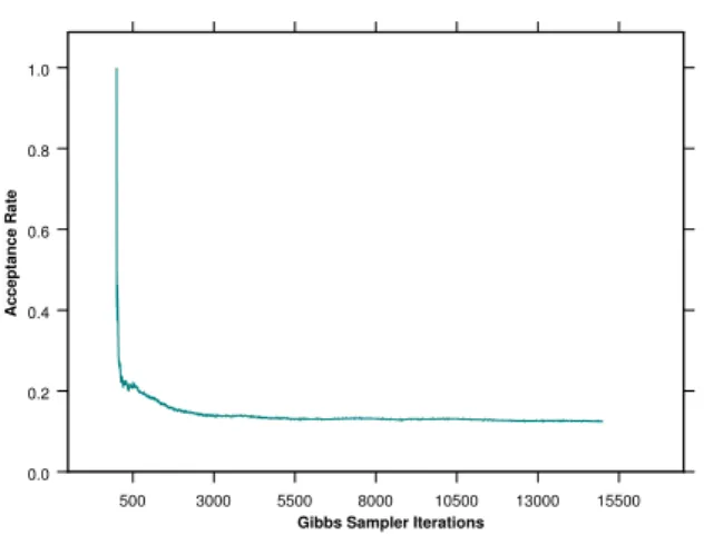
β and the starting values of the Gibbs sampler atα= 0.2 andβ = 0.5. Figures 10 and 11 exhibit the estimated acceptance rate for the M.-H. steps in the Gibbs sampler, for an increasing number of simulations. The histograms of the posteriors are depicted in figures 12 and 13. Note that through the Gibbs sample it is also possible to obtain the confidence intervals for the estimated parameters and to perform a goodness of fit test.

Example 2- (α-Stable Distributions with α >1)

Note that in the first dataset α is less than 1, therefore the moment of order less than two are infinite. In some applications like in finance, in order to give an interpretation to the result it is preferable to work at least with finite first order moments. Therefore we verify the efficiency of the Gibbs sampler also on a sample generated from a stable distribution withα _∈(1,2]. Fig. 14 in Appendix A exhibits the dataset of 1,000 values simulated from the stable distribution

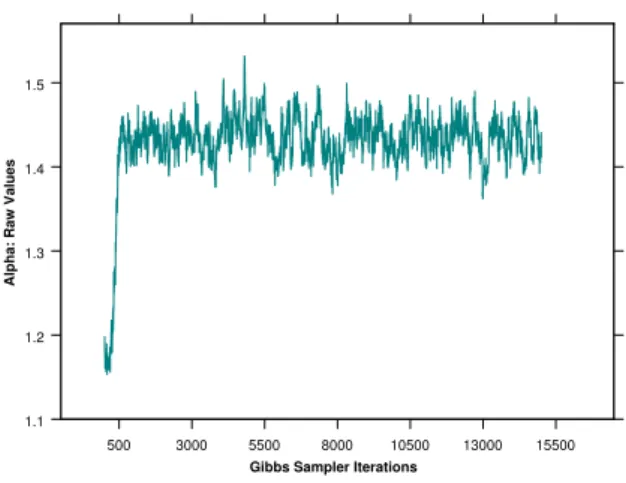
S1.5(0.9,0,1). Gibbs sampler realisations and ergodic averages are represented respectively in figures 15, 16 and in figures 17, 18. Convergence has been achieved after 6,000 iterations. In the experiment we use uniform priors for α and β and set the variance of the proposal distribution

atv= 0.0005 forα, atv= 0.0009 forβ and the starting values of the Gibbs sampler atα = 1.2 and β = 0.2. Figures 19, 20 exhibit the estimated acceptance rate, for an increasing number of simulations. Finally, posterior distributions are depicted in figures 21 and 22.

For each dataset, Table 1 summarizes the estimated parameters, the standard deviations and the estimated acceptance rates of the M.-H. steps of the Gibbs sampler. Results are obtained on a PC with Intel 1063 MHz processor, using routines implemented in C/C++. We validate the MCMC code by checking that without any data the estimated joint posterior distribution correspond to the joint prior.

Table 1: Numerical results - Ergodic Averages over 15,000 Gibbs realisations. First Dataset: S0.5(0.9,0,1)

Parameter True Value Starting Value Estimate(∗) Std.Dev. Acc. Rate

α 0.5 0.2 0.54 0.02 0.11

β 0.9 0.5 0.95 0.07 0.14

Second Dataset: S1.5(0.9,0,1)

Parameter True Value Starting Value Estimate(∗∗) Std.Dev. Acc. Rate

α 1.5 1.2 1.46 0.04 0.49

β 0.9 0.2 0.96 0.04 0.21

(*)Time (sec): 4259

(**)Time (sec): 4128

4

Bayesian Inference for Mixtures of Stable Distributions

In this section we extend the Bayesian framework, introduced in the previous section, to the mixtures of stable distributions. In many situations data may exhibit simultaneously: heavy tails, skewness, and multimodality. In time series analysis, the multimodality of the empirical distribution can also find a justification in a heterogeneous time evolution of the observed phenomena. For example, the distribution of financial time series like prices or prices volatility may have many modes because the stochastic process evolves over time following different regimes. Stable distributions allow for skewness and heavy tails, but not for multimodality. Thus a way to model these features of the data, is to introduce stable mixtures. Furthermore the use of stable mixtures is appealing also because they have normal mixtures as special case, which is a widely studied topic (see for example Stephens [38], Richardson and Green [32]). Other relevant works on the Bayesian approach to the mixture models estimation are Diebolt and Robert [10], Escobar

and West [12] and Robert [34], [33]. In Appendix C some examples of two components stable mixtures are exhibited. We simulate stable mixtures with different parameters setting, in order to understand the influence of each parameter on the shape of the mixture’s distribution.

4.1 The Missing Data Model

In the following we define a stable mixture model, while assuming to known the number of mixture components. Under a practical point of view the number of components may be detected by looking at the number of modes in the distribution or by performing a statistical test, see section 5. LetLbe the finite number of mixture components andf(x_|αl, βl, δl, σl) thel-th stable

distribution in the mixture, then the mixture model m(x_|θ, p) is

m(x_|θ, p) = L X l=1 plf(x|θl) (30) with L X l=1 pl= 1, pl≥0, l= 1, . . . , L

where θl = (αl, βl, δl, σl), l = 1, . . . , L are the parameter vector and θ = (θ1, . . . , θL) . In

the following we suppose L to be known. In order to perform Bayesian inference two steps of completion are needed. First, we adopt the same completion technique used for stable distributions. The auxiliary variable,y, is introduced in order to obtain an integral representation of the mixture distribution

m(x_|θ, p) = L X l=1 pl Z 1/2 −1/2 f(x, y_|θl)dy. (31)

The second step of completion is introduced in order to reduce the complexity problem, which arises in simulation based inference for mixtures. The completing variable (orallocation variable),

ν =_{ν1, . . . , νL} is defined as follow

νl=

(

1 if x_∼f(x, y_|θl)

0 otherwise with l= 1, . . . , L (32)

and is used to select the mixture component. The allocation variable is not observable and this missing data structure can be estimated by following a simulation based approach. Simulations from the mixture model can be performed in two step: first, simulating the allocation variable; second, simulating a mixture component conditionally on the allocation variable. The resulting demarginalized mixture model is

ν

x

b

a

L

p

L

θ

(

)

(

)

(

)

Figure 3: DAG of the Bayesian hierarchical model for inference on stable mixtures. Note that the completing variableν is not observable. Thus, two levels of completion, y andν, are needed for a stable mixture model.

m(x, ν_|θ, p) = L Y l=1 pl Z 1/2 −1/2 f(x, y_|θl)dy !νl , L X l=1 νl= 1 (33)

This completion strategy is now quite popular in Bayesian inference for mixtures (see Robert [33], Robert and Casella [35], Escobar and West [12] and Diebolt and Robert [10]). For an introduction to Monte Carlo methods in Bayesian inference from data modeled by mixture of distributions see also Neal [27] and for a discussion of the numerical and identifiability problems in mixtures inference see Richardson and Green [32], Stephens [37] and Celeux, Hurn and Robert [7].

4.2 The Bayesian Approach

The Bayesian model for inference on stable mixtures is represented through the DAG in Fig. 3. Before specifying the Bayesian model we introduce two distributions that are quite useful in Bayesian inference form mixtures: themultinomial distribution and the Dirichlet distribution.

Definition 3 (Multinomial distribution)

The random variable X= (x1, . . . , xL) has L dimensional multinomial distribution if its density

function is M(n, p1, ..., pL) = n x1. . . xL ! px1 1 ·. . .·pxLLIP xl=n (34) where PL l=1pl = 1 and pl≥0, l= 1, . . . , L.

As suggested in the literature on gaussian mixtures, in the following we assume a multinomial prior distribution for the completing variableν: V _∼fV(ν) =ML(1, p1, . . . , pL).

Definition 4 (Dirichlet distribution)

The random variable X = (x1, . . . , xL) has L dimensional Dirichlet distribution if its density

function is D(δ1, ..., δL) = Γ(δ1+...+δL) Γ(δ1)·. . .·Γ(δL) xδ1−1 1 ·. . .·xδLL−1IS(x) (35)

where δl ≥0, l= 1, . . . , L and S ={x= (x1, . . . , xL) ∈RL|Pxl = 1, xl >0 l= 1, . . . , L} is the

simplex of RL.

We assume that the parameters of the discrete part of the mixture distribution has the standard conjugate Dirichlet prior: (p1, . . . , pL) ∼ DL(δ1, . . . , δL), with hyperparameters δ1 =. . .= δL =

1

L.

Observing nindependent values, x= (x1, . . . , xn), from a stable mixture, the likelihood and the

completed likelihood are respectively

L(x,y_|θ, p) = n Y i=1 L X l=1 pl Z 1/2 −1/2 f(xi, yi|θl)dyi (36) L(x,y, ν_|θ, p) = n Y i=1 L Y l=1 (plf(xi, yi|θl))νil (37)

where y = (y1, . . . , yn) and ν = (ν1, . . . , νn) are respectively the auxiliary variable and the

allocation variable vectors andθ= (θ1, . . . , θL) andp= (p1, . . . , pL) are the mixture’s parameters

vectors. From the completed likelihood and from the priors it follows that the complete posterior distribution of the Bayesian mixture model is:

π(θ, p_|x,y, ν)_∝ n Y i=1 ( _L Y l=1 (f(xi, yi|θl))νilπ(νi) ) π(θ)π(p). (38)

Bayesian inference on the mixture parameters requires the calculation of the expected value from the posterior distribution. A closed form solution of this integration problem does not exist, thus numerical methods are needed. The introduction of auxiliary variables, that are not observable, simplifies inference for mixtures and also suggests the way to approximate numerically the problem. In fact the auxiliary variables can be replaced by simulated values and the simulated completed likelihood can be used for calculating the posterior distributions. Furthermore in order to approximate numerically the posterior means is necessary to perform simulations from the posterior distributions of the parameters and to average the simulated values.

4.3 The Gibbs Sampler for Mixtures of Stable Distributions

Gibbs sampling allows us to simulate from the posterior distribution avoiding computational difficulties due to the dimension of the parameter vector. Due to the ergodicity of the Markov chain generated by the Gibbs sampler, the choice of the initial values is arbitrary. In particular we choose to simulate them from the prior. The steps of the Gibbs sampler for a mixture model can be grouped in: simulation of the full conditional distributions and augmentation by the completing variables

(i) Simulate initial values: ν_i(0), y(0)_i , i= 1, . . . , n and p(0) respectively from

ν_i(0) _{∼ M}L(1, p1, . . . , pL) (39) y_i(0)_∼f(yi|θ, ν, xi)∝exp{1− zi τα,β(yi) α/(α−1) } zi τα,β(yi) α/(α−1) (40) p(0) _{∼ D}L(δ, . . . , δ). (41)

(ii) Simulate from the full conditional posterior distributions

π(θl|θ−l, p,x,y,v)∝ n Y i=1 {f(xi, yi|θl)pl}νil π(θl) l= 1, . . . , L (42) π(p1, . . . , pL|θ,x,y,v) =D(δ+n1(ν), . . . , δ+nL(ν)) (43)

(iii) Update the completing variables

π(yi|θ, p,x,y−i,v)∝exp ( 1₋ xi τα,β(yi) α/(α−1)) xi τα,β(yi) α/(α−1) (44) π(νi|θ, p,x,y,v−i) =ML(1, p∗1, . . . , p∗L) (45) fori= 1, . . . , n, where z= x−δ σ nl(ν) = n X i=1 νil, l= 1, . . . , L p∗_l = _PLplf(xi, yi|θl) l=1f(xi, yi|θl)pl , l= 1, . . . , L.

Steps (43) and (45) of the Gibbs sampler are proved inAppendix D. Observe that simulations from the conditional posterior distribution of Eq.(43) can be obtained by running the Gibbs sampler given in equations (20)-(23), conditionally to the value of the completing variableν. To simulate

from the Dirichlet posterior distribution given in Eq. (43), we use the algorithm proposed by Casella and Robert [35], while to draw value from the multinomial posterior distribution of Eq. (45), we use the algorithm proposed by Fishman [18].

In Examples 4.3 and 4.3, we verify the efficiency of the Gibbs sampler on some test samples simulated from stable mixtures. For each mixture’s component we assume the joint prior distribution given in equation (29). Furthermore, for the shake of simplicity, we consider

L = 2. Because of the quite irregular form of the density f(xi, yi|θl), during the MCMC based

estimation, some computational difficulties were encountered in evaluating the probability p∗ l

of each mixture’s component. Thus we introduce the following useful reparameterisation and approximation q∗_l =      eg_1(xi,yi)−g_2(xi,yi) eg_1(xi,yi)−g_2(xi,yi)₊₁ if g1> g2 or g1≤g2 1 if g1 g2 0 otherwise

wheregl(xi, yi) =log(plf(xi, yi|θl)), withl= 1,2.

Table 2: Numerical results - Ergodic Averages over 15,000 Gibbs realisations. Dataset: 0.5S1.7(0.3,1,1) + 0.5S1.3(0.5,30,1) Par. True Value Starting Value Estimate(∗) _{Std.Dev. Acc. Rate}

α1 1.7 1.9 1.66 0.09 0.32 α2 1.3 1.9 1.36 0.07 0.41 β1 0.3 0.8 0.28 0.09 0.41 β2 0.5 0.8 0.37 0.10 0.42 p1 0.5 0.4 0.52 0.02 -Dataset: 0.5S1.3(0.3,1,1) + 0.5S1.3(0.8,30,1)

Par. True Value Starting Value Estimate(∗∗) Std.Dev. Acc. Rate

α 1.3 1.7 1.25 0.08 0.23 β1 0.3 0.5 0.15 0.03 0.11 β2 0.8 0.5 0.95 0.05 0.13 p1 0.5 0.5 0.75 0.09 -p2 0.5 0.5 0.25 0.09 -(*)Time (sec):9249 (**)Time (sec):9525

Example 3- (α-Stable Mixture with varying β andα)

In this example, we apply the Gibbs sampler to a synthetic dataset of 1,000 observations generated from the stable mixture: 0.5S1.7(0.3,1,1) + 0.5S1.3(0.5,30,1). Fig. 29 inAppendix E exhibits the

dataset. In the M.-H. step of the Gibbs sampler, we set v=0.0001 for β and v=0.005 for α. Result are briefly represented in Table 4.3 and graphically described in Figg. 30-33. Note that the presence in the mixture model, of distribution with different tails behaviour, produces some problems in the convergence of the ergodic averages, due to the label switching of the observations.

Example 4- (α-Stable Mixture with constant α and varying β)

In this experiment we keep α fixed over the mixture components. First we generate 1,000 observations from the following mixture 0.5S1.3(0.3,1,1) + 0.5S1.3(0.8,30,1). Secondly we apply the Gibbs sampler for stable mixture and obtain the results given in Table 4.3. The graphical description of the results is in Figg. 35-38 ofAppendix E and exhibits a more appreciable mixing of the chain associated to the Gibbs sampler.

To conclude this section, we remark that in developing the Gibbs sampler for α-Stable mixtures and also in previous Monte Carlo experiments the number of components of the mixture is assumed to be known. Thus our research framework can be extended in order to make inference on the number of components. For example,Reversible Jump MCMC (RJMCMC) orBirth and Death MCMC (BDMCMC) could be applied in this context.

5

Application to Financial Data

Introducing two level of auxiliary variables in the stable mixture model allows us to infer all the parameters of mixture from the data. Gaussian distribution is usually assumed in modelling financial time series, but it performs poorly when data are heavy-tailed and skewed. Moreover the assumption of unimodal distribution becomes too restrictive for some financial time series. In this section, we illustrate how stable mixtures may result particularly useful in modelling different kind of financial variables and present estimates obtained with the MCMC based inferential technique proposed in the previous section.

In this example we analyse the return rate of the S&P500 composite index from 01/01/1990 to 27/01/2003. The return on the index is defined as: rt = (pt−pt−1)/pt−1. Alternatively, logarithmic returns could be used. The number of observations is 3410. Fig. 39 shows the data histogram and the best normal which is possible to estimate. The QQ-plot in Fig. 40 reveals that data are not normally distributed. We apply the Gibbs sampler for α-Stable mixtures to this dataset. The result is in Tab. 5. Parameter estimates are ergodic averages over the last 10,000 values of the 15,000 Gibbs sampler realisations. Note that index return distribution has tails heavier than Gaussian, because ˆα= 1.674.

Table 3: Parameter Estimates on S&P 500 Index daily returns. Starting Value Estimate Std.Dev. Acc. Rate

α 1.8 1.674 0.005 0.2

β 0.2 0.159 0.004 0.1

σ 0.01 0.070 0.002

-δ 0.0001 0.000091 0.0001 0.1

Example 6- (Bond Market)

Our second dataset (source: DataStream) contains daily price returns on the J.P. Morgan’s indexes concerning following countries: France, Germany, Italy, United Kingdom, USA and Japan, between 01/01/1988 and 13/01/2003. Denoting with pt the price index at time t. The

return on the index is defined as: rt = (pt−pt−1)/pt−1. Fig.41 in Appendix E exhibits jointly the histogram, the best Gaussian approximation and the density line of the returns distribution. All time series exhibit a certain degree of kurtosis and skewness. Estimation result on the J.P. Morgan Great Britain index is in Tab. 5.

Table 4: Parameter Estimates on JP Morgan - Great Britain index daily returns. Starting Value Estimate Std.Dev. Acc. Rate

α 1.5 1.95 0.004 0.2

β 0.02 0.013 0.001 0.2

σ 0.01 0.270 0.003

Example 7- (3 Months Euro-Deposits Interest Rate)

Our third dataset (source: DataStream) contains daily 3-Months Interest Rates on Euro-Deposits concerning following countries: France, Germany, Italy, United Kingdom, USA and Japan, between 01/01/1988 and 13/01/2003. Fig.43 in Appendix E exhibits jointly the histogram, the best Gaussian approximation and the density line of the returns distribution. Quite all time series of this dataset exhibit multimodality.

Estimation result on the 3-month Interest Rate for France is in Tab. 5

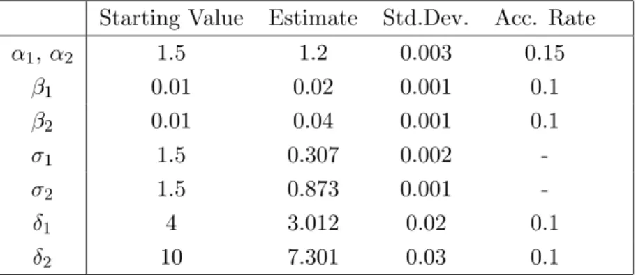
Table 5: Parameter Estimates on Interest Rates - France. Two componentsα-stable mixture. Starting Value Estimate Std.Dev. Acc. Rate

α1, α2 1.5 1.2 0.003 0.15 β1 0.01 0.02 0.001 0.1 β2 0.01 0.04 0.001 0.1 σ1 1.5 0.307 0.002 -σ2 1.5 0.873 0.001 -δ1 4 3.012 0.02 0.1 δ2 10 7.301 0.03 0.1

6

Conclusion

In this work we propose aα-Stable mixture model. As result in the literature from many empirical evidences, α-Stable distributions are particularly adapted for modelling financial variables. Moreover some financial empirical studies evidence that mixture models are needed in many cases, due to the presence of multi-modality in the asset returns distribution. We chose Bayesian inference due to the flexibility of the approach, that allows to simultaneously estimate all the parameters of the model. Furthermore we introduce a suitable reparameterisation of theα-Stable mixture in order to perform Bayesian inference. The proposed approach to α-Stable mixture models estimation is quite general and worked well in our simulation analysis, but it needs much more evaluation, with a particular attention to the case of symmetric stable mixtures. Furthermore the Bayesian approach used in this work allows to perform goodness of fit tests and also to use RJMCMC and BDMCMC techniques in order to make inference on the number of components of the mixture.

Appendix A - Bayesian Inference for Stable Distributions

Figure 4: The density function ofy for different values of x (0.04,...,0.14) and ofα (0.2,...,0.9).

0 5 10 15 20 25 30 35 40 45 50 55 60 65 70 75 80 85 90 95 0.0 0.1 0.2 0.3 0.4 0.5

Stable Distribution Histogram

500 3000 5500 8000 10500 13000 15500 0.2 0.3 0.4 0.5 0.6

Alpha: Raw Values

Gibbs Sampler Iterations

Figure 6: Gibbs sampler realisations, characteristic exponentα.

500 3000 5500 8000 10500 13000 15500 0.5 0.6 0.7 0.8 0.9 1.0

Beta: Raw Values

Gibbs Sampler Iterations

500 3000 5500 8000 10500 13000 15500 0.2 0.3 0.4 0.5 0.6

Alpha: Ergodic Averages

Gibbs Sampler Iterations

Figure 8: Gibbs sampler, ergodic averages for the characteristic exponentα.

500 3000 5500 8000 10500 13000 15500 0.5 0.6 0.7 0.8 0.9

Beta: Ergodic Average

Gibbs Sampler Iterations

500 3000 5500 8000 10500 13000 15500 0.0 0.1 0.2 0.3 0.4 0.5 Acceptance Rate

Gibbs Sampler Iterations

Figure 10: Gibbs sampler, acceptance rate of the M.-H. step, parameterα

500 3000 5500 8000 10500 13000 15500 0.0 0.2 0.4 0.6 0.8 1.0 Acceptance Rate

Gibbs Sampler Iterations

0.50 0.52 0.54 0.56 0.58 0.60 0.62 0.64 0.66 0.68 0.70

Posterior distribution of alfa

0.00 0.05 0.10 0.15

Figure 12: Gibbs sampler, histogram of the posterior π(α_|x)

0.700 0.731 0.762 0.793 0.824 0.855 0.886 0.917 0.948 0.979 1.010

Posterior distribution of beta

0.00 0.05 0.10 0.15

-5 -2 1 4 7 10 13 16 19 22 25 0.00

0.05 0.10 0.15

Stable Distribution Histogram

Figure 14: Simulated dataset, 1,000 values from S1.5(0.9,0,1).

500 3000 5500 8000 10500 13000 15500 1.1 1.2 1.3 1.4 1.5

Alpha: Raw Values

Gibbs Sampler Iterations

500 3000 5500 8000 10500 13000 15500 0.5 0.6 0.7 0.8 0.9 1.0

Beta: Raw Values

Gibbs Sampler Iterations

Figure 16: Gibbs sampler realisations, asymmetry parameterβ.

500 3000 5500 8000 10500 13000 15500 1.12

1.22 1.32 1.42

Alpha: Ergodic Average

Gibbs Sampler Iterations

500 3000 5500 8000 10500 13000 15500 0.5 0.6 0.7 0.8 0.9

Beta: Ergodic Average

Gibbs Sampler Iterations

Figure 18: Gibbs sampler, ergodic averages for the asymmetry parameterβ.

500 3000 5500 8000 10500 13000 15500 0.4

0.6 0.8 1.0

Alpha: Acceptance Rate

Gibbs Sampler Iterations

500 3000 5500 8000 10500 13000 15500 0.0 0.2 0.4 0.6 0.8 1.0

Beta: Acceptance Rate

Gibbs Sampler Iterations

Figure 20: Gibbs sampler, acceptance rate of the M.-H. step, parameter β

1.300 1.325 1.350 1.375 1.400 1.425 1.450 1.475 1.500 1.525 1.550

Posterior distribution of alfa

0.00 0.02 0.04 0.06 0.08

0.900 0.911 0.922 0.933 0.944 0.955 0.966 0.977 0.988 0.999 1.010

Posterior distribution of beta

0.0 0.1 0.2 0.3 0.4

Appendix B - Proposal Distributions for the Metropolis-Hastings

Algorithm

The shape of the stable distribution and the presence of skewness suggest us to use a Beta distribution_Be(a, b) as proposal for the Metropolis-Hastings algorithm

α_|αk−1 ∼ Be(a, b) =

1

B(a, b)α

a−1₍₁

−α)b−1I(α)(0,1). (46) We assume that the mean of the distribution is equal to the (k₋1)-th value of the M.-H. chain and set exogenously the variance equal to v. Through the parameter v it is thus possible to control the acceptance rate of the Metropolis-Hastings algorithm. When α _∈(0,1) the value of the parameters of the proposal is

( _a a+b =αk−1 ab (a+b)2_(1+a+b) =v ⇔ ( a= α2k−1(1−αk−1)−v αk−1 v b=a1−αk−1 αk−1

where αk−1 is the (k−1)-th value of the M.-H. chain and v is the variance. In addition to the previous system of equations, also the positivity constraint on the Beta’s parameters: a >0 and

b >0 must hold. Thus at each iteration of the M.-H. algorithm the following constraint must be

satisfied αk−1∈ 3₋v 2 − √ v2_{−8v+ 1} 2 , 3₋v 2 + √ v2_{−8v+ 1} 2 ! . (47)

When α_∈(1,2] we use a translated Beta distribution

α_|αk−1 ∼ Be(a, b) =

1

B(a, b)(α−1)

a−1₍₂

−α)b−1I(α)(1,2). (48) By imposing the usual constraints on the mean and the variance we obtain the values of the proposal’s parameters ( _2a+b a+b =αk−1 ab (a+b)2_(1+a+b) =v ⇔ ( a= (αk−1−1)2(2−αk−1)−v(αk−1−1) v b=a 2−αk−1 (αk−1−1)

Also in this case the positivity constraints on the Beta’s parameters must be considered. We proceed in a similar way for the proposal distribution of the skewness parameter β.

Appendix C - Mixtures of Stable Distributions

C.1 Mixtures with varying

α

Observe that in all dataset exhibited in the histograms, N=100,000 values from right skewed (β = 1) standard stables have been simulated.

-11 -6 -1 4 9 14 19 0.00 0.01 0.02 -11 -6 -1 4 9 14 0.000 0.008 0.016 0 3 6 9 12 15 0.00 0.05 0.10

Mixtures of Stable Distributions

-10 -6 -2 2 6 10 0.00 0.05 0.10 ( )1,0,1 0.5 ( )1,0,1 5 . 0 S0.2 + S0.7 0.5S0.2(1,0,1)+0.5S1.2(1,0,1) (1,0,1) 0.5 (1,0,1) 5 . 0 S1.2 + S1.7 0.5S1.2( )1,0,1+0.5S1.9( )1,0,1

Figure 23: Stables mixtures, with equally weighted components.

-11 -6 -1 4 9 14 0.00 0.01 0.02 -11 -6 -1 4 9 14 0.00 0.01 0.02 -11 -6 -1 4 9 14 0.00 0.02 0.04 0 3 6 9 12 15 0.00 0.02 0.04

Mixtures of Stable Distributions

(1,0,1) 0.8 (1,0,1) 2 . 0 S0.2 + S0.7 0.2S0.2( )1,0,1+0.8S1.2( )1,0,1 (1,0,1) 0.8 (1,0,1) 2 . 0 S1.2 + S1.7 0.2S1.2(1,0,1)+0.8S1.9(1,0,1)

C.2 Mixtures with varying

β

Simulated samples of N = 100,000 stable values are exhibited in the following histograms. In all the samples the location and the scale parameters of the mixture are: δ1 = 1, δ2 = 40,

σ1 =σ2= 7. -50 -20 10 40 70 100 130 0.00 0.02 0.04 -100 -70 -40 -10 20 50 80 0.00 0.02 0.04 -60 -35 -10 15 40 65 90 0.000 0.006 0.012 -80 -50 -20 10 40 70 100 0.000 0.008 0.016

Mixtures of Stable Distributions

(0.2,1,7) 0.5 (0.9,40,7) 5 . 0 S0.5 + S0.5 0.5S0.5(−0.2,1,7)+0.5S0.5(−0.9,40,7) (0.2,1,7) 0.5 (0.9,40,7) 5 . 0 S1.5 + S1.5 0.5S1.5(−0.2,1,7)+0.5S1.5(−0.9,40,7)

Figure 25: Stables mixtures, with equally weighted components.

-50 -28 -6 16 38 60 82 0.00 0.01 0.02 -20 1 22 43 64 85 106 0.00 0.02 0.04 -80 -55 -30 -5 20 45 70 0.00 0.02 0.04 -80 -50 -20 10 40 70 100 0.00 0.01 0.02

Mixtures of Stable Distributions

(0.2,1,7) 0.5 (0.9,40,7) 5 . 0 S0.5 + S0.5 0.5S0.5(−0.2,1,7)+0.5S0.5(−0.9,40,7) (0.2,1,7) 0.8 (0.9,40,7) 2 . 0 S1.5 + S1.5 0.2S1.5(−0.2,1,7)+0.8S1.5(−0.9,40,7)

C.3 Mixtures with varying

σ

Simulated samples of N=100,000 stable values are exhibited in the following histograms. In all the samples the location and the skewness parameters of the mixture are: δ1 = 1, δ2 = 40,

β1 =β2 = 1. -40 -18 4 26 48 70 92 0.000 0.006 0.012 0 20 40 60 80 100 120 0.000 0.015 0.030 0 30 60 90 120 150 180 0.00 0.01 0.02 -60 -28 4 36 68 100 132 0.000 0.006 0.012

Mixtures of Stable Distributions

( )1,1,5 0.5 (1,40,10) 5 . 0 S0.5 + S0.5 0.5S0.5(1,1,10)+0.5S0.5(1,40,10) ( )1,1,5 0.5 (1,40,10) 5 . 0 S1.5 + S1.5 0.5S1.5(1,1,10)+0.5S1.5(1,40,10)

Figure 27: Standard stables mixtures, with equally weighted components.

0 25 50 75 100 125 150 0.000 0.015 0.030 0 32 64 96 128 160 192 0.00 0.02 0.04 -40 -10 20 50 80 110 140 0.000 0.008 0.016 -50 -10 30 70 110 150 190 0.00 0.01 0.02

Mixtures of Stable Distributions

( )1,1,5 0.8 (1,40,10) 2 . 0 S0.5 + S0.5 0.2S0.5(1,1,10)+0.8S0.5(1,40,10) ( )1,1,5 0.8 (1,40,10) 2 . 0 S1.5 + S1.5 0.2S1.5(1,1,10)+0.8S1.5(1,40,10)

Appendix D - The Gibbs Sampler for a Stable Distributions

Mixture

Proof (Allocation Probabilities Posterior Distribution)

The posterior distribution of probabilities (p1, . . . , pL), given in Eq. (43), is a Dirichlet and is

derived in the following

π(p1, . . . , pL|θ,x,y, ν) = L(x,y, ν_|θ, p)π(θ)π(p) R L(x,y, ν_|θ, p)π(θ)π(p)dp = = Qn i=1 QL l=1(plf(xi, yi|θl))νilπ(θ)π(p) R Qn i=1 QL l=1(plf(xi, yi|θl))νilπ(θ)π(p)dp = = Qn i=1 QL l=1p νil l π(p) R Qn i=1 QL l=1p νil l Γ(δ)···Γ(δ) Γ(L δ) p δ−1 1 ,· · ·, pδL−1dp1,· · · , dpL = = Qn i=1 QL l=1pνlilπ(p) R Qn i=1 Γ(δ)···Γ(δ) Γ(L δ) QL l=1pνlil+δ−1dp1· · ·dpL = (49) = Qn i=1 QL l=1p νil l π(p) R QL l=1p Pn i=1νil+δ−1 l Γ(δ)···Γ(δ) Γ(L δ) dp1,· · · , dpL = = Γ (δ+ Pn i=1νi1)· · ·Γ (δ+ Pn i=1νiL) Γ (δ L+Pn i=1(νi1+. . .+νiL)) p Pn i=1νi1+δ−1 1 · · ·p Pn i=1νiL+δ−1 L = =_DL( n X i=1 νi1+δ, . . . , n X i=1 νiL+δ) = =_DL(n1(ν) +δ, . . . , nL(ν) +δ) where nl(ν) =Pin=1νil, withl= 1, . . . , L.

Proof (Allocation Variables Posterior Distribution)

The posterior distribution of the allocation variables given in Eq.(45) is a Multinomial and follows from

π(ν1, . . . , νn|θ, p,x,y) = L(x,y, ν_|θ, p)π(θ)π(p) R L(x,y, ν_|θ, p)π(θ)π(p)dν = = Qn i=1 n QL l=1(f(xi, yi|θl))νil QL l=1p νil l o π(θ)π(p) R Qn i=1 QL l=1(f(xi, yi|θl))νil QL l=1p νil l π(θ)π(p)dν = = n Y i=1 QL l=1(f(xi, yi|θl)pl)νil R QL l=1(f(xi, yi|θl)pl)νildνi = (50) = n Y i=1 L Y l=1 f(xi, yi|θl)pl PL l=1f(xi, yi|θl)pl !νil = = n Y i=1 ML(1, p∗1, . . . , p∗L) where p∗_l = f(xi,yi|θl)pl PL l=1f(xi,yi|θl)pl, for l= 1, . . . , L.

Appendix

E

-

Bayesian

Inference

for

Stable

Distributions

Mixtures

E.1 Mixtures with varying

α

and

β

-10 -4 2 8 14 20 26 32 38 44 50 V1 0 20 40 60 80

Figure 29: Simulated dataset, 1,000 values from 0.5S1.7(0.3,1,1) + 0.5S1.3(0.5,30,1)

3000 8000 13000 1.5 1.8 3000 8000 13000 1.4 1.8 3000 8000 13000 1.7 1.9

Alpha1: Ergodic Average

3000 8000 13000 1.5

1.9

Alpha2: Ergodic Average

Alpha1: Raw Values _{Alpha2: Raw Values}

3000 8000 13000 0.0

0.4

Beta1: Raw Value

3000 8000 13000 0.0

0.4

Beta2: Raw Value

3000 8000 13000 0.4

0.8

Beta1: Ergodic Average

3000 8000 13000 0.4

0.8

Beta2: Ergodic Average

Figure 31: Gibbs sampler realisations and ergodic averages forβ1 andβ2.

3000 8000 13000 0.41 0.52 p1 3000 8000 13000 0.41 0.52 p2 3000 8000 13000 0.40 0.45 p1 3000 8000 13000 0.48 0.54 p2

3000 8000 13000 0.1

0.3

Alpha1: Acceptance Rate

3000 8000 13000 0.5

1.0

Alpha2: Acceptance Rate

3000 8000 13000 0.5

1.0

Beta1: Acceptance Rate

3000 8000 13000 0.3

0.6

Beta2: Acceptance Rate

E.2 Mixtures with fixed

α

and varying

β

Figure 34: Simulated dataset, 1,000 values from 0.7S1.3(0.3,1,1) + 0.3S1.3(0.8,30,1)

3000 8000 13000 1.0 1.2 1.4 1.6 1.8

Alpha: Raw Values

3000 8000 13000 1.2 1.3 1.4 1.5 1.6 1.7

Alpha: Ergodic Average

3000 8000 13000 0.2

0.4

Beta1: Raw Values

3000 8000 13000 0.7

1.0

Beta2: Raw Values

3000 8000 13000 0.2

0.4

Beta1: Ergodic Average

3000 8000 13000 0.6

0.8

Beta2: Ergodic Average

Figure 36: Gibbs sampler realisations and ergodic averages forβ1 andβ2.

3000 8000 13000 0.7 1.0 p1 3000 8000 13000 0.2 0.5 p2 3000 8000 13000 0.6 0.7 p1 3000 8000 13000 0.3 0.4 p2

3000 8000 13000 0.1

0.3

Alpha: Acceptance Rate

3000 8000 13000 0.0

0.5 1.0

Beta1: Acceptance Rate

3000 8000 13000 0.01

0.12

Beta2: Acceptance Rate

E.3 Stock price indexes

S&P500 Composite Index − Daily Returns S&P Index Returns

N(s=0.0104)

Figure 39: Dataset of daily price returns

−0.035 −0.030 −0.025 −0.020 −0.015 −0.010 −0.005 0.000 0.005 0.010 0.015 0.020 0.025 0.030 0.035 −0.06 −0.04 −0.02 0.00 0.02 0.04 0.06 QQ plot

S&P Index Return × Normal

Figure 40: QQ-plot of daily price returns distribution against a normal distribution with the same mean and variance

E.4 Bond Indexes

-2 -1 0 1 2 3 1

2

JP Morgan Index - Daily Returns rJPM_GBP N(s=0.346) -1.5 -1 -.5 0 .5 1 1 2 3 4 _{rJPM_JPY} N(s=0.221) -1 -.5 0 .5 1 1 2 3 rJPM_FRF N(s=0.25) -1 -.5 0 .5 1 1.5 2 4 rJPM_BEFN(s=0.207) -1.5 -1 -.5 0 .5 1 1 2 3 4 _{rJPM_GER} N(s=0.211) -2 -1 0 1 2 1 2 3 4 _{rJPM_ITA} N(s=0.27)

Figure 41: Dataset of daily price returns

−1.0 −0.5 0.0 0.5 1.0 −2 0 2 QQ plot rJPM_GBP × Normal −0.75 −0.50 −0.25 0.00 0.25 0.50 0.75 −1 0

1 QQ plotrJPM_JPY × Normal

−0.75 −0.50 −0.25 0.00 0.25 0.50 0.75 −1 0 1 QQ plotrJPM_FRF × Normal −0.50 −0.25 0.00 0.25 0.50 0.75 −1 0 1

2 QQ plot_{rJPM_BEF × Normal}

−0.50 −0.25 0.00 0.25 0.50 0.75 −1

0

1 QQ plot_{rJPM_GER × Normal}

−0.5 0.0 0.5 1.0 −2 0 2 QQ plot rJPM_ITA × Normal

Figure 42: QQ-plots of daily price returns distribution against a normal distribution with the same mean and variance

E.5 3-Months Interest Rates

0 5 10 15 20 .05

.1 .15

Interest rate on 3 months Euro Deposit ITA3m N(s=3.64) 2 4 6 8 10 .2 .4 GER3m N(s=2.16) 0 2 4 6 8 10 .25 .5 JPY3m N(s=2.59) 2.5 5 7.5 10 .2 .4 _{USA3m N(s=1.94)} 2.5 5 7.5 10 12.5 15 .2 .4 FRF3m N(s=2.78) 2.5 5 7.5 10 12.5 15 17.5 .1 .2 UK3m N(s=3.21)

Figure 43: Dataset of daily interest rates

−5 0 5 10 15 20 0

10

20 QQ plotITA3m × Normal

−2.5 0.0 2.5 5.0 7.5 10.0 12.5 0 5 10 15 QQ plot_GER3m × Normal −7.5 −5.0 −2.5 0.0 2.5 5.0 7.5 10.0 12.5 −5 0 5 10 QQ plot JPY3m × Normal 0.0 2.5 5.0 7.5 10.0 12.5 0 5 10 QQ plot USA3m × Normal 0 5 10 15 0 10 QQ plot FRF3m × Normal 0 5 10 15 20 0 10

20 QQ plot_{UK3m × Normal}

Figure 44: QQ-plots of daily interest rates distribution against a normal distribution with the same mean and variance

References

[1] Adler R.J., Feldman R.E., Taqqu M.S. (1998),A Practical Guide to Heavy Tails: Statistical Techniques and Applications, Birkauser Ed., Boston.

[2] Barnea A., Downes D.H. (1973), A Reexamination of the Empirical Distribution of Stock Price Changes, Journal of the American Statistical Association, Vol. 68, Issue 342, pp. 348-350.

[3] Beedles W.L., Simkowitz M.A. (1980), Asymmetric Stable Distributed Security Returns,

Journal of the American Statistical Association, Vol. 75, Issue 370, pp. 306-312.

[4] Bradley B.O., Taqqu M.S. (2001), Financial Risk and Heavy Tails, Preprint, Boston University.

[5] Brennen M. (1974), On the Stability of the Distribution of the Market Component in Stock Price Changes, Journal of Financial Quantitative Analysis, Vol. 9, Issue 6, pp. 945-961.

[6] Buckle D.J. (1995), Bayesian inference for stable distribution, Journal of American Statistical Association, Vol. 90, pp. 605-613.

[7] Celeux G., Hurn M., Robert C.P. (2000), Computational and inferential difficulties with mixture posterior distributions, Journal of American Statistical Association, 95, pp. 957-979.

[8] Chambers J.M., Mallows C.L., Stuck B.W. (1976), A Method for Simulating Stable Random Variables, Journal of the American Statistical Association, Vol. 71, Issue 354, pp. 340-344.

[9] Devroye L. (1986), Nonuniform Random Variate Generation, Springer Verlag, New York. [10] Diebolt J., Robert C.P. (1994), Estimation of Finite Mixture Distributions through Bayesian Sampling, Journal of the Royal Statistical Society, Series B (Methodological), Vol. 56, Issue 2, pp. 363-375.

[11] DuMouchel W. (1973), On the Asymptotic Normality of the Maximum-Likelihood Estimate when Sampling from a Stable Distribution, Annals of Statistics, 3, pp.948-957. [12] Escobar M.D., West M. (1995), Bayesian density estimation and inference using mixtures,

[13] Fama E.F. (1965), The Behavior of Stock Market Prices, Journal of Business, 34, pp. 420-429.

[14] Fama E.F. (1965), Portfolio Analysis in a Stable Paretian Market, Management Science, B 2, pp. 409-419.

[15] Fama E.F., Roll R. (1968), Some Properties of Symmetric Stable Distributions, Journal of the American Statistical Association, 68, pp. 817-836.

[16] Fama E.F., Roll R. (1971), Parameter Estimates for Symmetric Stable Distributions,

Journal of the American Statistical Association, 66, pp. 331-338.

[17] Fielitz B.D., Rozelle J. P. (1983), Stable Distributions and the Mixtures of Distributions Hypotheses for Common Stock Returns,Journal of the American Statistical Association, Vol. 78, Issue 1983, pp. 28-36.

[18] Fishman G.S. (1996), Monte Carlo: concepts, algorithms, and applications, Springer Verlag, New York.

[19] Geman S., Geman D. (1984), Stochastic relaxation, Gibbs distributions and the Bayesian restoration of images, IEEE Transactions in Pattern Analysis and Machine Intelligence, 6, pp. 721-741.

[20] Gilks W.R., Richardson S. and Spiegelhalter D.J. (1996), Markov Chain Monte Carlo in Practice, London: Chapman & Hall.

[21] Godsill S. (1999), MCMC and EM-based methods for inference in heavy-tailed processes withα-stable innovations,Working paper, Signal Processing Group, Dep. of Engineering, University of Cambridge.

[22] Mandelbrot B., (1963), The Variation of Certain Speculatives Prices, Journal of Business,36,394-419.

[23] McLachlan G., Peel D. (2000), Finite Mixture Models, John Wiley & Sons.

[24] Meyn S.P., Tweedie R.L. (1993), Markov Chains and Stochastic Stability, Springer-Verlag, New York.

[25] Mittnik S., Rachev T., Paolella M.S. (1998), Stable Paretian modelling in finance: Some empirical and theoretical aspects. In Adler et. al., editor, A Practical Guide to Heavy Tails, Birkhauser, Boston, 1998.

[27] Neal R. M. (1991), Bayesian Mixture Modeling by Monte Carlo Simulation, Technical Report, CRG-TR-91-2, Department of Computer Science, University of Toronto.

[28] Press W., Teukolsky S., Vetterling T. and Flannery B.P. (1992), Numerical Recipes in C: The Art of Scientific Computing, Cambridge University Press, Cambridge.

[29] Qiou Z., Ravishanker N., and Dey D.K. (1999), Multivariate Survival Analysis with Positive Stable Frailties, Biometrics, vol. 55 pp. 81-88.

[30] Qiou Z., Ravishanker N. (1998), Bayesian inference for time series with infinite variance stable innovations. In Adler R., Feldman R. and Taqqu M. editors, A Practical Guide to Heavy Tails, pp. 259-282, Birkhauser, Boston, 1998.

[31] Rachev S., Mittnik S. (2000), Stable Paretian Models in Finance, John Wiley & Sons. [32] Richardson S., Green P.J. (1997), On Bayesian analysis of mixtures with an unknown

number of components, Journal of Royal Statistics Society, Ser. B, 59, pp. 731-792. [33] Robert C.P. (2001), The Bayesian Choice, 2nd ed. Springer Verlag, New York.

[34] Robert C.P. (1996), Mixtures of distributions: Inference and estimation. InMarkov Chain Monte Carlo in Practice (Eds W.R.Gilks, S.Richardson and D.J.Spiegelhalter). London: Chapman & Hall.

[35] Robert C.P. and Casella G. (1999), Monte Carlo Statistical Methods, Springer Verlag, New York.

[36] Samorodnitsky G. and Taqqu M.S. (1994), Stable Non-Gaussian Random Processes: Stochastic Models with Infinte Variance, Chambrdige University Press.

[37] Stephens M. (2000), Bayesian Analysis of Mixture Models with an Unknown Number of Components: an alternative to reverstible jump methods, Annals of Statistics, 28, pp. 40-74.

[38] Stephens M. (1997), Bayesian Methods for Mixtures of Normal Distributions,Ph.D. thesis, University of Oxford.

[39] Teichmoeller J. (1971), A Note on the Distribution of Stock Price Changes, Journal of the American Statistical Association, 66, pp. 282-284.

[40] Tierney L. (1994), Markov chains for exploring posterior distributions (with discussion),

[41] Weron R. (1996), On the Chambers-Mallows-Stuck Method for Simulating Skewed Stable Random Variables, Working Paper, Technical University of Wroclaw, Poland.

[42] Zoloratev V.M. (1966), On Representation of Stable Laws by Integrals, Selected Translations in Mathematical Statistics and Probability, 6, pp. 84-86.