Research Article A Modified Harmony Search Algorithm for Solving the Dynamic Vehicle Routing Problem with Time Windows

(1)

Research Article

A Modified Harmony Search Algorithm for Solving the Dynamic

Vehicle Routing Problem with Time Windows

Shifeng Chen, Rong Chen, and Jian Gao

Department of Information Science and Technology, Dalian Maritime University, Dalian 116026, China Correspondence should be addressed to Rong Chen; [email protected]

Received 19 April 2017; Accepted 2 November 2017; Published 28 November 2017 Academic Editor: Emiliano Tramontana

Copyright © 2017 Shifeng Chen et al. This is an open access article distributed under the Creative Commons Attribution License, which permits unrestricted use, distribution, and reproduction in any medium, provided the original work is properly cited. The Vehicle Routing Problem (VRP) is a classical combinatorial optimization problem. It is usually modelled in a static fashion; however, in practice, new requests by customers arrive after the initial workday plan is in progress. In this case, routes must be replanned dynamically. This paper investigates the Dynamic Vehicle Routing Problem with Time Windows (DVRPTW) in which customers’ requests either can be known at the beginning of working day or occur dynamically over time. We propose a hybrid heuristic algorithm that combines the harmony search (HS) algorithm and the Variable Neighbourhood Descent (VND) algorithm. It uses the HS to provide global exploration capabilities and uses the VND for its local search capability. In order to prevent premature convergence of the solution, we evaluate the population diversity by using entropy. Computational results on the Lackner benchmark problems show that the proposed algorithm is competitive with the best existing algorithms from the literature.

1. Introduction

The Vehicle Routing Problem (VRP) was first introduced in 1959 [1]. Since then, it has become a central research problem in the field of operation research and is also an important application in the areas of transportation, distribution, and logistics. The problem involves a depot, some customers, and some cargo. The cargo must be delivered from a central depot to customers at various locations using several vehicles. This is a combinatorial optimization problem in which the goal is to find an optimal solution that satisfies the service requirements, routing restrictions, and vehicle constraints.

DVRPs have been a vital research area for last 3 decades. Thanks to recent advances in information and communica-tion technologies, vehicle fleets can now be managed in real time. In this context, Dynamic Vehicle Routing Problems (DVRPs) are becoming increasingly important [2–4]. A variety of aspects is addressed by numerous approaches. Early research on DVRP can be found in Psaraftis’s work [5]. They proposed a dynamic programming approach. Bertsimas and Van Ryzin [6] considered a DVRP model with a single vehicle and no capacity restrictions where requests appear randomly. They characterized the problem by a generic mathematical model that regarded waiting time as the objective function.

Regarding DVRPTW, Chen and Xu [7] proposed a dynamic column generation algorithm for the DVRPTWs based on their notion of decision epochs over the planning horizon, which indicate the best times of the day to execute the reoptimization process. de Oliveira et al. [8] addressed the issue that arises with customers whose demands take place in real time in the DVRPTW and a capacitated fleet. Their solution was obtained through a metaheuristic approach using an ant colony system. Hong [9] also considered time windows and the fact that some requests may be urgent. This work adopted a continuous reoptimization approach and used a large neighbourhood search algorithm. When a new request arrives, it is immediately considered to be included in the current solution; therefore, it runs the large neigh-bourhood search again to obtain a new solution. de Armas and Meli´an-Batista [10] tackled a DVRPTW with several real-world constraints. Similar to Hong’s work, they also adopted a continuous reoptimization approach, but they calculated solutions using a variable neighbourhood search algorithm. In some recent surveys, Pillac et al. [11] classify routing problems from the perspective of information quality and evolution. They introduce the notion of degree of dynamism and present a comprehensive review of applications and solution methods for dynamic vehicle routing problems.

Volume 2017, Article ID 1021432, 13 pages https://doi.org/10.1155/2017/1021432

(2)

Bekta et al. [12] provide another survey in this area; they provide a deeper and more detailed analysis. Last but not least, Psaraftis et al. [13] shed more light into work in this area over more than 3 decades by developing a taxonomy of DVRP papers according to 11 criteria.

As we know, for large-scaled DVRPTW, it is very difficult to develop exact methods to solve this type of problem. The majority of the existing studies deal with the metaheuristics and intelligent optimization algorithms. Harmony Search (HS) algorithm is a metaheuristic algorithm, developed in [14]. This algorithm imitates the behaviors of musical improvisation process. The musician adjusts the resultant tones with the rest of the band, relying on his own memory in the music creation, and finally the tones reach a wonderful harmony state. Similarly, it has been successfully employed by many researchers to solve various complex problems such as university course scheduling [15, 16], nurse rostering [17], water network design [18], and the Sudoku puzzle [19]. Due to its optimization ability, the HS algorithm has also been employed as a search framework to solve VRPs. To solve the Green VRP (an extension of the classic VRP), Kawtummachai and Shohdohji [20] presented a hybrid algorithm based on the HS algorithm in which the HS is hybridized by a local improvement process. They tested the proposed algorithm with a real case from a retail company, and the results indicated that the method could be applied effectively to the case study. Moreover, Pichpibul and Kawtummachai [21] presented a modified HS algorithm for the capacitated VRP and incorporated the probabilistic Clarke-Wright savings algorithm into the harmony memory mechanism to achieve better initial solutions. Then, the roulette wheel selection procedure was employed with the harmony improvisation mechanism to improve its selection strategy. The results showed that the modified HS algorithm is competitive with the best existing algorithms. Recently, Yassen et al. [22] proposed a meta-HS algorithm (meta-HAS) to solve the VRPTW. The results of comparisons confirmed that the meta-HS produces results that are competitive with other proposed methods.

As described above, the HS algorithm has been success-fully applied to solve standard VRPs but has not been applied to solve dynamic VRPs. Solving a dynamic VRP is usually more complex than solving the corresponding standard VRP, as we should solve more than one VRP when we deal with dynamic requests. It is well-known that minimizing travel distances of standard VRPs is NP-hard in the general case, so solving dynamic VRPs with the same objective function is also a hard computational task. In this paper, we propose a Modified Harmony Search (MHS) algorithm to solve the DVRPTW. It is related to the static VRPTW, as it can be described as a routing problem in which information about the problem can change during the working day. It is a discrete-time dynamic problem and can be viewed as a series of static VRPTW problem. Therefore, the MHS algorithm we proposed includes two parts: one is the static problem optimization; we combine the basic HS algorithm with the Variable Neighbourhood Descent (VND) algorithm, with the goal of achieving the benefits of both approaches to enhance searching. The combined HSVND algorithm distinguishes

itself in three aspects: first, the encoding of harmony memory has been improved based on the characteristics of routing in VRPs. Second, this augmented HS was hybridized with an enhanced VND method to coordinate search diversifi-cation and intensifidiversifi-cation effectively. In this scheme, four neighbourhood structures were proposed. Third, in order to prevent premature convergence of the solution, we evaluate the population diversity by using entropy. The other is the dynamic customer check and insertion. Four rules were employed within the DVRPTW that address the insertion of dynamic requests into the DVRPTW. Furthermore, the MHS is verified for practical implementation by using a comparison study with other recently proposed approaches. The results show that our algorithm performs better than the compared algorithms; its average refusal rate was smallest among the three compared algorithms. Moreover, travel distances computed by our algorithm were also best in 29 out of 30 instances.

The remainder of this paper is structured as follows. The next section provides a formal mathematical model of DVRP. The notations are briefly described in Section 2. Section 3 describes the main framework and details the development of the HSVND algorithm for DVRP. The experimental setting and results are presented in Section 4. Finally, Section 5 sum-marizes the major conclusions of this article and recommends some possible directions for future research.

2. Problem Definition

The DVRPTW can be mathematically modelled by an undi-rected graph𝐺 = (𝑉, 𝐸), where𝑉 = {V₀,V₁, . . . ,V_𝑛} is the set of vertices including the depot (V₀) and the𝑛customers

(V₁, . . . ,V_𝑛), also called requests, orders, or demands and𝐸 =

{(𝑖, 𝑗) : 𝑖, 𝑗 ∈ 𝑉, 𝑖 ̸= 𝑗} is the set of edges between

each pair of vertices. Each vertexV_𝑖has several nonnegative weights associated with it, namely, a request time𝜏_𝑖, a location coordinates (𝑥_𝑖, 𝑦_𝑖), the demand𝑞_𝑖, service time𝑠_𝑖, and an earliest 𝑒_𝑖 and latest 𝑙_𝑖, possible start time for the service, which define a time window[𝑒_𝑖, 𝑙_𝑖], while[𝑒₀, 𝑙₀]is the service time range. At the same time, each edge(𝑖, 𝑗)is associated a travel time𝑡_𝑖𝑗and a travel distance𝑑_𝑖𝑗.

A total number of |𝑁| customers are to be served by fixed size fleet 𝐾 of identical vehicles, each vehicle 𝑘 has associated with a nonnegative capacity𝑄. Every customer has arrival time𝑎_𝑖and begin service time𝑏_𝑖. Particularly, the vehicle is only allowed to start the service no earlier than the earliest service time𝑒_𝑖,𝑏_𝑖 = max(𝑎_𝑖, 𝑒_𝑖). In other words, if a vehicle arrives earlier than𝑒_𝑖, it must wait until𝑒_𝑖. The customers can be divided into two groups, static customers (𝑉_𝑆) and dynamic customers (𝑉_𝐷), according to the time at which the customers made their requests. Customers in𝑉_𝑆 whose locations and demands are known at the beginning of the planning horizon (i.e., time 0), are also called priority customers because they must be serviced within the current day. The locations and demands of customers who belong to set𝑉_𝐷 will be known only at the time of the order request. These customers call in requesting on-site service over time.

The objective is to accept as many requests as possible while finding a feasible set of routes with the minimum total

(3)

travelled distance. The goal we consider here is a hierarchical approach, which is similar to the goal defined in [10]. The objective functions are considered in a lexicographic order as follows.

(i) Number of refused customers. (ii) Total travelled distance. (iii) Total number of routes.

Note that [10] included 7 objective functions: total infea-sibility (Sum of the hours that the customers’ time windows are exceeded), number of postponed services, number of extra hours (sum of hours that vehicles’ working shifts are exceeded), number of extra hours (sum of the hours that the vehicles’ working shifts are exceeded), total travelled distance, total number of routes, and time balance (difference between the longest and shortest route time made by one vehicle regarding time). They regarded the time windows as soft constraints; consequently, they needed to consider these additional objective functions. In contrast, because we regarded the time windows as hard constraints, the objective functions related to time windows could be removed.

The DVRPTW can be modelled by the following formu-las. First, we introduce three binary decision variables𝜉_𝑖𝑗𝑘,𝜒_𝑘, and𝜆_𝑖, which are defined as follows:

𝜉_𝑖𝑗𝑘 = 1 if edge (𝑖, 𝑗)is travelled by vehicle 𝑘and 0 otherwise.

𝜒_𝑘= 1 if vehicle𝑘is used and 0 otherwise.

𝜆_𝑖= 1 if the dynamic customerV_𝑖is accepted. Then the main objective can be described as in the following formula: min 𝑁 ∑ 𝑖=1 (1 − 𝜆_𝑖) (1) min ∑ (𝑖,𝑗)∈𝐸 ∑ 𝑘∈𝐾 𝑑𝑖𝑗⋅ 𝜉𝑖𝑗𝑘 ₍₂₎ min 𝐾 ∑ 𝑘=1 𝜒_𝑘 (3) s.t. ∑ 𝑖∈𝑉 𝜉_𝑖𝑗𝑘= ∑ 𝑖∈𝑉 𝜉_𝑗𝑖𝑘, 1 ≤ 𝑗 ≤ 𝑛, 𝑘 ∈ 𝐾 ₍₄₎ ∑ 𝑘∈𝐾 ∑ 𝑗∈𝑉 𝜉_𝑖𝑗𝑘= 1, 1 ≤ 𝑖 ≤ 𝑛 ₍₅₎ ∑ 𝑗∈𝑉 𝜉_0𝑗𝑘= ∑ 𝑖∈𝑉 𝜉_𝑖0𝑘= 1, 𝑘 ∈ 𝐾 ₍₆₎ ∑ 𝑖∈𝑉󸀠 ∑ 𝑗∈𝑉 𝑞_𝑖𝜉_𝑖𝑗𝑘≤ 𝑄_𝑘, 𝑘 ∈ 𝐾 ₍₇₎ 𝑎_𝑖={_{ { 𝑒₀, 𝑖 = 0 𝑏_𝑖−1+ 𝑠_𝑖+ 𝑡_{𝑖,𝑖−1}, 1 ≤ 𝑖 ≤ 𝑛 + 1 (8) 𝑏_𝑖=max{𝑎_𝑖, 𝑒_𝑖} (9) (1) 𝑆 ← 𝜙

(2) 𝑆 ←HSVND(𝑆, 𝑉_𝑆, 0) //solve static customers

(3) 𝑡 ← 0 (4)while(𝑡 < 𝑙₀)do (5) 𝐷𝑡←CheckRequests(𝑆, 𝑡) (6) 𝑆 ←HSVND(𝑆, 𝐷_𝑡, 𝑡) (7) 𝑡 ← 𝑡 + 1 (8)endwhile (9)return𝑆.

Algorithm 1: General algorithm-MHS.

𝑧_𝑖= {𝑙0, 𝑖 = 𝑛 + 1

min(𝑧_𝑖+1− 𝑡_𝑖,𝑖+1− 𝑠_𝑖, 𝑙_𝑖) , 0 ≤ 𝑖 ≤ 𝑛 (10)

𝑒_𝑖≤ 𝑏_𝑖≤ 𝑧_𝑖≤ 𝑙_𝑖 (11)

𝜉𝑖𝑗𝑘, 𝜒𝑘, 𝜆𝑖∈ {0, 1} , (12)

where𝑎_𝑖is the vehicles arrival time at the customerV_𝑖and𝑏_𝑖 is the actual start time ofV_𝑖, so𝑏_𝑖=max(𝑎_𝑖, 𝑒_𝑖)as (9) stated. In addition, for each customer𝑖, let𝑧_𝑖indicate the reverse arrival time, defined as (10).

The objective function (1) minimizes the number of refused customers, (2) aims to minimize the travel distance, and (3) minimizes the total number of routes. Eq. (4) is a flow conservation constraint: each customer𝑗must have its in-degree equal to its out-degree, which is at most one. Eq. (5) ensures that each customer𝑖 (1 ≤ 𝑖 ≤ 𝑛)must be visited by exactly one vehicle. Eq. (6) ensures that every route starts and ends the central depot. Eq. (7) specifies the capacity of each vehicle. Eq. (8)–(11) define the time windows. Finally, (12) imposes restrictions on the decision variables.

The degree of dynamism of a problem (Dod) [23] is defined to represent how many dynamic requests occur in a problem. Let𝑛_𝑠and𝑛_𝑑be the number of static and dynamic requests, respectively. Then, the Dod is described as follows:

Dod= 𝑛𝑑

𝑛_𝑠+ 𝑛_𝑑× 100%, (13)

where Dod varies between 0 and 1. When Dod is equal to 0, all the requests are known in advance (static problem), whereas when it is equal to 1, all the requests are dynamic.

3. Solution Approach

In this section, we present a metaheuristic algorithm to solve the DVRPTW. First, we introduce the framework of the heuristic algorithm to show how it can solve DVRPTWs interactively. Then, we discuss the details of the proposed harmony search-based algorithm, including its initialization, the way it improvises new solutions, and its VND-based local search method. Finally, we present some strategies used to accommodate dynamic requests.

3.1. The Framework of the General Algorithm. The general

algorithm to solve a DVRPTW interactively is summarized in Algorithm 1. First, the routes and deliveries to the static

(4)

(1)initialize all parameters: HMS, HMCR, PAR, NI,𝑆_best

(2)update the location of each vehicle in𝑆at time𝑡use eq. (15).

(3)remove the unvisited customers from𝑆and inset into𝑉.

(4)for(𝑖 = 1;𝑖 ≤HMS;𝑖++)do // HM initialization

(5) initialize a solution𝑆_𝑖randomly

(6) if(𝑓(𝑆𝑖) < 𝑓(𝑆best))then

(7) 𝑆best← 𝑆𝑖

(8) end if

(9)end for

(10)repeat

(11) improvising a new solution𝑆∗

(12) if(𝑆∗is infeasible)then

(13) repair the solution

(14) end if

(15) VND(𝑆∗)

(16) if(𝑓(𝑆∗)is better than the worst HM member)then

(17) replace the worst HM member with𝑆∗. // HM update

(18) end if

(19) if(𝑓(𝑆∗) < 𝑓(𝑆best))then

(20) 𝑆best← 𝑆∗

(21) end if

(22) compute the population entropy // entropy evaluation

(23) if(the population entropy increase or remain constant)then

(24) remove the highest frequency of harmonies

(25) re-generates new harmonies

(26) end if

(27)untila preset termination criterion is met. //checking termination criterion

(28)return𝑆_best.

Algorithm 2: HSVND(𝑆, 𝑉, 𝑡).

customers are solved by HSVND, which is our proposed harmony search-based algorithm described in Section 3.2. HSVND will return the best solution found, in which all the static customers have been inserted into routes. Conse-quently, the fleet can start to deliver goods for the customers based on the routes found in this solution. Then, dynamic customers submit requests. When a new dynamic customer request occurs, the algorithm will immediately check the feasibility of servicing the request Algorithm 3 (discussed in Section 3.3). If the request is acceptable, it then invokes the HSVND again to rearrange all the known customer requests that have not been serviced so far. Otherwise, the request will be rejected. This dynamic procedure is repeated until there are no new requests. Then, the entire solution including service for all static and dynamic customers’ requests will be returned by the general algorithm.

The following subsections discuss the HSVND algorithm and the method for inserting dynamic customer requests in more detail.

3.2. The Framework of HSVND. In this section, we describe

the core of the MHS that incorporates two known methods: the harmony search (HS) algorithm and the Variable Neigh-bourhood Descent (VND) algorithm. This hybrid algorithm, called HSVND, benefits from the strengths of both HS and VND; the HS has high global search capability while the VND excels at local search.

The HS algorithm was proposed by Geem et al. [14] based on the way musicians improvise new harmonies in

(1)Select neighbourhoods𝑁_𝑙,𝑙 = 1, . . . , 𝑙_max.

(2) 𝑙 ← 1;

(3)while𝑙 ≤ 𝑙_max

(4) Find the best solution𝑆∗in neighbourhood𝑁_𝑙

(5) if𝑓(𝑆∗) < 𝑓(𝑆)then (6) 𝑆 ← 𝑆∗ (7) 𝑙 ← 1 (8) else (9) 𝑙 ← 𝑙 + 1 (10) end if (11)end While (12)return𝑆 Algorithm 3: VND(𝑆).

memory. HS is a population-based evolutionary algorithm in which the solutions are represented by the harmonies and the population is represented by harmony memory. The HS is an iterative process that starts with a set of initial solutions stored in harmony memory (HM). Each iteration generates a new solution, and then the objective function is used to evaluate the quality of the new solution. The HS method will replace the worst solution with the new solution if the new solution is of better quality than the worst solution in HM. This process repeats until a predetermined termination criterion is met. The pseudocode of the HSVND is given in Algorithm 2.

(5)

The HSVND algorithm consists of the following six steps: initialization, evaluation, improvising a new solution from the HM, local searching by VND, updating the HM, and checking the termination criteria. After initialization, the hybrid algorithm improves solutions iteratively until a termination criterion is satisfied. The following subsections explain each step in the HSVND algorithm in detail.

3.2.1. Initialization. During initialization, the parameters for

HS are initialized first. These parameters are (i) the Harmony Memory Size (HMS), which determines the number of initial solutions in HM; (ii) Harmony Memory Consideration Rate (HMCR), which determines the rate at which values are selected from HM solutions; (iii) Pitch Adjustment Rate (PAR), which determines the rate of local improvement; and (iv) the number of improvisations (NI), which corresponds to the maximum number of iterations allowed for improving the solution. Next, the initial solution population will be generated randomly and stored in the HM. These solutions are sorted in ascending order with respect to their objective function values.

The population is also initialized. HM is represented by a matrix of three dimensions. The rows contain a set of solutions, and the columns contain the vehicles (routes) for each solution𝑆_𝑖. Each vehicle route𝑟_𝑖𝑗can be considered as a sequence of customers⟨V₀,V₁, . . . ,V_𝑛,V_𝑛+1⟩, whereV₀ and

V_𝑛+1represent the depot. In classical HS, the dimensions of each harmony in HM must be the same [14]. In our study, a harmony represents a set containing𝑚vehicles (routes). Therefore, the dimension of each harmony in HM can be different, as shown in HM= { { { { { { { { { { { { { { { { { { { { { { { { { { { 𝑆₁ 𝑆2 ... 𝑆_𝑖 ... 𝑆_HMS } } } } } } } } } } } } } } } } } } } } } } } } } } } = { { { { { { { { { { { { { { { { { { { { { { { { { { { { { { { (𝑟₁₁, 𝑟₁₂, . . . , 𝑟_1𝑗, . . . , . . . , 𝑟_1𝑚₁) (𝑟₂₁, 𝑟₂₂, . . . , 𝑟_2𝑗. . . , 𝑟_2𝑚₂) ... (𝑟_𝑖1, 𝑟_𝑖2, . . . , 𝑟_𝑖𝑗, . . . , . . . , 𝑟_𝑖𝑚_𝑖) ... (𝑟_HMS₁, 𝑟_HMS₂, . . . , 𝑟_HMS_𝑗, . . . , 𝑟_HMS_𝑚_HMS) } } } } } } } } } } } } } } } } } } } } } } } } } } } } } } } , (14)

where𝑚_𝑖is the total number of vehicles in solution𝑆_𝑖. In DVRP, a decision of waiting or moving should be made when a vehicle finishes servicing a customer. In this paper,

we introduce an Anticipatory Waiting strategy. Assume that the actual time is𝑡. Vehicle𝑘has finished serving customer

V𝑥and is ready to serve the next customerV𝑦. We allow the vehicle to wait at theV_𝑥location until𝑏_𝑦− 𝑡_𝑥,𝑦. Consequently, the vehicle will be waiting at the current location, when

𝑏_𝑦− 𝑡_𝑥,𝑦> 𝑡. (15)

Solutions in the population are constructed by generating vehicle routes iteratively. The algorithm sequentially opens routes and fills them with customers until no more customers can be inserted while still keeping the routes feasible. More precisely, the procedure chooses an unrouted customer and tries to insert it into the current route to generate a feasible route that includes the customer. This step will be repeated as long as customers can be inserted into the route without violating any constraint. When this is no longer possible, the route is closed and added to the solution𝑆and the procedure continues with the next vehicle route until all the customers have been inserted into the solution.

3.2.2. Evaluating Population Entropy. The diversity of the

harmony is set according to the population entropy, and it is defined as follows: 𝑝𝑖(𝑠𝑖) = 𝑓 (𝑠𝑖) ∑HMS_𝑖=1 𝑓 (𝑠_𝑖), 𝐸 (𝑆) = −∑HMS𝑖=1 𝑝𝑖(𝑠𝑖) ⋅ln𝑝𝑖(𝑠𝑖) ln HMS , (16)

where HMS is the harmony memory size, 𝑓(𝑠_𝑖) is the objective function value of𝑖th harmony, and𝐸(𝑥)is normal-ized population entropy. In each generation, after updating HM, the population entropy is computed. If the population entropy increase or remains constant, it would certainly have taken place in premature convergence. Then, the best harmony will retain. For the others, it counts its frequency in the HM, removes the highest frequency of harmonies, and then generates new harmonies.

3.2.3. Improvising a New Solution. A new solution 𝑆 =

(𝑟₁, 𝑟₂, . . . , 𝑟_𝑚)is improvised based on three rules: (i) random

selection, (ii) memory consideration, and (iii) pitch adjust-ment. The random selection rule allows vehicle𝑟_𝑖to choose a route from the whole search range randomly. In addition to random selection, vehicle𝑟_𝑖can take the route from previous routes for the same vehicle stored in HM such that 𝑟_𝑖 ∈

{𝑟_1𝑖, 𝑟_2𝑖, . . . , 𝑟_HMS_,𝑖}. After a new pitch (route) is generated

from memory, it is further considered to determine whether a pitch adjustment is required. Specifically, the new solution is generated as follows: first, create an empty solution𝑆; next, generate a random number𝑝in the range[0, 1]. If𝑝is less than the HMCR, choose one route from HM and add it to𝑆.

(6)

7 1 3 4 5 6 0 8 Initial route 2 (a) Shift 7 1 3 4 5 6 0 8 2 (b) Exchange 7 1 3 4 5 6 0 8 2 (c) Invert 7 1 3 4 5 6 0 8 2 (d)

Figure 1: Pitch-adjusted neighbourhood structures.

Otherwise, generate new route randomly and append it to𝑆. Specifically, new pitches (routes) are generated as follows.

𝑟𝑖 ←󳨀{_{ { rand({𝑟_1𝑖, 𝑟_2𝑖, . . . , 𝑟_HMS_,𝑖}) w.p. HMCR randomly generate w.p. (1 −HMCR) . (17)

When a new route is selected from the HM, it is adjusted at the probability PAR by a local search, where PAR ∈

[0, 1]. We produce a random number 𝑞 between 0 and 1.

If 𝑞 is smaller than the PAR, then the current route will be modified via a randomly selected neighbouring strategy. The improvisation process ends when the number of vehicles in the new solution 𝑆 is equal to the smallest one stored in HM. For DVRP, different neighbourhood structures have been used to improve the routes locally. Hence, we used three neighbourhood search methods as follows.

Shift. This operation selects a customer randomly and moves

it from its current position to a new random position in the same route. For example, in Figure 1(b), customer 2 was selected and moved after the 6th customer.

Exchange. This operation selects two customers randomly

and exchanges their positions in the same route. In Figure 1(c), the positions of customers 2 and 6 were swapped.

Invert. This operation selects two customers randomly and

inverts a subsequence between them in the same route. In Figure 1(d), edges (1, 2) and (6, 7) were deleted and edges (1,

6) and (2, 7) were linked; thus, the subsequence from 2 to 6 was inverted.

Note that any local change leading to an infeasible route will be discarded; only feasible routes are accepted. Each of neighbourhood structure is controlled by a specific PAR range as follows: 𝑟_𝑖←󳨀 { { { { { { { { { { { { { { { { { Shift 0 ≤ 𝑞 <1 3PAR Exchange 1 3PAR≤ 𝑞 < 2 3PAR Invert 2 3PAR≤ 𝑞 <PAR Nothing PAR≤ 𝑞 ≤ 1. (18)

As Figure 1 shows, the new solution 𝑆 may be infea-sible because some customers may be missed or repeated. Therefore, after a new solution is produced during the improvisation process, we must check its feasibility. A repair technique is utilized to transform an infeasible solution into a feasible solution using the following two steps: first, we identify customers who are neither scheduled nor replicated in the new solution. Then, we delete any repeated customers from the old route and, finally, either assign the missed customers to any route that can accept them or generate a new route for them.

3.2.4. The VND Method. After improvising a new solution,

we use the VND method to further optimize the solution. To make the VND method available for a DVRPTW, it is necessary to define appropriate neighbourhood structures for

(7)

0 1 2 5 6 7 8 3 4 0 0 1 2 5 6 7 8 3 4 0 (a) Swap 0 1 2 5 6 7 8 3 4 0 0 1 2 5 6 7 8 3 4 0 (b) 2-opt∗ 0 1 2 5 6 7 8 3 4 0 9 0 1 2 5 6 7 8 3 4 0 9 (c) String-exchange 0 1 2 5 6 7 3 4 0 0 1 2 5 6 7 3 4 0 (d) Relocation

Figure 2: Neighbourhood structures.

DVRPTW solutions. We propose four different neighbour-hood structures as follows.

Swap. Select one customer from a route and another customer from another route and then swap them (see Figure 2(a)).

2-Opt∗. Choose two routes and exchange the last parts of both

routes after choosing two selection points, one from each route (see Figure 2(b)).

String-Exchange. Select a subsequence of customers from one

route and another subsequence of customers from another route and exchange both subsequences (where𝑑represents the maximum length of the subsequences) (see Figure 2(c)).

Relocation. Delete one customer from one route and insert it

into another route (see Figure 2(d)).

The proposed VND method is shown in Algorithm 3, starting with the first structure 𝑁₁. In each iteration, the algorithm finds a solution𝑆∗in the current neighbourhood structure with the smallest objective function value (line

(4)). In the evaluation step, if𝑓(𝑆∗) < 𝑓(𝑆), then solution

𝑆∗ _{becomes the next incumbent solution (line}₍₆₎_{) and the} algorithm continues to use𝑁₁(line(7)); otherwise, it explores the next neighbourhood structure (line(9)). When the last structure,𝑁₄, has been applied and no further improvements are possible, the VND method is terminated and returns the final local optimal solution.

3.2.5. Updating the HM. The new solution is substituted and

added to the HM if it is better than the worst harmony solution in HM in terms of the objective function value. Otherwise, the newly created solution is rejected. Then, the HM is sorted again by objective function value.

3.2.6. Checking the Termination Criteria. The procedures of

the HS continue until a termination criterion is satisfied. We employed three termination criteria:(1)reaching the max-imum number of improvisations (NI),(2)no improvement occurred after a certain number of improvisations (CUIN), and(3)the best solution in HM reached a certain value (CBS). It will stop if one of the termination criteria is satisfied.

3.3. Inserting Dynamic Requests. Required information about

a dynamic request such as its customer location and time window is acquired when the request arrives. Moreover, at a given time point, vehicles may either be servicing a customer, waiting for a customer, or moving towards the next customer. Our DVRPTW algorithm should first determine whether requests arriving at this time point can be accepted and, if so, which vehicles and which time points can service them. The algorithm should reject requests for which no vehicle can be scheduled to service them. To decide toacceptorrejecta request, we shall discuss some insertion rules.

Rule 1 (time window constraints). Suppose customer V_ℎ

(8)

(1) 𝐷_𝑡← {dynamic customers are request in time𝑡}

(2)update the location of each vehicle in𝑆by using (15).

(3)for(each dynamic customer𝑖in𝐷_𝑡)do

//decide whether toacceptorrejectcustomer𝑖by using insertion Rules 1–4.

(4) ifit satisfies Rules 1 and 2then

(5) attempts to insert the customer𝑖into an existing route by Rule 3.

(6) if not, apply Rule 4 to split a route into two new routes

(7) attempts to inserted by Rule 3 again for each two newly routes

(8) else

(9) rejectit.

(10) end if

(11) if(reject)then

(12) add𝑖to reject pool

(13) remove𝑖from𝐷_𝑡

(14) end if

(15)end for

(16)return𝐷_𝑡

Algorithm 4: Check Requests (𝑆, 𝑡).

V_𝑘or is on the way to visit that customer based on the planned router. For the new request to be inserted into the solution, it must satisfy at least one vehicle𝑘or schedule a new vehicle that can arrive atV_ℎ before the end of the customer’s time window. The rule is expressed as follows:

𝑏_𝑘+ 𝑠_𝑘+ 𝑡_𝑘,ℎ≤ 𝑙_ℎ ∃𝑘 ∈ 𝐾 (19)

or

𝜏_ℎ+ 𝑡_0,ℎ≤ 𝑙_ℎ∧ 𝜏_ℎ+ 2 ∗ 𝑡_0,ℎ+ 𝑠_ℎ≤ 𝑙₀. (20)

Rule 2(capacity constraints). A customerV_ℎcan be inserted

into route𝑟(assume it is served by vehicle𝑘) if it does not violate vehicle𝑘’s capacity constraint. The rule to check this condition is expressed as follows:

𝑞_ℎ+ ∑

𝑖∈𝑟

𝑞_𝑖≤ 𝑄_𝑘 ∃𝑘 ∈ 𝐾. ₍₂₁₎

Rule 3(direct insert). A new customer V_ℎcan be inserted

between customersV_𝑥andV_𝑦in route𝑟if it allows the vehicle to arrive at V_ℎ before the end of its time window and also servicesV_ℎafter the beginning of its time window. The rule is expressed as follows:

𝑏_𝑥+ 𝑠_𝑥+ 𝑡_𝑥,ℎ≤ 𝑙_ℎ,

𝑧_𝑦− 𝑡_𝑦,ℎ− 𝑠_ℎ≥ 𝑒_ℎ,

𝑏ℎ≤ 𝑧ℎ.

(22)

Rule 4(split insert). This rule governs the condition when

customerV_ℎcannot be inserted at any position in route𝑟; however, if route𝑟 is split into two routes (𝑟₁ and 𝑟₂) and the customer V_ℎ can be inserted into either of these two new routes (using Rules 3 and 4), then the customer can be accepted. A route𝑟 = ⟨0, . . . ,V_𝑥,V_𝑦, . . . , 0⟩can be split into

𝑟₁ = ⟨0, . . . ,V_𝑥, 0⟩and𝑟₂= ⟨0,V_𝑦, . . . , 0⟩if

𝑧𝑦− 𝑡𝑦,0≥ 𝜏ℎ. (23)

Algorithm 4 describes how dynamic requests can be inserted in a route.

4. Experimental Results

This section shows the computational results obtained from intensive experiments using the proposed HSVND. We implemented the HSVND using the C# programming lan-guage compiled for the .NET Framework 4.5 and executed all the experiments on a PC with an IntelPentiumCPU G645 processor clocked at 2.90 GHz with 2 GB of RAM running the Windows 7 operating system.

The experiments were performed on the Lackner mark, which originated from the standard Solomon bench-mark. In this benchmark, 100 customers are distributed in a Euclidean plane over 100×100 square areas, where travel times between customers equal the corresponding distances. The benchmark is divided into six groups, named R1, R2, C1, C2, RC1, and RC2, respectively. Each group contains 8 to 12 instances, so there are 56 instances in total. To accommodate the dynamic portion of the test, each instance is associated with one of five different degrees of dynamism, 10%, 30%, 50%, 70%, and 90%, respectively. In the following experi-ments, we label each instance using the notation

“Group-Index-Dod,” where Group is the group name that instance

belongs to, Index is its index within the group (using two Arabic numerals), andDodis its dynamic degree value. For example, the label “R1-05-70” denotes the fifth instance in group R1, and that instance contains 70 dynamic customers.

4.1. Parameter Settings. This subsection investigates the

HSVND parameters HMS, HMCR, and PAR, as well as the convergence speed. We randomly selected 15 instances for these experiments. They are “C1-01-50,” “C1-05-90,” “C2-01-30,” “C2-07-10,” “R1-03-30,” “R1-09-70,” “R1-03-10,” “R2-03-50,” “R2-06-10,” “R2-09-70,” “RC1-04-50,” “RC1-06-90,” “RC2-02-70,” “RC2-03-“RC1-06-90,” and “RC2-08-30.” For each instance, 10 independent runs were carried out. Because we

(9)

Table 1: The mean results of the HSVND with different HMS values. Instance 15 20 25 30 35 40 C1-01-50 706.23 706.23 706.23 706.23 706.23 706.23 C1-05-90 286.13 285.06 285.06 285.06 285.06 286.13 C2-01-30 535.42 535.42 535.42 535.42 535.42 535.42 C2-07-10 568.77 568.77 568.77 568.77 568.77 568.77 R1-03-30 980.92 980.85 980.33 977.67 985.17 980.57 R1-03-10 1189.33 1190.39 1188.02 1194.07 1190.53 1192.57 R1-09-70 444.40 444.85 442.59 443.04 443.85 444.10 R2-03-50 632.12 623.88 629.89 619.93 620.56 625.42 R2-06-10 904.03 890.96 909.91 878.53 910.96 917.38 R2-09-70 479.90 479.28 478.23 473.05 473.93 474.35 RC1-04-50 758.43 757.28 757.12 757.40 757.51 756.25 RC1-06-90 259.43 259.43 259.43 259.43 259.43 259.43 RC2-02-70 569.12 568.58 571.81 571.81 571.81 571.81 RC2-03-90 265.61 265.61 265.61 265.61 265.61 265.61 RC2-08-30 747.95 748.86 735.77 742.39 745.45 747.59

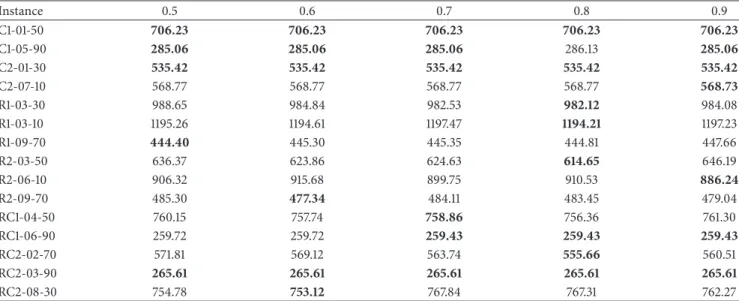
Table 2: The mean results of the HSVND with different HMCR values.

Instance 0.5 0.6 0.7 0.8 0.9 C1-01-50 706.23 706.23 706.23 706.23 706.23 C1-05-90 285.06 285.06 285.06 286.13 285.06 C2-01-30 535.42 535.42 535.42 535.42 535.42 C2-07-10 568.77 568.77 568.77 568.77 568.73 R1-03-30 988.65 984.84 982.53 982.12 984.08 R1-03-10 1195.26 1194.61 1197.47 1194.21 1197.23 R1-09-70 444.40 445.30 445.35 444.81 447.66 R2-03-50 636.37 623.86 624.63 614.65 646.19 R2-06-10 906.32 915.68 899.75 910.53 886.24 R2-09-70 485.30 477.34 484.11 483.45 479.04 RC1-04-50 760.15 757.74 758.86 756.36 761.30 RC1-06-90 259.72 259.72 259.43 259.43 259.43 RC2-02-70 571.81 569.12 563.74 555.66 560.51 RC2-03-90 265.61 265.61 265.61 265.61 265.61 RC2-08-30 754.78 753.12 767.84 767.31 762.27

split the DVRP into a series of static VRPs during the solving process, we only user the static customers at the beginning of the planning horizon (𝑡 = 0) in all experiments, and we set the termination condition of the algorithm to consider only the maximum number of improvisations (NI = 1000). Tables 1–3 show the results of the optimization of the objective functions using different settings for HMS, HMCR, and PAR.

The results in Table 1 demonstrate that the performance of the HSVND depends on the size of the HM: the larger the HMS is, the better the mean results are. Consequently, using larger values for HMS can achieve better solutions with lower objective function values. This may occur because having a larger number of solutions in the HM provides better shift patterns that are more likely to be combined into good new solutions. Therefore, HMS = 30 is chosen for all benchmark instances.

As listed in Table 2, the performance of the proposed algorithm degrades when increasing the number of random

selections when HMCR values are below 0.8. However, perturbation is necessary to bring diversity to the HM and avoid local minima. Therefore, we suggest a value of 0.8 for the HMCR based on the experimental results.

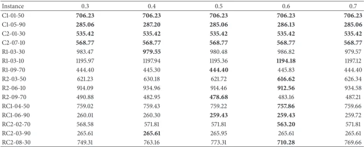
Table 3 shows that small PAR values reduce the conver-gence rate of the HSVND. Based on the experimental results, we suggest using PAR values greater than 0.6.

We also evaluated the convergence speed of the HSVND. In this experiment, we set HMS = 30, HMCR = 0.8, and PAR = 0.6 as described above. In the same way as the previous experiments, for each instance we ran the HSVND 10 times and terminated it after a maximum of NI = 1000 iterations. The maximum and average of the Continuous Unimproved Iteration Number (CUIN) and the Count of Best Solutions (CBS) are reported in Table 4, where CUIN indicates the number of iterations required to find the next local optimal solution from the current local optimal solution. During this period between the current best solution and the next one,

(10)

Table 3: The effect of the PAR on the mean function optimization. Instance 0.3 0.4 0.5 0.6 0.7 C1-01-50 706.23 706.23 706.23 706.23 706.23 C1-05-90 285.06 287.20 285.06 286.13 285.06 C2-01-30 535.42 535.42 535.42 535.42 535.42 C2-07-10 568.77 568.77 568.77 568.77 568.77 R1-03-30 983.47 979.55 980.48 986.82 979.57 R1-03-10 1195.97 1197.94 1195.36 1194.18 1197.12 R1-09-70 444.40 445.30 444.40 445.83 444.40 R2-03-50 621.23 630.18 621.72 616.62 626.34 R2-06-10 914.09 934.96 914.46 912.56 934.58 R2-09-70 490.88 482.95 478.68 483.16 487.21 RC1-04-50 759.02 759.43 759.22 757.86 759.66 RC1-06-90 260.01 260.30 259.43 259.43 259.72 RC2-02-70 568.58 571.81 571.81 563.20 571.81 RC2-03-90 265.61 265.61 265.95 265.61 265.61 RC2-08-30 749.31 763.16 773.31 710.28 769.66

Table 4: The maximum and average of CUIN and CBS.

Instance CUIN CBS

Max Avg. Max Avg.

C1-01-50 509 92.37 20 6.92 C1-05-90 911 42.95 17 2.02 C2-01-30 101 12.31 1 1.00 C2-07-10 131 24.66 30 7.09 R1-03-30 662 51.77 1 1.00 R1-03-10 611 75.46 1 1.00 R1-09-70 356 34.12 30 6.26 R2-03-50 152 23.45 1 1.00 R2-06-10 560 118.37 1 1.00 R2-09-70 563 40.15 1 1.00 RC1-04-50 713 126.00 1 1.00 RC1-06-90 71 30.63 1 1.00 RC2-02-70 152 19.34 1 1.00 RC2-03-90 49 21.30 1 1.00 RC2-08-30 815 148.10 1 1.00

CBS is defined as the number of solutions found that have the same objective value as the current best solution.

From Table 4, it can be seen that, on average, the HSVND requires at least 13 iterations to find a new local optimal solution, while, at most, it requires 150 iterations. During the search, it finds at least one solution and, at most, finds 7 solutions with the same objective value. Consequently, we set the other termination conditions as follows: CUIN = 200 and CBS = 10.

4.2. Comparison with Existing Algorithms. To assess the

performance of the proposed HSVND algorithm, we ran the algorithm on the Lackner benchmark instances and compared it with two existing methods: ILNS [9] and GVNS [10]. Comparisons were made concerning these algorithms

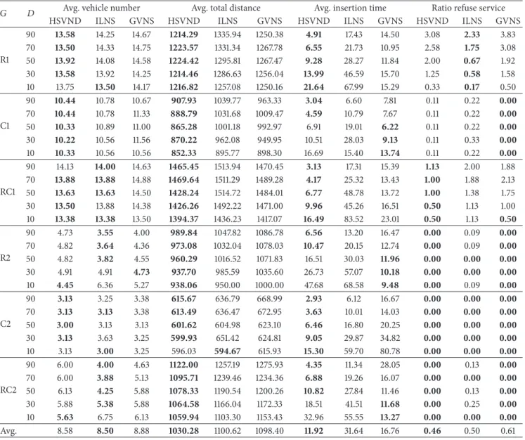
based on the ratios of refused service, the number of vehicles required, and the total distance travelled. To collect the experimental data, ten separate runs were performed for each instance and for each degree of dynamism from the Lackner benchmark. We recorded the best execution from the ten runs and calculated average values for each group. Items in boldface text in these tables indicate matches with the current best-known solution. We set the HS parameters as follows: HMS = 30, HMCR = 0.8, PAR = 0.6, NI = 1000, CUIN = 200, and CBS = 10. Table 5 lists the comparison results, where the first column indicates the group of instances (𝐺), the second column shows the degrees of dynamism (𝐷), and the other columns show the average number of vehicles, average total distance, average insertion time, and the refusal ratio, respectively. The last two rows of this table list the overall

(11)

Table 5: Comparison of the experimental results of the proposed method with other methods.

𝐺 𝐷 Avg. vehicle number Avg. total distance Avg. insertion time Ratio refuse service

HSVND ILNS GVNS HSVND ILNS GVNS HSVND ILNS GVNS HSVND ILNS GVNS

R1 90 13.58 14.25 14.67 1214.29 1335.94 1250.38 4.91 17.43 14.50 3.08 2.33 3.83 70 13.50 14.33 14.75 1223.57 1331.34 1267.78 6.55 21.73 10.95 2.58 1.75 3.08 50 13.92 14.08 14.58 1224.42 1295.81 1267.47 9.28 28.27 11.84 2.00 0.67 1.92 30 13.58 13.92 14.25 1214.46 1286.63 1256.04 13.99 46.59 15.70 1.25 0.58 1.58 10 13.75 13.50 14.17 1216.82 1257.08 1250.16 21.64 67.99 15.29 0.33 0.17 0.50 C1 90 10.44 10.78 10.67 907.93 1039.77 963.33 3.04 6.60 7.81 0.11 0.22 0.00 70 10.44 10.78 11.33 888.79 1031.68 1009.47 4.59 10.79 7.67 0.11 0.22 0.00 50 10.33 10.89 11.00 865.28 1001.18 992.97 6.91 19.01 6.22 0.11 0.22 0.00 30 10.22 10.56 11.56 870.22 962.08 949.95 10.51 28.03 9.13 0.11 0.33 0.00 10 10.33 10.56 10.56 852.33 895.77 898.30 16.69 15.40 13.74 0.11 0.22 0.00 RC1 90 14.13 14.00 14.63 1465.45 1513.94 1470.45 3.13 17.31 15.39 1.13 2.00 1.88 70 13.88 13.88 14.88 1469.64 1511.29 1489.28 4.17 25.32 13.43 1.00 1.88 2.13 50 13.63 13.63 14.50 1428.24 1514.72 1484.01 6.77 48.78 13.72 1.00 1.38 1.75 30 13.50 13.88 14.38 1426.26 1492.22 1471.00 9.96 45.26 16.51 0.50 1.13 1.00 10 13.38 13.38 13.50 1394.37 1436.23 1417.07 16.49 83.52 23.01 0.50 1.13 0.50 R2 90 4.73 3.55 4.00 989.84 1047.82 1086.78 6.56 13.20 16.47 0.00 0.09 0.00 70 4.82 3.64 4.36 973.08 1032.04 1078.03 10.47 20.15 12.74 0.00 0.09 0.00 50 4.82 3.82 4.55 960.29 1016.52 1071.83 16.51 30.03 11.96 0.00 0.00 0.00 30 4.91 4.91 4.73 937.70 985.59 1035.60 26.73 57.07 10.18 0.00 0.00 0.00 10 4.45 6.36 5.27 938.06 950.00 1000.00 47.68 68.58 9.48 0.00 0.09 0.00 C2 90 3.13 3.25 3.38 615.67 636.79 668.99 2.93 6.12 16.67 0.00 0.00 0.00 70 3.13 3.13 3.38 613.49 636.47 672.95 3.63 10.01 14.03 0.00 0.00 0.00 50 3.00 3.13 3.13 601.62 604.98 623.10 6.46 16.80 20.25 0.00 0.00 0.00 30 3.13 3.63 3.25 599.93 651.42 624.81 9.05 29.87 34.82 0.00 0.00 0.00 10 3.13 3.00 3.25 596.03 594.67 615.93 15.30 59.70 80.78 0.00 0.00 0.00 RC2 90 6.00 4.00 4.63 1122.00 1257.19 1275.93 4.35 11.34 28.05 0.00 0.13 0.00 70 6.00 3.88 5.13 1095.71 1239.46 1234.36 6.88 19.26 16.07 0.00 0.00 0.00 50 6.13 4.25 5.88 1078.33 1190.54 1200.26 10.82 27.84 11.46 0.00 0.13 0.00 30 5.88 5.38 5.88 1064.58 1166.04 1172.33 18.51 41.51 11.68 0.00 0.25 0.00 10 5.63 6.75 6.13 1059.94 1103.30 1153.43 32.96 55.55 13.27 0.00 0.00 0.00 Avg. 8.58 8.50 8.88 1030.28 1100.62 1098.40 11.92 31.64 16.76 0.46 0.50 0.61

average results obtained by the different methods and the characteristics of the computers on which the algorithms were executed.

As shown in Table 5, HSVND outperforms other meth-ods on average. First, HSVND obtains the smallest average refusal ratio, 0.46%, whereas ILNS refused 0.50%, and GVNS refused 0.61%. Both HSVND and GVNS were able to service all requests for groups R2, C2, and RC2; consequently, they obtained the same refusal ratio (i.e., 0.00%). HSVND performed better than GVNS for groups R1 and RC1 with respect to the refusal ratio while GVNS performed best for the C1 group. On average, ILNS achieves a better refusal ratio than GVNS. The average number of vehicles required by our algorithm is lower than that of GVNS but slightly larger than that of ILNS. The average number of vehicles is 8.58, 8.50, and 8.88 for HSVND, ILNS, and GVNS, respectively. However, HSVND revealed good performance in finding short distances; its average distance was 1030.28, while the average distances of ILNS and GVNS were 1100.62 and

1098.40, respectively. Note that HSVND was the best at optimizing travel distances among the three algorithms for all groups. Overall average insertion time also indicates that our proposed algorithm improves on the others; however, note that the computational environments under which the algorithms were executed are different.

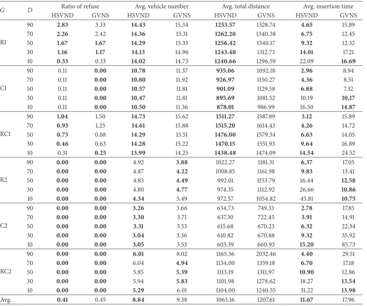
Similar to the evaluation performed for GVNS, we also calculated the average performance of 10 executions for each customer and compared that with GVNS, as shown in Table 6. HSVND improved on GVNS in terms of the avg. total distance in all cases. There are 7 types, and HSVND outperformed GVNS completely on refusal ratio, avg. number of vehicles, and avg. total distance. When the refusal ratio remains constant, there are 10 types for which HSVND can find a better solution than GVNS.

Overall, our results demonstrate that HS achieved good results compared with the existing methods as our algorithm has the ability to strike a good balance between diversification and intensification for the DVRPTWs.

(12)

Table 6: The average performance comparison of HSVND and GVNS.

𝐺 𝐷 Ratio of refuse Avg. vehicle number Avg. total distance Avg. insertion time

HSVND GVNS HSVND GVNS HSVND GVNS HSVND GVNS R1 90 2.83 3.33 14.43 15.34 1253.57 1328.74 4.65 15.89 70 2.26 2.42 14.36 15.31 1262.20 1340.38 6.75 12.45 50 1.67 1.67 14.29 15.33 1256.42 1340.17 9.32 12.32 30 1.16 1.17 14.13 14.96 1243.40 1312.73 14.01 17.21 10 0.33 0.33 14.02 14.73 1240.66 1296.59 22.09 16.69 C1 90 0.11 0.00 10.78 11.37 935.06 1092.18 2.96 8.94 70 0.11 0.00 10.80 11.92 926.97 1150.27 4.36 8.51 50 0.11 0.00 10.57 11.81 901.09 1129.58 6.88 7.32 30 0.11 0.00 10.47 11.81 895.69 1081.52 10.19 10.17 10 0.11 0.00 10.50 11.36 878.01 986.99 16.50 14.87 RC1 90 1.04 1.50 14.73 15.62 1511.27 1587.89 3.12 15.89 70 0.93 1.25 14.61 15.88 1515.20 1614.43 4.26 14.72 50 0.73 0.88 14.29 15.51 1476.00 1579.34 6.63 14.05 30 0.46 0.63 14.28 15.22 1470.15 1551.93 9.64 16.89 10 0.31 0.25 13.99 14.25 1438.48 1474.09 14.54 24.52 R2 90 0.00 0.00 4.92 3.88 1022.27 1181.31 6.37 17.05 70 0.00 0.00 4.87 4.22 1008.85 1161.98 9.83 13.41 50 0.00 0.00 4.83 4.49 992.01 1153.79 16.44 12.58 30 0.00 0.00 4.80 4.77 974.35 1112.92 26.66 10.86 10 0.00 0.00 4.34 5.49 972.57 1054.82 45.81 10.75 C2 90 0.00 0.00 3.26 3.66 634.73 749.33 2.78 17.85 70 0.00 0.00 3.30 3.71 637.30 722.45 3.91 14.91 50 0.00 0.00 3.31 3.53 615.68 670.23 6.32 22.34 30 0.00 0.00 3.04 3.36 610.82 670.88 9.32 35.92 10 0.00 0.00 3.05 3.53 603.39 660.93 15.20 85.73 RC2 90 0.00 0.00 6.01 8.02 1165.36 2032.46 4.40 29.51 70 0.00 0.00 6.04 4.94 1134.00 1359.18 6.70 17.18 50 0.00 0.00 5.85 5.39 1113.19 1311.97 10.90 12.86 30 0.00 0.00 5.94 5.83 1101.98 1278.62 18.27 13.54 10 0.00 0.00 5.29 6.01 1104.00 1240.55 31.22 13.98 Avg. 0.41 0.45 8.84 9.38 1063.16 1207.61 11.67 17.96

5. Conclusions

In this paper, we have proposed a Modified Harmony Search for DVRPTW, called MHS, which is based on HS algorithm. First of all, the encoding of harmony memory has been improved based on the characteristics of routing in VRPs. Secondly, in order to provide an effective balance between the global diversification and local intensification, an enhanced basic Variable Neighbourhood Descent (VND) is incorporated into the iterative HS. Thirdly, improvisation of a new harmony has also been improved. In this procedure, in order to prevent premature convergence of the solution, we evaluate the population diversity by using entropy. Finally, when dynamic requests arrive, five rules were employed within the DVRPTW that address the insertion of dynamic requests into the DVRPTW. In order to verify the efficiency of our approach, we carried out some numerical experiments by using standard benchmarks. Results are analyzed intensively

by comparing with recently proposed algorithms. The com-parison results show that the proposed MHS algorithm can obtain better solutions than other existing algorithms. There are several interesting future research subjects to explore. One of them can be adapting the MHS heuristic for solving other dynamic vehicle problems. Another prospective research may focus on extending the DVRPTW by introducing some realistic aspects and constraints.

Conflicts of Interest

The authors declare no conflicts of interest.

Acknowledgments

This research was partly supported by the National Natural Science Foundation of China (no. 61402070, no. 61672122,

(13)

and no. 61602077), the Natural Science Foundation of Liaon-ing Province of China (no. 2015020023), the Educational Commission of Liaoning Province of China (no. L2015060), and the Fundamental Research Funds for the Central Uni-versities (no. 3132016348, no. 3132017125). This support is gratefully acknowledged.

References

[1] G. B. Dantzig and J. H. Ramser, “The truck dispatching problem,”Management Science, vol. 6, no. 1, pp. 80–91, 1959. [2] A. Goel and V. Gruhn, “Solving a Dynamic Real-Life Vehicle

Routing Problem,” inOperations Research Proceedings, Oper-ations Research Proceedings, pp. 367–372, Springer, Berlin, Heidelberg, 2006.

[3] A. Larsen, O. B. Madsen, and M. M. Solomon, “Classification of Dynamic Vehicle Routing Systems,” inDynamic Fleet Manage-ment, Operations Research/Computer Science Interfaces Series, pp. 19–40, Springer, Boston, MA, USA, 2007.

[4] V. Pillac, C. Gu´eret, and A. Medaglia, Dynamic vehicle routing problems: state of the art and prospects 5-6, Universidad de los Andes, Bogot´a, Colombia, 2010.

[5] H. N. Psaraftis, “Dynamic programming solution to the single vehicle many-to-many immediate request dial-a-ride problem,” Transportation Science, vol. 14, no. 2, pp. 130–154, 1980. [6] D. J. Bertsimas and G. Van Ryzin, “A stochastic and dynamic

vehicle routing problem in the Euclidean plane,”Operations Research, vol. 39, pp. 601–615, 1991.

[7] Z.-L. Chen and H. Xu, “Dynamic column generation for dynamic vehicle routing with time windows,”Transportation Science, vol. 40, no. 1, pp. 74–88, 2006.

[8] S. M. de Oliveira, S. R. de Souza, and M. A. L. Silva, “A solution of dynamic vehicle routing problem with time window via ant colony system metaheuristic,” inProceedings of the 10th Brazilian Symposium on Neural Networks, SBRN ’08, pp. 21–26, Brazil, October 2008.

[9] L. Hong, “An improved LNS algorithm for real-time vehicle routing problem with time windows,”Computers & Operations Research, vol. 39, no. 2, pp. 151–163, 2012.

[10] J. de Armas and B. Meli´an-Batista, “Variable neighborhood search for a dynamic rich vehicle routing problem with time windows,”Computers & Industrial Engineering, vol. 85, pp. 120– 131, 2015.

[11] V. Pillac, M. Gendreau, C. Gu´eret, and A. L. Medaglia, “A review of dynamic vehicle routing problems,”European Journal of Operational Research, vol. 225, no. 1, pp. 1–11, 2013.

[12] T. Bekta, P. P. Repoussis, and C. D. Tarantilis, Dynamic Vehicle Routing Problems, 2014.

[13] H. N. Psaraftis, M. Wen, and C. A. Kontovas, “Dynamic vehicle routing problems: Three decades and counting,”Networks, vol. 67, no. 1, pp. 3–31, 2016.

[14] Z. W. Geem, J. H. Kim, and G. V. Loganathan, “A new heuristic optimization algorithm: harmony search,”Simulation, vol. 76, no. 2, pp. 60–68, 2001.

[15] M. A. Al-Betar and A. T. Khader, “A harmony search algo-rithm for university course timetabling,”Annals of Operations Research, vol. 194, pp. 3–31, 2012.

[16] M. A. Al-Betar, A. T. Khader, and M. Zaman, “University course timetabling using a hybrid harmony search metaheuristic algo-rithm,”IEEE Transactions on Systems, Man, and Cybernetics,

Part C: Applications and Reviews, vol. 42, no. 5, pp. 664–681, 2012.

[17] M. Hadwan, M. Ayob, N. R. Sabar, and R. Qu, “A harmony search algorithm for nurse rostering problems,” Information Sciences, vol. 233, pp. 126–140, 2013.

[18] Z. W. Geem, “Particle-swarm harmony search for water net-work design,”Engineering Optimization, vol. 41, no. 4, pp. 297– 311, 2009.

[19] Z. Geem, “Harmony Search Algorithm for Solving Sudoku,” in Knowledge-Based Intelligent Information and Engineering Systems, B. Apolloni, R. J. Howlett, and L. Jain, Eds., vol. 4692, pp. 371–378, Springer, Berlin, Germany, 2007.

[20] R. Kawtummachai and T. Shohdohji, “A Hybrid Harmony Search (HHS) algorithm for a Green Vehicle Routing Problem (GVRP),” in Proceedings of the 4th International Conference on Engineering Optimization, pp. 573–578, CRC Press, Lisbon, Portugal, 2000.

[21] T. Pichpibul and R. Kawtummachai, “Modified harmony search algorithm for the capacitated vehicle routing problem,” in Proceedings of the International MultiConference of Engineers and Computer Scientists, IMECS ’13, pp. 1094–1099, Hong Kong, China, 2013.

[22] E. T. Yassen, M. Ayob, M. Z. A. Nazri, and N. R. Sabar, “Meta-harmony search algorithm for the vehicle routing problem with time windows,”Information Sciences, vol. 325, pp. 140–158, 2015. [23] K. Lund, O. Madsen, and J. Rygaard, “Vehicle routing problems with varying degrees of dynamism,” Tech. Rep., IMM Institute of Mathematical Modelling. Technical University of Denmark, Lyngby, Denmark, 1996.

(14)

Submit your manuscripts at

https://www.hindawi.com

Computer Games Technology

International Journal of

Hindawi Publishing Corporation

http://www.hindawi.com Volume 2014

http://www.hindawi.com Volume 2014 Distributed Sensor Networks International Journal of Advances in

Fuzzy

Systems

Reconfigurable Computing

Applied

Computational

Intelligence and Soft

Computing

Advances in

Artificial

Intelligence

Hindawi Publishing Corporation http://www.hindawi.com Volume 2014 Advances in Software Engineering

Electrical and Computer Engineering Journal of -RXUQDORI &RPSXWHU1HWZRUNV DQG&RPPXQLFDWLRQV +LQGDZL3XEOLVKLQJ&RUSRUDWLRQ KWWSZZZKLQGDZLFRP 9ROXPH Hindawi Publishing Corporation

http://www.hindawi.com Volume 2014