Dual objective oil and gas field development project optimization of stochastic time cost tradeoff problems

(1)

Geo-Energy Research

www.astp-agr.com

Original article

Dual objective oil and gas field development project

optimization of stochastic time cost tradeoff problems

David A

.

Wood

∗

DWA Energy Limited, Lincoln, United Kingdom

(Received January 5, 2018; revised January 9, 2018; accepted January 9, 2018; available online January 16, 2018)

Citation:

Wood, D.A. Dual objective oil and gas field development project optimization of stochastic time cost tradeoff problems. Advances in Geo-Energy Research, 2018, 2(1): 14-33, doi:

10.26804/ager.2018.01.02.

Corresponding author:

*E-mail: [email protected]

Keywords:

Stochastic project time-cost tradeoff problems TCTP

dual-objective nondominated sorting optimization

memetic optimization algorithm with chaotic sampling

metaheuristic profiling pareto frontier

oil/gas project schedule-cost uncertainty model

Abstract:

Conducting stochastic-time-cost-tradeoff-problem (STCTP) analysis beneficially extends the scope of discrete project duration-cost analysis for oil and gas field development projects. STCTP can be particularly insightful when using a dual-objective optimization approach to locate minimum-total-project-cost solutions, and to additionally derive a Pareto frontier of non-dominated-total-project-cost solutions across a wide range of potential project durations. For STCTP project-work-item durations and costs are expressed as probability distributions and sampled with random numbers (0, 1). By controlling the fractional numbers used to sample the work-item cost distributions by formulas linked to the random numbers used to sample the work-item duration distribution, a wide range of complex time-cost relationships are readily applied. The memetic algorithm developed for constrained STCTP involves ten metaheuristics configured to focus partly on local exploitation and partly on exploration of the feasible solution space. This dual focus effectively delivers the dual objective of: 1) locating the global minimum total-project-cost solution, if it exists, or the region in the vicinity of where that solution exists; and, 2) developing a Pareto frontier. Analysis of an example project, applying eight distinct work-item time-cost relationships, demonstrates with the aid of metaheuristic profiling, that the memetic STCTP algorithm coded in Visual Basic for Applications and operated in Microsoft Excel effectively delivers on both objectives. Dynamic adjustment factors applied by some metaheuristics, derived from fat-tailed distributions adjusted by chaotic sequences, aid the efficient sampling of the feasible solution space. The metaheuristic profiles also help to fine tune the configuration of the algorithm to further enhance performance for specific work-item time-cost relationships.

1. Introduction

Providing efficient solutions to time-cost tradeoff problems is an important consideration in the planning of many oil and gas field development, facilities and improved recovery projects, while satisfying several constraints (e.g., critical path logic, activity precedence, resource availability, budget limits, quality standards etc.). The key objective is to identify an attractive/optimum time schedule that can also deliver such projects at the lowest cost while satisfying all constraints and deliverable quality standards. Zhou et al. (2013) review tech-niques used to optimize scheduling in construction projects.

Many studies propose algorithms to solve the discrete time cost tradeoff problem (DTCTP) faced by construction projects under development (e.g., Bettemir and Birgonul, 2016). The scenarios considered typically assume very specific relation-ships between cost and time of project activities, viz., as activity time is reduced by expenditure on crashing actions, the direct project cost an activity (material, labour) increases,

whereas the indirect cost (overheads) of the activity decreases. Typically, the problems evaluated are multi-modal in nature, i.e., deterministic time and cost for several alternative con-struction techniques for each activity are available for selec-tion, based upon quotes provided by different sub-contractors.

Although the multi-modal DTCTP is a common scenario and precursor to the award of engineering, procurement and construction (EPC) contracts, it is not the only scenario that needs to be considered in project planning. The uncertain-ties that exist for most work-item cost and durations at the early project planning stages justify the application of more expansive evaluations of stochastic time cost tradeoff problems (STCTP). This involves estimating the time (duration) and cost for each activity (work item) with continuous distributions rather than deterministic values. In such circumstances the uncertainties associated with duration and cost for each activity are better expressed as probability distributions. Such situa-tions typically prevail during the front-end engineering and

https://doi.org/10.26804/ager.2018.01.02.

2207-9963 cThe Author(s) 2018. Published with open access at Ausasia Science and Technology Press on behalf of the Division of Porous

(2)

design (FEED) stages and earlier pre-FEED stages of project planning. Indeed, multiple cost-time quotes from contractors for each activity, enabling a multi-modal discrete analysis, are typically not available until after a FEED study is completed. Yet, preliminary TCTP analysis can be beneficial in the FEED and pre-FEED stages of complex projects. In addition, sig-nificant uncertainty remains concerning the durations of con-tracted activities during project implementation, due to factors such as contractor performance, inflation of materials costs, weather, unplanned interruptions and change orders. A case can therefore be made for stochastic analysis during project implementation, albeit with narrower distribution ranges.

Such uncertainties expose the limitations of discrete op-timization models and justifies the use of stochastic project evaluation and review techniques (PERT) to incorporate such uncertainty in the CPM analysis. Therefore, this study proposes a stochastic STCTP approach for early-stage and implementation-stage project planning that minimizes project costs across a range of possible project durations (makespans) for different probabilistic activity time-cost relationships. It applies a newly developed memetic, nondominated, sorting optimization algorithm and monitors performance of the com-ponent metaheuristics of that algorithm with the recently-developed technique of metaheuristic profiling (Wood, 2016a; 2016b).

2. Literature review

Early work by Fulkerson (1961) and Kelley (1961) identi-fied the benefits of the critical path method (CPM) of analysis to adjust project schedules such that total project costs could be minimized. Complex relationships were recognized between project activity durations and their costs (Siemens, 1971; Reda and Carr, 1989) and the risks associated with them (Wollmer, 1985; Moselhi and Deb, 1993). In some cases, this enabled a projects schedule to be accelerated by allocating more resources (e.g., work force, equipment, materials) to certain critical activities at additional direct costs, eventually termed crash actions, constrained by available resources (Ahn and Erenguc, 1998; Gutjahr et al., 2000). The DTCTP was first formally addressed by Harvey and Patterson (1979) and Hindelang and Muth (1979), and is now generally expressed in cases where the duration of each activity in each of several modes is a discrete non-increasing function of the amount of non-renewable resource dedicated to it (Wu and Chen, 2009). DCTCP continue to be the focus of many construction-related optimization studies (e.g., De et al., 1995; Zheng, 2015; Aminbaksh and Sonmez, 2016). It is known to be a strongly NP-hard optimization problem and to become more so as additional optimization objectives are factored in (Van Peterghem and Vanhoucke, 2010; Singh and Ernst, 2011; Zhang et al., 2015), with the feasible solution space increasing exponentially as the number of project activities increases (Tavana et al., 2014). In cases where multiple objectives are sought (e.g., cost, time, quality etc.) the Pareto front approach has provided nondominated time-cost solutions over a range of feasible project schedules (Chau et al., 1997; Feng et al., 1997; Zheng et al., 2005; Vanhoucke and Debels, 2007; Iranmanesh

et al., 2008; Gomes et al., 2014; Koo et al., 2015).

Babu and Suresh (1996) recognized that project quality was also likely to be impacted by time-cost tradeoff and con-sidered time-cost-quality tradeoff as a complex continuum to be optimized. Many subsequent studies have treated time-cost-quality optimization as a discrete problem with each activity potentially executed in several modes (Kang and Myint, 1999; El-Rayes and Kandil, 2005; Tareghian and Taheri, 2006; Kim et al., 2012). Some models incorporate fuzzy logic to address the difficult-to-quantify uncertainties associated with project quality and resource utilization (Zheng and Ng, 2005; Zahraie and Tavakolan, 2009; Zang and Xing, 2010; Shahsavari Pour et al., 2012; Ahari and Niaki., 2013; Mungle et al., 2013), or apply multi-criteria decision-making techniques, such as Anal-ysis Hierarchy Method (AHP) (Pollack-Johnson and Libera-tore, 2006) or evidential reasoning (Monghaesemi et al., 2015) to assess project quality. Ke (2014) applies uncertainty theory to address non-random and non-fuzzy uncertainties in TCTP. It has been argued that the DCTCP is too narrowly specified to cover many of the real project problems encountered (Vahidi, 2013); a view shared by this author (see introduction). Also, in some projects a case can be made for focusing on profitability and optimizing project net present value (NPV) rather than costs (Zareei et al., 2014).

Methodologies applied to optimize TCTP can be broadly classified (Zhang and Xing, 2010) into heuristic methods (Fondahl, 1961; Siemens, 1971; Molehsi, 1993; Elazouni, 2009), mathematical methods (Robinson, 1975; De et al., 1995; Elmaghraby, 1995; Burns et al., 1996) including branch-and-bound methods (Rostami et al., 2014), and metaheuristic models (Feng et al., 1997; Li and Love, 1997; Zheng et al., 2004, Elbeltagi et al., 2005; Hegazy, 2011), with further exam-ples of each listed by Zhou et al. (2013). In contrast to heuris-tics, which are approximate rules-of-thumb developed using problem-specific information and tend to easily get trapped at local optima, metaheuristics are computational methods that optimize a problem by iteratively trying to improve a candidate solution with regard to a given measure of quality (Suh et al., 2011). The metaheuristic models applied to TCTP are for the most part evolutionary in nature, dominated by genetic algorithms (Chau et al., 1997; Sonmez and Bettemir, 2012), but also including ant colony (Ng and Zhang, 2008), particle swarm (Rahimi and Iranmanesh, 2008), differential evolution, simulated annealing (Rasmy et al., 2008; Anagnostopoulos and Kotsikas, 2010), harmony search (Geem, 2010), frog leaping (Eusuff et al., 2006; Elbeltagi et al., 2007; Rashtchi et al., 2012), intelligent water drops (Saif et al., 2015), etc. Some evolutionary and other algorithms are configured to also evaluate DTCTP, taking into account fuzzy quality inputs (Wood, 2017), limited resource availability (Ghoddousi et al., 2013; Afruzi et al., 2014; Rostami et al., 2014; Cheng and Tran, 2016), including renewable, nonrenewable and doubly constrained resources.

The term memetic algorithm does not have a standard definition (e.g., Moscato, 1989; Garg, 2009; Chen et al., 2011; Wood, 2016c). The definition applied here is that memetic algorithms are extensions or hybrids of metaheuristic evolu-tionary algorithms, combining multiple local and global search

(3)

components, which may not all be evolutionary in design, thereby increasing their learning capability, flexibility and efficiency in searching feasible solutions spaces in comparison to metaheuristics.

All of these optimization methods are obliged to obey a projects work-item precedencies and critical path (CPM) constraints, such that an activity is unable to start until its precedence activities are completed and, on the critical path, an activity cannot start later than its latest start time without lengthening the duration of the project overall. TCTP models have applied a range of time-cost functions and relationships (Azaron, 2005; Blaszczyk and Nowak, 2009), including linear (Fulkerson, 1961; Kelley, 1961), discrete (Demeulemeester et al., 1993), non-linear, including convex (Berman, 1964; Lamberson and Hocking, 1970), concave (Falk and Horowitz, 1972), and in some cases arbitrary, stochastic (Hagstrom, 1988; Ke and Liu, 2005; Cohen et al., 2007; Ke et al., 2009) or hybrid. Linear continuous TCTP, where activity costs decrease linearly with duration, have been solved with linear programming (Baker, 1997) and by stochastic mathematical methods (Cohen et al., 2007). Some non-linear continuous TCTP, where activity costs decrease in a convex relationship with duration, have been solved with quadratic programming (Deckro et al., 1995).

Chaos is a deterministic, non-linear, bounded, unstable, dynamic behavior resembling stochastic sampling, but with infinite unstable periodic motions dependent upon defined starting positions, Chaotic sampling may be applied in either deterministic or stochastic conditions. Chaotic sampling can assist search functions in optimization algorithms (Li and Jiang, 1999; Wang et al., 2001), and has been recently applied to bat-flight, (Lin et al., 2012), frog-leaping (Rashtchi et al., 2012) and cuckoo search (Huang et al., 2016; Wood, 2016b) algorithms. Searching solution spaces with Levy flights enhances the efficiency of cuckoo search algorithms (Yang and Deb, 2009). Choatic sampling combined with Levy flight (Huang et al., 2016) or with generic fat-tailed distributions (Wood, 2016b) further enhances the efficiency of solution-space searches, and is an approach used in some of meta-heuristic components of the memetic algorithm developed for in this study.

This study evaluates a range of stochastic time-cost re-lationships for STCTP evaluations, of a scale typical for oil and gas field developments. It does so with a memetic (evolutionary) algorithm, recognizing that due to the durations of each activity (work item) being uncertain, the costs of each activity, total project duration and costs are also uncertain, limiting the scope of deterministic models. Its dual cost and time focus requires that it seeks efficient (non-dominated) time-cost solutions over a range of feasible project durations (Pareto frontier), applying budget and schedule constraints as required. In the following sections the details of the memetic algorithm are described, it is applied to an example oil and gas facilities project using eight distinct and continuous work-item time-cost relationships, and its performance is evaluated in locating optimum solutions and in defining Pareto frontiers.

3. Memetic nondominated sorting optimization

algorithm incorporating chaotic and fat-tailed

search metaheuristics

A flowchart describing the memetic algorithm applied to continuous and stochastic project time-cost optimization problems (STCTP) is included as Appendix S Fig-S1. It consists of ten integrated metaheuristics (Mh1 to Mh10), which operate collectively across multiple iterations of the algorithm to influence an evolving population of solutions in its quest for solutions better satisfying the optimization objectives.

(1) Algorithms Control Metrics

Prior to running the algorithm, it is necessary to specify the following control metrics:

• Number of iterations (M) to run in each execution of the algorithm.

• Number of solutions (N) to generate/modify in each iteration.

• Fraction ofNto consider as high-ranking sub-population for modification.

• Work item constraints: P0, P100 values for each work item time and cost distributions.

• Full project time constraints (e.g. maximum allowable

values to consider), if required.

• Which metaheuristics to run/not run. • Set tuning values for certain metaheuristics.

• Set number of total project time intervals (Q) to use to

generate the Pareto Front for total project cost.

The algorithm is configured to minimize total project costs taking into account the specified constraints. Therefore, metaheuristic 1 (Mh1) operates in the first iteration, to gen-erate a randomly selected population of N solutions. Each solution evaluated by a PERT/critical path method (CPM) logic function in order to determine total project duration taking into account parallel sequences and precedence of work items. This generates three total project value outputs for each solution evaluated: 1. Total project cost (objective function); 2. Total project duration (taking into account parallel working and work-item precedence); and, 3. Sum of the durations of all work items (ignoring parallel working and work-item precedence). The values for output 3 will be greater than the values for output 2 in projects where parallel work item sequences are involved. The N solutions are then ranked in ascending order of the total project costs for each solution in the population, assigning each a ranking from rank #1 to rank #N.

(2) Description of Ten Integrated Metaheuristics (Mh1 to Mh10)

The following metaheuristics operate from iterations 2 to

M, and the solutions modified, retained or generated are ranked in ascending order of total project cost at the end of each iteration in preparation for the actions of the next iteration. In addition to recording the lowest total project cost solution associated with each iteration, the non-dominated por-tion of the algorithm records details of the lowest total-project-cost solutions achieved by all iterations concluded so far, in each of the Q total-project-duration intervals. This enables

(4)

progress of the Pareto frontier to be monitored iteration by iteration.

Mh1 generates random population of feasible solutions (coded 1), ranks the solutions in ascending order of objective function and sets up the intervals for the project time-cost Pareto frontier recording non-dominated solutions (i.e., lowest total project costs for all solutions with total project time within a specified interval) for each Pareto-frontier interval.

Mh2 generates a subset of modified solutions (coded 2) to replace some solutions in the N−Qlower ranking solutions of the previous iteration. It uses the cumulative frequency of high-ranking solutions and roulette wheel selection to pref-erentially select some of the high-performing (Q) solutions. It then modifies some of the randomly-selected work item durations and moves them closer towards the values recorded for some of the highest-ranking solutions (e.g. rank #1 to rank #10). The adjustment factors to make these modifications are determined by selected from fat-tailed distributions adjusted by chaotic sequences (see Wood, 2016b, and Appendix S for equations). This approach enables the adjustment factors to get progressively smaller as the number of iterations increases, thereby progressively narrowing the search area of the feasible solution space.

Mh3 generates a subset of modified solutions (coded 3) derived by making minor adjustments to the twenty-best non-dominated solutions, plus one randomly-selected from the highest-ranking solutions, recorded from the previous iteration. Either one work-item duration, or several, are modified in the solutions selected. How many work-item durations are changed depends upon the number of iterations completed so far; in early iterations, up to 30% of the work-item durations are changed, whereas in later iterations, this is progressively reduced to 10% in some iterations, and just one work-item duration in others. The adjustment factors applied also vary systematically as iterations progress, with higher adjustments made in earlier iterations. The modified solutions generated replace some solutions in the N−Qlower ranking solutions of the previous iteration that have not been replaced in the current iteration.

Mh4 generates a subset of modified solutions (coded 4) derived by shifting one, randomly selected work-item duration of ranks #1 to ranks #10 solutions close to one of their constraint boundaries (also selected randomly). If the work item duration selected is already very close to its constraint boundary, then another work item is selected. The modified solutions generated replace some solutions in theN−Qlower ranking solutions of the previous iteration that have not been replaced in the current iteration.

Mh5 generates a subset of modified solutions (coded 5) derived by adjusting multiple (e.g., 30%), randomly- selected work-item durations of high-ranking solutions (e.g. beginning at ranks #12) from the previous iteration. The adjustments are made by small increments, using dynamic random sampling of adjustment factors extracted from a fat-tailed distribution adjusted by a chaotic sequence. Once half of the iterations are completed a random change to one work-item iteration is also introduced for a few of the solutions generated to widen the search. The modified solutions generated replace

some solutions in the N−Qlower ranking solutions of the previous iteration that have not been replaced in the current iteration.

Mh6 generates a subset of modified solutions (coded 6) derived by introducing small modifications to one randomly selected work-item durations of high-ranking solutions (e.g., ranks #1 to #20) from the previous iteration. The adjust-ments are made by small increadjust-ments, using dynamic random sampling of adjustment factors extracted from a fat-tailed distribution adjusted by a chaotic sequence. If the global best solution found by recent iterations shows only a small improvement, then a second randomly-selected work-item duration is also modified by similarly-generated adjustment factors. The modified solutions generated replace the existing rank #1 to rank #20 solutions of the previous iteration, with the existing rank #1 solution preserved by replacing one of the N −Q lower ranking solutions of the previous iteration that has not been replaced in the current iteration.

Mh7 generates a subset of modified solutions (coded 7) derived by replacing one randomly selected work-item dura-tions with a random viable value for selected high-ranking solutions (e.g., selected from ranks #1 to #75) from the previous iteration. The modified solutions generated replace some solutions in the N−Qlower ranking solutions of the previous iteration that have not been replaced in the current iteration.

Mh8 generates a subset of modified solutions (coded 8) derived by crossing over selected work-item duration values in solutions rank #21 to #50 of the previous iteration with lower ranking solutions from that iteration. The number of work item durations modified in this way is high (e.g.∼60%) in the early iterations, reducing (e.g.,∼30%) in later iterations. The modified solutions generated replace the existing rank #21 to rank #50 solutions of the previous iteration.

Mh9 Substitutes previous best solutions into the top ten rankings for consideration for some adjustments by the next iteration, if the objective function value for rank #1 only differs from rank #10 by a very small specified amount. This is controlled to begin operating only after a certain number of iterations are completed and/or to operate only at intermittent iterations. It can help the algorithm to escape from local optima.

Mh10 Substitutes a few low to mid-ranking solutions from the previous iteration into the top ten rankings for consider-ation for some adjustments by the current iterconsider-ation. This is controlled to begin operating only after a certain number of iterations are completed and/or to operate only at intermittent iterations. It can also help the algorithm to escape from local optima in later iterations.

Following the execution of Mh2 to Mh8 in iterations from 2 toM there areN−1new modified solutions plus the rank #1 of the previous iteration. These solutions are each evaluated by the PERT/critical path method (CPM) logic function in order to determine total project duration taking into account parallel sequences and their precedence of work items. This generates total project output values 1 to 3 for each solution. TheNsolutions are then ranked in ascending order of the total project costs for each solution in the population, assigning

(5)

each a ranking from rank #1 to rank #N. Mh9 and Mh10 are then applied to in some cases modify that ranking for consideration by the next iteration.

Metaheuristics Mh1, Mh5, Mh7, Mh8, Mh10 are more directed towards global exploration of the feasible solution space. In contrast, metaheuristics Mh2, Mh3, Mh4, Mh6 and Mh9 are more directed towards exploitation (local search) around promising feasible solutions already found, increas-ingly focusing that search as iterations progress towards the final specified number of iterations (M). Mh2 incorporates both local and global search capabilities, being more glob-ally focused in earlier iterations and becoming more locglob-ally focused as solutions converge. It is the ability to balance exploration and exploitation of continuous feasible solution spaces, and to tune various metaheuristics to achieve both, that makes memetic algorithms attractive for this purpose. For specific projects, it is likely that certain metaheuristics are more effective than others in finding the best solutions. It is possible to tune the algorithm such that ineffective metaheuristics are switched off and the number of solutions produced by effective metaheuristics expanded, if necessary.

The memetic algorithm as described and configured is highly versatile and transferrable to other problems, with the chaotic sampling techniques associated with some metaheuris-tics relevant to the sampling of various reservoir and other sub-surface uncertainties.

4. Critical path description of example project

with continuous time-cost uncertainty ranges

A project network for an example oil and gas field facilities construction project, with several parallel paths of work items with high duration and cost uncertainties, is evaluated here using the STCTP algorithm described. The high-level-work-item breakdown of the project (20 work high-level-work-items) would be underpinned in practice by a more-detailed network analysis broken down further into probably many hundreds of individ-ual activities, which would be required to plan and implement the project in detail. Optimizing at the higher level of a project in its the early planning stages is the focus of this example.

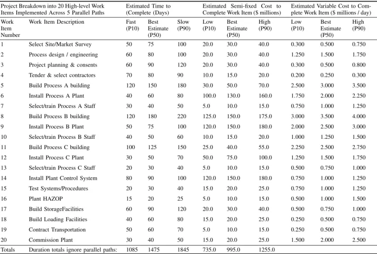
Details of the project work items uncertain durations and costs are provided in Table 1 as five distinct deterministic cases that also used to construct probability distributions for stochastic evaluations. These distributions are symmetrical about the best guess (P50-median/best guess values), but could be asymmetrical without compromising the functioning of the optimization algorithm. Assuming triangular relationships, the P0 (probability 0%/minimum) values are derived by extrap-olating the P50 and P10 (tenth percentile/ fast deterministic case) values, whereas the P100 (probability 100%/maximum) values are derived by extrapolating the P50 and P90 (ninetieth percentile/slow deterministic case) values (Table 1).

In the construction industry, it is common to distinguish two distinct cost components: direct and indirect. The direct costs associated with completing the work item (including day-rate labour and equipment costs, and are typically assumed to increase in some ways, due to greater resource deployments, as work item duration is reduced. The indirect costs are various

overhead costs incurred on a day-rate basis that increase in proportion to the time taken to complete the work item. This type of cost distinction is used for projects across all industries. A more generic approach to project time-cost relationships is to consider two alternative cost components for stochastic project work-item cost analysis, each of which can be related to work item duration in various ways. Hence, the use here of the components semi-fixed costs and variable costs (Table 1). The semi-fixed costs are those quoted costs for plant, equipment and resources that may depend or not on the time taken to complete the work item according to various relationships, but are still uncertain with the ability to vary across the P0 to P100 range. The variable costs are those that vary on a day-rate basis (including some labour and overhead costs) and increase in proportion to the time taken to complete the work item. The day rates of the variable costs are also uncertain with the ability to vary across the P0 to P100 range, but are calculated by multiplying day rates by the number of days taken to complete the work item. It is the semi-fixed and variable cost distributions of Table 1 that are related to the work item durations using various relationships that are used here to evaluate STCTP.

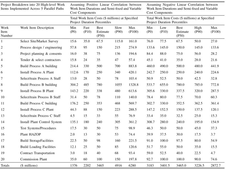
For work item time-cost distribution interactions in the stochastic model it is possible, and sometimes appropriate, to consider various relationships (positive, negative, non-linear and complex, e.g. segmental) between the duration and either of the two cost components for each work item, or between the two cost components. Table 2 lists the total work item cost (semifixed plus variable multiplied by duration) relationships for the five deterministic cases assuming positive and negative linear correlations between work-item durations and the two components of costs. In the positive linear correlation case P0, P10, P50, P90 and P100 duration cases are matched with the P0, P10, P50, P90 and P100 cases of each cost component. In the negative linear correlation case P0, P10, P50, P90 and P100 duration cases are matched with the P100, P90, P50, P10 and P0 cases of each cost component. Comparing the two sets of total work-item and full project cost values generated, highlights the significance of the time to cost distribution re-lationships in projects. Total project costs could vary between US$1376 million and US$6280 million depending upon the cases and time-cost relationships considered. It is also clear that the relationship between the total project costs of five cases for the negative linear work-item time-cost relationships (Table 5) are far from linear.

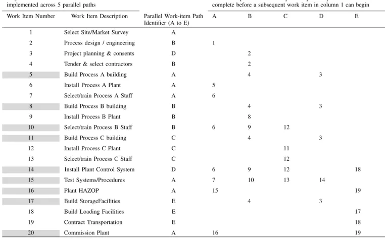
The work items of the example project are executed across five parallel pathways (see: P50 deterministic case precedence diagram Fig. 1) following a defined project network logic of work-item precedencies (Table 3).

Each of the parallel pathways, depending upon work-item duration assumptions, may represent the projects critical path. There is potential for the critical path to switch from one pathway of work items to another, depending on the duration values applied for each work item. The network logic for the example project identifies that nine of the twenty work items represent convergent points, with at least two other preceding work items leading into them (i.e., work items 5, 8, 10, 11, 14, 15, 16, 17 and 20). The relative performance of work items

(6)

Table 1.Example oil and gas field development facilities construction project with twenty individual work-item cost and duration input assumptions for three deterministic cases: fast, best estimate and slow cases for duration and low, best estimate and high cases for costs. Links between each time and cost case with depend upon the cost-time relationship used, e.g., for positive time-cost correlation slow time case could be linked with high cost cases, whereas

for negative time-cost correlation slow time case could be linked with high cost cases. Project Breakdown into 20 High-level Work

Items Implemented Across 5 Parallel Paths

Estimated Time to (Complete (Days)

Estimated Semi-fixed Cost to Complete Work Item ($ millions)

Estimated Variable Cost to Com-plete Work Item ($ millions / day) Work

Item Number

Work Item Description Fast

(P10) Best Estimate (P50) Slow (P90) Low (P10) Best Estimate (P50) High (P90) Low (P10) Best Estimate (P50) High (P90)

1 Select Site/Market Survey 50 75 100 20.0 30.0 40.0 0.300 0.500 0.750

2 Process design / engineering 60 80 100 20.0 30.0 40.0 1.250 1.500 1.750

3 Project planning & consents 60 90 120 20.0 30.0 40.0 0.300 0.500 0.800

4 Tender & select contractors 70 80 90 10.0 15.0 20.0 0.200 0.250 0.300

5 Build Process A building 120 150 180 30.0 50.0 70.0 2.500 3.000 3.500

6 Install Process A Plant 40 60 80 100.0 130.0 160.0 1.750 2.000 2.250

7 Select/train Process A Staff 30 40 50 5.0 10.0 15.0 0.750 1.000 1.250

8 Build Process B building 120 180 220 125.0 150.0 175.0 3.000 3.500 4.000

9 Install Process B Plant 50 75 100 120.0 150.0 180.0 2.000 2.500 3.000

10 Select/train Process B Staff 40 50 60 10.0 15.0 20.0 1.000 1.250 1.500

11 Build Process C building 100 125 150 25.0 40.0 55.0 2.250 2.500 2.750

12 Install Process C Plant 30 50 70 50.0 75.0 100.0 1.250 1.500 1.750

13 Select/train Process C Staff 20 30 40 5.0 10.0 15.0 0.500 0.750 1.000

14 Install Plant Control System 80 90 100 120.0 150.0 180.0 0.750 1.000 1.250

15 Test Systems/Procedures 20 30 40 15.0 20.0 25.0 0.750 1.000 1.250

16 Plant HAZOP 15 20 25 5.0 10.0 15.0 0.500 1.000 1.500

17 Build StorageFacilities 60 90 120 20.0 30.0 40.0 0.500 0.750 1.000

18 Build Loading Facilities 40 60 80 15.0 20.0 25.0 0.250 0.500 0.750

19 Contract Transportation 50 60 70 5.0 10.0 15.0 0.250 0.500 0.750

20 Commission Plant 30 40 50 15.0 20.0 25.0 1.500 2.000 2.500

Totals Duration totals ignore parallel paths: 1085 1475 1845 735.0 995.0 1255.0

Parallel Path Identifier 245 150 395 395 60 455 455 40 495 5 6 7 B 290 45 440 440 45 500 550 95 590 75 80 155 155 80 235 245 180 425 425 75 500 500 50 550 590 30 620 2 4 8 9 10 15 C 75 0 155 165 10 245 245 0 425 425 0 500 540 40 590 590 0 620 0 75 75 245 125 370 370 50 420 420 30 450 620 20 640 640 40 680 1 11 12 13 16 20 A 0 0 75 325 80 450 450 80 500 560 140 590 620 0 640 640 0 680 155 90 245 500 90 590 3 14 D 155 0 245 500 0 590

ESt D EF Critical path identified as thick red line 245 90 335 335 60 395 395 60 455

Work Item # ESt = Earliest start; D = Work item duration 17 18 19 E

EF = Earliest finish

LSt F LF LSt = Latest start; F = Float; LF = Latest finish 350 105 440 440 105 500 560 165 620

Critical Path Analysis for Project to Build a Example Plant Using a Precedence Network Diagram

Contract Transportation Select Site Market

survey Building Process C Process C Plant Train Process C Staff Planning / Consents Install Control System Work Item Description Build Storage Facilities Build Loading System

Plant HAZOP Commission Plant Building Process A Process A Plant Train Process A Staff Test Control System Process Engineering Tender/Select Contractors Building Process B Process B Plant Train Process B Staff

Fig. 1. High-level breakdown of twenty work items for the example oil and gas field development facilities construction project expressed as a precedence network with critical path items identified (i.e., thick arrows connecting work items with zero float) for the best estimate (P50) deterministic work-item assumptions (Table 1).

(7)

Table 2.Deterministic work-item time cost outcomes for five deterministic cases of the example project with positive linear or negative linear cost-time relationships.

Project Breakdown into 20 High-level Work Items Implemented Across 5 Parallel Paths

Assuming Positive Linear Correlation between Work Item Durations and Semi-fixed and Variable Cost Components

Assuming Negative Linear Correlation between Work Item Durations and Semi-fixed and Variable Cost Components

Total Work Item Costs ($ millions) at Specified Project Duration Percentiles

Work Item Number

Work Item Description Min

(P0) Fast (P10) Best Estimate (P50) Slow (P90) Max (P100) Min (P0) Low (P10) Best Estimate (P50) High (P90) Max (P100)

1 Select Site/Market Survey 15.6 35.0 67.5 115.0 161.0 76.0 77.5 67.5 50.0 27.0

2 Process design / engineering 57.8 95 150 215 274.9 133.6 145.0 150.0 145.0 133.6

3 Project planning & consents 16.0 38 75 136 194.6 84.4 88.0 75.0 56.0 28.2

4 Tender & select contractors 15.8 24 35 47 57.4 45.1 41.0 35.0 28.0 21.6

5 Build Process A building 214.4 330 500 700 883.8 460.0 490.0 500.0 480.0 441.9

6 Install Process A Plant 112.6 170 250 340 420.1 242.7 250.0 250.0 240.0 224.6

7 Select/train Process A Staff 13.0 28 50 78 103.4 50.9 52.5 50.0 42.5 32.8

8 Build Process B building 304.2 485 780 1055 1328.8 533.7 655.0 780.0 785.0 772.8

9 Install Process B Plant 143.2 220 338 480 613.6 305.6 330.0 337.5 320.0 287.5

10 Select/train Process B Staff 31.4 50 78 110 140.0 78.4 80.0 77.5 70.0 60.3

11 Build Process C building 176.2 250 353 468 569.7 302.7 330.0 352.5 362.5 361.4

12 Install Process C Plant 44.3 88 150 223 288.5 147.2 152.5 150.0 137.5 120.1

13 Select/train Process C Staff 4.5 15 33 55 76.9 33.4 35.0 32.5 25.0 15.3

14 Install Plant Control System 135.1 180 240 305 361.2 308.7 280.0 240.0 195.0 154.9

15 Test Systems/Procedures 17.5 30 50 75 98.9 46.3 50.0 50.0 45.0 37.3

16 Plant HAZOP 2.0 13 30 53 74.4 39.9 37.5 30.0 17.5 3.7

17 Build StorageFacilities 22.5 50 98 160 221.5 91.0 100.0 97.5 80.0 54.9

18 Build Loading Facilities 12.1 25 50 85 120.6 51.7 55.0 50.0 35.0 15.5

19 Contract Transportation 3.0 18 40 68 93.4 59.0 52.5 40.0 22.5 4.7

20 Commission Plant 35.0 60 100 150 197.8 92.7 100.0 100.0 90.0 74.6

Totals ($ millions) 1376 2202 3465 4916 6280 3183 3401.5 3465.0 3226.5 2872.7

leading into convergent points determines the critical path, and as performances vary during stochastic sampling and solution modifications, the exact route of the critical path can also vary.

The network calculation function forms an essential part of the STCTP memetic algorithm, because it performs forward and backward passes sequentially in the correct-work-item or-der across the network. For this study the STCTP memetic and all related analysis are coded in Visual Basic for Applications (VBA), with input and output located in a Microsoft Excel workbook. Applying the network logic defined in Table 3 to each set of work-item duration assumptions it provides key output metrics 1 (total project duration) and 2 (sum of all the work item durations ignoring parallel working). Key output metric 3 (total project costs) can also then be calculated, but will depend, independently of work-item precedencies, upon the duration-cost relationships applied to each work item es-tablishes values for five variables related to input assumptions for each work item (i.e., earliest start, earliest finish, latest start, float and latest finish; Fig. 1). The main challenges in solving practical project cost-time tradeoff problems with the memetic algorithm are the uncertainties in the input

cost-time assumptions for each work item and the relationships (e.g. correlations/dependencies) between the cost and time variables, which often differ from one work item to another.

5. Eight alternative work-item time-cost

rela-tionships ptimized

There is a myriad of possible time-cost relationships that could be applied to the work items of the example project. Also, different time-cost relationships could be applied to different work items and/or different relationships could be applied to time-semi-fixed cost and time-variable cost for each work item. To illustrate the impact of different work item time cost relationships, in the analysis present here, eight distinct work-item time-cost relationships are considered. To facilitate a comparison of the work-item time-cost relationship, for each case considered, one or other of the relationships is applied to all the work items, and to both cost distributions. Selecting the appropriate cost-time relationship for a specific project influences the efficiency and accuracy of the STCP solutions generated.

(8)

Table 3.PERT precedence network logic for the twenty work items of example project used to derive the full project duration (makespan) and cost for deterministic cases and all stochastic cases evaluated by the STCTP memetic algorithm.

Project work breakdown into 20 work items implemented across 5 parallel paths

Work item precedences of a specified parallel path that must be complete before a subsequent work item in column 1 can begin

Work Item Number Work Item Description Parallel Work-item Path

Identifier (A to E)

A B C D E

1 Select Site/Market Survey A

2 Process design / engineering B 1

3 Project planning & consents D 2

4 Tender & select contractors B 2

5 Build Process A building A 4 3

6 Install Process A Plant A 5

7 Select/train Process A Staff A 6

8 Build Process B building B 4 3

9 Install Process B Plant B 8

10 Select/train Process B Staff B 6 9 12

11 Build Process C building C 4 3

12 Install Process C Plant C 11

13 Select/train Process C Staff C 12

14 Install Plant Control System D 6 9 12 18

15 Test Systems/Procedures A 7 10 13 14

16 Plant HAZOP A 15 19

17 Build StorageFacilities E 4 3

18 Build Loading Facilities E 17

19 Contract Transportation E 18

20 Commission Plant A 16 19

Work items #5, 8, 10, 11, 14, 15, 16, 17 and 20 are convergent points in the network with two or more other work items feeding directly into them

Note to typesetters: please keep the grey background shading to highlighted cells in the first column of this table.

The eight relationships between work item time and cost are determined by formulas applied to the random number used to sample the work item duration probability distribu-tions, such that an appropriate fractional number (0, 1) can be derived for sampling the work item cost distributions. This can be achieved very easily in the stochastic sampling of the three distributions (duration, semi-fixed costs, variable cost) for each work item. The relationships evaluated are:

1. Negative Linear. If the random number (0, 1), Rd, is used to sample the duration probability distribution (expressed as a uniform distribution between P0 and P100 values Table 1), then the dependent fractional number Rc = 1−Rd is used

to sample the two cost distributions also expressed as uniform distributions.

2. Negative Sigmoidal. Same as relationship 1 except that the two cost distributions to sample are expressed as lognormal

distributions.

3. U-shaped. The relationship between Rd and Rc is

expressed by equation 1 with a uniform duration distribution and lognormal cost distributions being sampled.

Rc=    Rd≤a 1−Rd Rd> a min(0.999, (1−Rd) + (Rd−a)×b)) (1) where: a = change threshold, 0<a<1, a = 0.5 in the example presented; b = adjustment coefficient,b = 1.5 in the example presented;Rc is constrained by limits0< Rc <1.

4. Segmental. The relationship between Rd and Rc is

Rc=            Rd≤a min(c,1−(Rd×b)) Rd> a    Rd≤h max(g,(1−Rd)×f ×(1−Rd)) Rd< h (1−Rd)×e×(1−Rd))) (2)

(9)

where: a = change threshold, 0 < a < 1, a = 0.3 in the example presented; b = adjustment coefficient, b = 2.0 in the example presented; Rc is constrained by limits 0<Rc <1;

c = maximum limit, 0 < c < 1, c = 0.975 in the example presented; e = adjustment coefficient, e = 0.8 for RcS, e =

0.3 forRcV in example presented;f = adjustment coefficient, 0<f<1,f = 0.01 in example presented;g= maximum limit,

0 <g <1, g = 0.05 in example presented; h = adjustment coefficient, a<h<1, h= 0.75 in example presented; RcS

is the random number used to sample the semi-fixed cost distribution; RcV is the random number used to sample the

variable cost distribution.

5. V-shaped. The relationship between Rd and Rc is

Rc=    Rd≤a min(c,1−(Rd×b)) Rd> a min(c,(Rd−a)×e) (3)

where: a = change threshold, 0 < a < 1, a = 0.5 in the example presented; b = adjustment coefficient, b = 2.0 in the example presented; Rc is constrained by limits 0<Rc <1;

c = maximum limit, 0 < c < 1, c = 0.975 in the example presented, 0.0001 < 1 −(Rd×b) < c; e = adjustment

coefficient, e = 1.0 in the example presented for both RcS

andRcV.

6. Positive Linear. Same as relationship 1, except Rc =

Rd.

7. Positive Sigmoidal. Same as relationship 2, except

Rc=Rd.

8. Uncorrelated (independent). Time and cost distributions are all sampled as triangular distributions with independent random numbers. This case differs from the others in that a specific work item duration sampled in separate iterations could be associated with distinct costs, which is not the case for relationships 1 to 7. Hence, there is a greater range of uncertainty in the total project durations and costs generated with the uncorrelated relationship and no single reproducible optimum value.

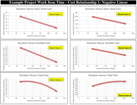
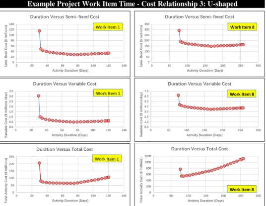
It is relatively easy using random number relationships that sample the work-item duration and cost probability distribu-tions to generate a wide range of continuous, stochastic, non-linear, cost relationships. Figs 2 to 5 illustrate the time-cost outcomes for relationships 1, 2, 3 and 8 for just work items #1 and #8 (Table 1), indicating the non-linear nature of the total work item time-cost outcomes. Work item #1 is selected because it is representative of the lower end of the range of cost and durations for all the work items. Work item #8 is selected because it is representative of the high end of the range of cost and durations for all the work items. Similar graphics for relationships 4, 5, 6 and 7 are included in the Appendix S.

Whereas the negative linear relationship (1) generates con-vex downwards total work item time-cost trends (Fig. 2), the positive linear relationship (6) generates convex upwards total work item time-cost trends. Whereas the negative sigmoidal relationship (2) generates convex downwards total work item time-cost trends (declining more rapidly towards the right, Fig.

3), the positive sigmoidal relationship (7) generates convex upwards total work item time-cost trends (rising more rapidly towards the right). The segmental relationship (4) generates convex downwards total work item time-cost trends with three distinct segments resulting in the central segment being significantly lower in cost than the left end of the trend and slightly lower than the right end of the trend. The V-shaped relationship (4) generates two convex downwards total work item time-cost trends that intersect at distinct minima in the central area of the duration range for each work item with three distinct segments resulting in the central segment being significantly lower in cost than the left end of the trend and slightly lower than the right end of the trend.

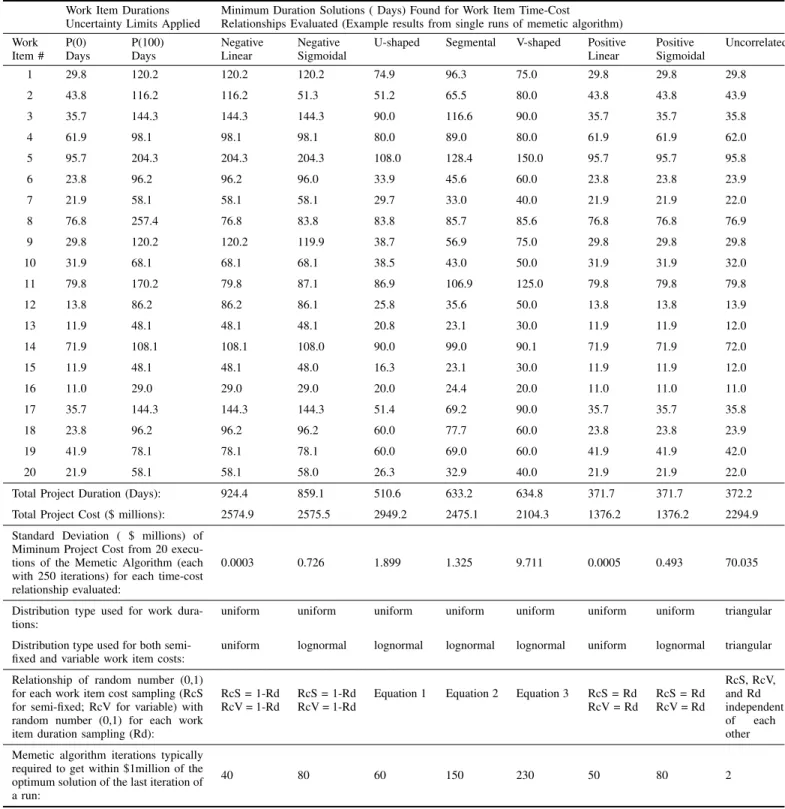
The STCTP to locate the lowest total project cost was eval-uated with the memetic algorithm for each of the eight time-cost relationships described applied to the example project. The algorithm was executed using the following control values: M = 250, N = 200, Q = 50. Twenty distinct executions of the algorithm were performed for each time-cost relationship and the results analyzed statistically to provide means and standard deviations of the optima found. The minimum total project cost solutions (i.e., the optimum work item durations, total project duration and total project cost) for each time-cost relationship case are listed in Table 4.

Standard deviations of the optimum total-project-cost so-lutions found for twenty executions of the memetic algorithm are very low for work-item time-cost relationships 1, 2, 3, 4, 6 and 7 (Table 4), suggesting that the algorithm is consistent in its performance. For these six relationships, the algorithm is finding solutions within $1 million of the optimum value after 40 to 100 iterations (i.e., well within the 250 iterations performed in each execution). For work-item time-cost rela-tionship 5 the algorithm typically takes 230 or so iterations to find solutions within $1 million of the optimum, resulting in a slightly higher standard deviation of $9.7 million (Table 4). Performing more iterations for relationship 5 reduces the standard deviation of the optimum values found in multiple run.

For work-item time-cost relationship 8 the standard de-viation of the optimum total-project-cost solutions found is much higher ($70 million), because of the stochastic nature of that relationship (Fig. 5). There is a very low chance of stochastically sampling close to the P0 values of each work item duration and cost distribution with three independently selected random numbers. Hence, the optimum values found in each run of the memetic algorithm are not near the global optimum that could possibly exist, which would be very close to the P0 values of all distributions (i.e., $1376 million total project costs). Therefore, if there is no defined relationship between work item durations and costs the memetic algorithm is not likely to find possible global optimums that exist with very low probabilities of occurrence. Nevertheless, some useful information can be derived from such runs in terms of the Pareto frontiers they reveal. The optimum solution for relationship 8 is typically found in iteration #2. This is because the random solutions of iteration 1 (Mh1) are ranked and the high-ranking population Q consists of the work-item durations that are associated with lowest total project

(10)

Example Project Work Item Time - Cost Relationship 1: Negative Linear 0 10 20 30 40 50 60 0 20 40 60 80 100 120 140 Sem i-fix ed C o st ( $ m il li o ns)

Activity Duration (Days)

Duration Versus Semi-fixed Cost

Work Item 1 0.0 0.1 0.2 0.3 0.4 0.5 0.6 0.7 0.8 0.9 1.0 0 20 40 60 80 100 120 140 Var iabl e C o st ($ m il li o ns /day )

Duration Versus Variable Cost

Work Item 1 0 10 20 30 40 50 60 70 80 90 0 20 40 60 80 100 120 140 T o tal A ct iv it y C o st ( $ m il li o ns)

Duration Versus Total Cost

Work Item 1 0 100 200 300 400 500 600 700 800 900 0 50 100 150 200 250 300 T o tal Ac ti vi ty C o st ( $ m il li o n s)

Work Item 8 0 50 100 150 200 250 0 50 100 150 200 250 300 S emi -fi xed C os t ($ milli on s)

Work Item 8 0.0 0.5 1.0 1.5 2.0 2.5 3.0 3.5 4.0 4.5 5.0 0 50 100 150 200 250 300 Va ri abl e C o st ( $ m il li o n s/day)

Work Item 8

Fig. 2. Time-cost trends for work items 1 and 8 of example project for time-cost relationship 1. Negative Linear.

Example Project Work Item Time - Cost Relationship 2: Negative Sigmoidal

0 50 100 150 200 250 0 20 40 60 80 100 120 140 To ta l A ct ivi ty C o st ( $ m il li o ns)

Work Item 1 0 100 200 300 400 500 600 700 800 900 0 50 100 150 200 250 300 T o tal Ac ti vi ty C o st ( $ m il li o n s)

Work Item 8 0 20 40 60 80 100 120 140 0 20 40 60 80 100 120 140 Sem i-fix ed C o st ($ m il li o ns)

Work Item 1 0 50 100 150 200 250 300 350 0 50 100 150 200 250 300 S emi -fi xed C os t ( $ mil lio n s)

Work Item 8 0.0 0.5 1.0 1.5 2.0 2.5 3.0 3.5 0 20 40 60 80 100 120 140 V ar iab le C o st ( $ m il li o ns /d ay)

Work Item 1 0.0 1.0 2.0 3.0 4.0 5.0 6.0 7.0 0 50 100 150 200 250 300 V ar ia bl e C o st ( $ m il li o n s/day)

Work Item 8

(11)

Example Project Work Item Time - Cost Relationship 3: U-shaped 0 50 100 150 200 250 0 20 40 60 80 100 120 140 To tal A ctivity C o st ($ m il li o ns)

Work Item 1 0 200 400 600 800 1000 1200 0 50 100 150 200 250 300 To ta l A ct ivi ty C o st ( $ m il li o ns)

Work Item 8 0 20 40 60 80 100 120 140 0 20 40 60 80 100 120 140 Sem i-fix ed C o st ($ m il li o ns)

Work Item 1 0.0 0.5 1.0 1.5 2.0 2.5 3.0 3.5 0 20 40 60 80 100 120 140 V ar iab le C o st ( $ m il li o ns /d ay)

Work Item 1 0.0 1.0 2.0 3.0 4.0 5.0 6.0 7.0 0 50 100 150 200 250 300 Var iab le C o st ( $ m il li o ns/d ay)

Work Item 8 0 50 100 150 200 250 300 350 0 50 100 150 200 250 300 Sem i-fix ed C o st ($ m il li o ns)

Work Item 8

Fig. 4. Time-cost trends for work items 1 and 8 of example project for time-cost relationship 3. U-shaped.

Example Project Work Item Time - Cost Relationship 8: Uncorrelated

0 10 20 30 40 50 60 0 20 40 60 80 100 120 140 Sem i-fix ed C o st ($ m il li o ns)

Duration Versus Semi-fixed CostWork Item 1

100 110 120 130 140 150 160 170 180 190 200 0 50 100 150 200 250 300 S em i-fi xed C os t ( $ mil lio n s)

Duration Versus Semi-fixed CostWork Item 8

0.0 0.1 0.2 0.3 0.4 0.5 0.6 0.7 0.8 0.9 1.0 0 20 40 60 80 100 120 140 V ar ia bl e C o st ( $ m il li o n s/day)

Duration Versus Variable Cost Work Item 1

2.0 2.5 3.0 3.5 4.0 4.5 0 50 100 150 200 250 300 Va ri abl e C o st ( $ m il li o n s/day)

Duration Versus Variable Cost Work Item 8

0 20 40 60 80 100 120 140 0 20 40 60 80 100 120 140 To ta l A ct ivi ty C o st ( $ m il li o ns)

Duration Versus Total Cost Work Item 1

0 200 400 600 800 1000 1200 0 50 100 150 200 250 300 Tota l Ac tiv ity C os t ( $ mil lio n s)

Duration Versus Total Cost Work Item 8

(12)

Table 4.Example project’s optimum solutions found by STCTP memetic algorithm for work item durations, total project durations and total project costs applying eight distinct work-item time-cost relationships applied.

Work Item Durations Uncertainty Limits Applied

Minimum Duration Solutions ( Days) Found for Work Item Time-Cost

Relationships Evaluated (Example results from single runs of memetic algorithm) Work Item # P(0) Days P(100) Days Negative Linear Negative Sigmoidal

U-shaped Segmental V-shaped Positive

Linear Positive Sigmoidal Uncorrelated 1 29.8 120.2 120.2 120.2 74.9 96.3 75.0 29.8 29.8 29.8 2 43.8 116.2 116.2 51.3 51.2 65.5 80.0 43.8 43.8 43.9 3 35.7 144.3 144.3 144.3 90.0 116.6 90.0 35.7 35.7 35.8 4 61.9 98.1 98.1 98.1 80.0 89.0 80.0 61.9 61.9 62.0 5 95.7 204.3 204.3 204.3 108.0 128.4 150.0 95.7 95.7 95.8 6 23.8 96.2 96.2 96.0 33.9 45.6 60.0 23.8 23.8 23.9 7 21.9 58.1 58.1 58.1 29.7 33.0 40.0 21.9 21.9 22.0 8 76.8 257.4 76.8 83.8 83.8 85.7 85.6 76.8 76.8 76.9 9 29.8 120.2 120.2 119.9 38.7 56.9 75.0 29.8 29.8 29.8 10 31.9 68.1 68.1 68.1 38.5 43.0 50.0 31.9 31.9 32.0 11 79.8 170.2 79.8 87.1 86.9 106.9 125.0 79.8 79.8 79.8 12 13.8 86.2 86.2 86.1 25.8 35.6 50.0 13.8 13.8 13.9 13 11.9 48.1 48.1 48.1 20.8 23.1 30.0 11.9 11.9 12.0 14 71.9 108.1 108.1 108.0 90.0 99.0 90.1 71.9 71.9 72.0 15 11.9 48.1 48.1 48.0 16.3 23.1 30.0 11.9 11.9 12.0 16 11.0 29.0 29.0 29.0 20.0 24.4 20.0 11.0 11.0 11.0 17 35.7 144.3 144.3 144.3 51.4 69.2 90.0 35.7 35.7 35.8 18 23.8 96.2 96.2 96.2 60.0 77.7 60.0 23.8 23.8 23.9 19 41.9 78.1 78.1 78.1 60.0 69.0 60.0 41.9 41.9 42.0 20 21.9 58.1 58.1 58.0 26.3 32.9 40.0 21.9 21.9 22.0

Total Project Duration (Days): 924.4 859.1 510.6 633.2 634.8 371.7 371.7 372.2

Total Project Cost ($ millions): 2574.9 2575.5 2949.2 2475.1 2104.3 1376.2 1376.2 2294.9

Standard Deviation ( $ millions) of Miminum Project Cost from 20 execu-tions of the Memetic Algorithm (each with 250 iterations) for each time-cost relationship evaluated:

0.0003 0.726 1.899 1.325 9.711 0.0005 0.493 70.035

Distribution type used for work dura-tions:

uniform uniform uniform uniform uniform uniform uniform triangular

Distribution type used for both semi-fixed and variable work item costs:

uniform lognormal lognormal lognormal lognormal uniform lognormal triangular

Relationship of random number (0,1) for each work item cost sampling (RcS for semi-fixed; RcV for variable) with random number (0,1) for each work item duration sampling (Rd):

RcS = 1-Rd RcV = 1-Rd

Equation 1 Equation 2 Equation 3 RcS = Rd

RcV = Rd RcS = Rd RcV = Rd RcS, RcV, and Rd independent of each other Memetic algorithm iterations typically

required to get within $1million of the optimum solution of the last iteration of a run:

40 80 60 150 230 50 80 2

Note: equations 1, 2 and 3, depending on the coefficient values input, may sample just portions of the full cost distributions, not the full range between P0 and P100.

(13)

costs in that population. Metaheuristics Mh2 to Mh8 produce modifications of those Qsolutions from iteration 2 onwards, but the independent nature of work-item duration and costs, means that many of the modifications will lead to-higher-project-cost outcomes. Hence, the quality of sub-population

Q in terms of total project cost for this relationship is less likely to improve as iterations progress, as it does for the other defined work-item duration to cost relationships.

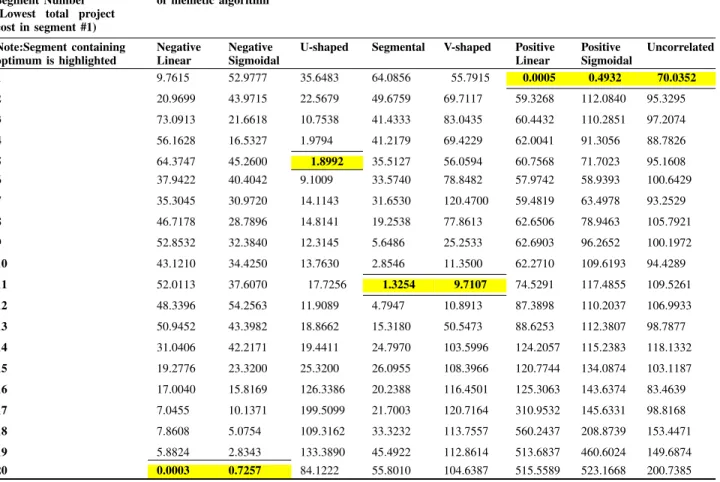
Table 5 lists key statistics for the optimum results of total example project costs along the Pareto frontier with the eight-distinct work-item time-cost relationships applied. The lower portion of Table 5 reveals the minimum values associated with each of the twenty project duration intervals evaluated to form the Pareto frontier, highlighting the overall optimum value found. As expected, work-item time-cost relationships 3, 4 and 5 have their overall optimum values some distance from the ends of their Pareto frontiers, whereas for the other relationships the optimum values found are located at one end of their Pareto frontier.

The upper portion of Table 5 reveals that the further from the overall minimum value found a segment is located on the Pareto frontier the higher the standard deviation associated with the optimum value is likely to be for multiple executions of the algorithm. The explanation for this is that the memetic-optimization algorithm is focused on locating the overall optimum and will progressively locate more and more of its trial solutions in the vicinity of that optimum, but fewer and fewer trial solutions will test durations further from the overall optimum. Hence, in the duration intervals along the Pareto frontier where more trials have searched the standard deviations of the minimum values found is likely to be lower. The drop in standard deviations at the opposite end of the Pareto frontier to the overall optimum in the cases of work-item cost-time relationships 1 and 2 reflects very low numbers of trials actually testing those distal duration intervals.

In order to evaluate certain intervals of the Pareto frontier in more detail, to obtain more accurate local optima within them, it is necessary to rerun the algorithm placing upper and lower constraints on total project costs at the boundaries of the intervals of interests (i.e., narrowing the feasible solution space to be searched). This would force the algorithm to locate all of its trials within those boundaries and thereby reduce the standard deviation on the local minimum values found.

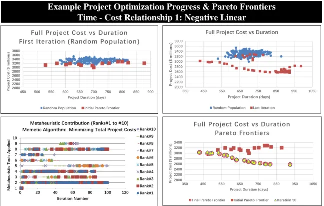
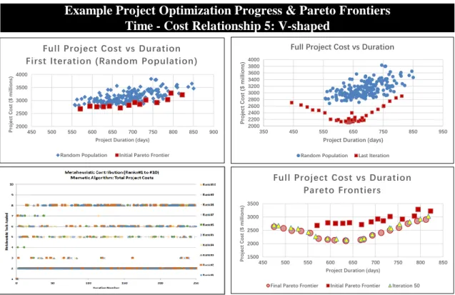
Figs 6 to 9 each provide four images that illustrate the progress the memetic algorithm makes in locating the overall optimum and the Pareto frontier found for different work-item cost-time relationships. The upper-left image illustrates the results of the random population generated by the first iteration of the algorithm in terms of total project duration and costs of each solution with the Pareto frontier highlighted. The upper-right image shows the solutions produced by the last iteration of the algorithm compared with the random population of the first iteration. Note that many of the solutions in the last iteration are located close to the overall optimum with others scattered along the Pareto frontier (due to the functioning of Mh3). The lower-right image shows how the optimum values along the Pareto frontier have evolved comparing the results of iterations 1, 50 and 250. The lower-left image

provides a metaheuristic profile, which is analyzed below. Fig. 6 (Negative-linear relationship) reveals that by iteration 50 the end of the Pareto frontier closest to the overall optimum is well established after 50 iterations, with minor improvements made (by Mh3 mainly) to the distal portion of the Pareto frontier in later iterations.

Figs 7 and 8 (segmental and V-shaped relationships re-spectively) also show that the algorithm has located the vicinity of the overall optimum by iteration 50 and achieves minor improvements mainly in the segments of the Pareto frontier distal from the overall optimum in later iterations. Fig. 9 (Uncorrelated/independent relationship) reveals that the solutions of the final iteration are more widely spread than for the other relationships, but are concentrated in distinctly lower project duration and cost regions than the solutions of the first iteration. This suggest that even with no correlations between work-item duration and cost the memetic algorithm can identify meaningful portions of a Pareto frontier. Very few improvements are made to the distal end of the Pareto frontier from iteration 1 to 250 in this case, indicating that very few solutions search this area, which is also supported by the high standard deviations (Table 5).

6. Performance profiles of metaheuristics in the

optimization process

The metaheuristic profile (MHP), a recently proposed technique (Wood, 2016a,b), depicted in the lower-left image of Figs 6 to 9 provides a useful performance record of the various metaheuristics involved in the memetic algorithm in generating top-ten ranking solutions in each iteration performed. Meta-heuristics Mh2, Mh4 and Mh8 provide most top-ten solutions for the negative-linear relationship (Fig. 6), with the Mh3 and Mh5 making significant supporting contributions. The negative-sigmoidal relationship (not shown) displays a similar metaheuristic profile. Note Mh10, by nature of its defined function, is not going to make any top-ten contributions for any of the time-cost relationships, but is nonetheless likely to aid exploration of the wide feasible solution space. This profile is expressed for just the first 100 iterations as the optimum value is well established by that point.

Metaheuristics Mh2, Mh6 and Mh8 provide most top-ten solutions for the segmental relationship (Fig. 7), with Mh3 and Mh5 making supporting contributions. This profile is expressed for all 250 iterations as the optimum value is found in later iterations. The U-shaped relationship (not shown) displays a similar metaheuristic profile. Metaheuristics Mh2, Mh6 and Mh8 provide most top-ten solutions for the V-shaped relationship (Fig. 8), with Mh5 making a significant supporting contribution, but Mh3 much less so. Note Mh4 makes almost no contribution to the top-ten solutions in these two cases. Metaheuristics Mh2, Mh3, Mh4, Mh6 and Mh7 provide most top-ten solutions for the uncorrelated relationship (Fig. 9), with Mh8 making a minor supporting contribution. It is Mh3, in this case, that finds the rank #1 solution in iteration 2 that is not improved upon subsequently. Mh2 and Mh4 make the dominant contributions for the positive linear and positive sigmoidal cases (not shown). Metaheuristic profiles for the

(14)

Table 5.Example project’s key statistics of optimum results for total project costs along the Pareto frontier with eight distinct work-item time-cost relationships applied.

Pareto Frontier Segment Number (Lowest total project cost in segment #1)

Standard deviations of optimal project costs ($millions) for each pareto frontier segment over 20 runs of memetic algorithm Note:Segment containing optimum is highlighted Negative Linear Negative Sigmoidal

U-shaped Segmental V-shaped Positive

Linear Positive Sigmoidal Uncorrelated 1 9.7615 52.9777 35.6483 64.0856 55.7915 0.0005 0.4932 70.0352 2 20.9699 43.9715 22.5679 49.6759 69.7117 59.3268 112.0840 95.3295 3 73.0913 21.6618 10.7538 41.4333 83.0435 60.4432 110.2851 97.2074 4 56.1628 16.5327 1.9794 41.2179 69.4229 62.0041 91.3056 88.7826 5 64.3747 45.2600 1.8992 35.5127 56.0594 60.7568 71.7023 95.1608 6 37.9422 40.4042 9.1009 33.5740 78.8482 57.9742 58.9393 100.6429 7 35.3045 30.9720 14.1143 31.6530 120.4700 59.4819 63.4978 93.2529 8 46.7178 28.7896 14.8141 19.2538 77.8613 62.6506 78.9463 105.7921 9 52.8532 32.3840 12.3145 5.6486 25.2533 62.6903 96.2652 100.1972 10 43.1210 34.4250 13.7630 2.8546 11.3500 62.2710 109.6193 94.4289 11 52.0113 37.6070 17.7256 1.3254 9.7107 74.5291 117.4855 109.5261 12 48.3396 54.2563 11.9089 4.7947 10.8913 87.3898 110.2037 106.9933 13 50.9452 43.3982 18.8662 15.3180 50.5473 88.6253 112.3807 98.7877 14 31.0406 42.2171 19.4411 24.7970 103.5996 124.2057 115.2383 118.1332 15 19.2776 23.3200 25.3200 26.0955 108.3966 120.7744 134.0874 103.1187 16 17.0040 15.8169 126.3386 20.2388 116.4501 125.3063 143.6374 83.4639 17 7.0455 10.1371 199.5099 21.7003 120.7164 310.9532 145.6331 98.8168 18 7.8608 5.0754 109.3162 33.3232 113.7557 560.2437 208.8739 153.4471 19 5.8824 2.8343 133.3890 45.4922 112.8614 513.6837 460.6024 149.6874 20 0.0003 0.7257 84.1222 55.8010 104.6387 515.5589 523.1668 200.7385 Pareto Frontier Segment Number (Lowest total project cost in segment #1)

Minimum project costs ($millions) found within each pareto frontier segment over 20 runs of memetic algorithm 1 3008 2900 2957 2681 2706 1376 1376 2110 2 2981 2872 2951 2672 2518 1689 1608 2181 3 2983 2861 2949 2600 2509 1727 1666 2204 4 2901 2856 2949 2556 2486 1793 1794 2266 5 2870 2829 2949 2545 2432 1835 1869 2300 6 2847 2793 2949 2516 2285 1889 1971 2331 7 2819 2790 2950 2484 2176 1937 2005 2368 8 2762 2786 2967 2479 2129 1978 2034 2426 9 2758 2745 2986 2477 2116 2045 2063 2486 10 2699 2746 3005 2475 2104 2113 2105 2528 11 2661 2716 3028 2475 2104 2154 2141 2608 12 2659 2628 3055 2475 2104 2259 2175 2620 13 2650 2618 3080 2476 2123 2350 2282 2682 14 2629 2603 3106 2478 2124 2397 2319 2710 15 2607 2586 3120 2492 2173 2520 2352 2833 16 2600 2583 3146 2535 2264 2559 2379 2908 17 2593 2575 3210 2562 2328 2657 2509 2936 18 2584 2575 3524 2585 2535 2719 2565 3089 19 2575 2574 3518 2602 2645 2876 2893 3146 20 2575 2574 3669 2612 2819 2965 2981 3193