Logistics Capacity Planning: A
Stochastic Bin Packing
Formulation and a Progressive
Hedging Meta-Heuristic
Teodor Gabriel Crainic Luca Gobbato
Guido Perboli Walter Rei
December 2014
1 Interuniversity Research Centre on Enterprise Networks, Logistics and Transportation (CIRRELT) 2 Department of Management and Technology, Université du Québec à Montréal, P.O. Box 8888,
Station Centre-Ville, Montréal, Canada H3C 3P8
3 Department of Control and Computer Engineering, Politecnicò di Torino, Corso Duca degli
Abruzzi, 24 - I-10129 Torino, Italy
Abstract. In this paper, we consider the logistics capacity planning problem arising in the context of supply-chain management. We address, in particular, the tactical-planning problem of determining the quantity of capacity units, hereafter called bins, of different types to secure for the next period of activity, given the uncertainty on future needs in terms of demand for loads (items) to be moved or stored, and the availability and costs of capacity for these movements or storage activities. We propose a modeling framework for this problem introducing a new class of bin packing problems, the Stochastic Variable Cost and Size Bin Packing Problem (SVCSBPP). The resulting two-stage stochastic formulation with recourse assigns to the first stage the tactical capacity-planning decisions of selecting bins, while the second stage models the subsequent adjustments to the plan, securing extra bins, when needed, and packing the items into the selected bins each time the plan is applied and new information becomes known. We propose a new meta-heuristic to address this formulation. The meta-meta-heuristic is based on progressive hedging ideas and includes several advanced strategies to accelerate the search and efficiently address the symmetry strongly present in the problem considered due to the presence of several equivalent bins of each type. Extensive computational results for a large set of instances support the claim of validity for the model, efficiency for the solution method proposed, and quality and robustness for the solutions obtained. The method is also used to explore the impact on the capacity plan and the recourse to spot-market capacity of a quite wide range of variations in the uncertain parameters and the economic environment of the firm.
Keywords: Logistics capacity planning, uncertainty, stochastic variable cost and size bin packing, stochastic programming, progressive hedging.
Acknowledgements.Partial funding for this project was provided by the Italian University and Research Ministry under the UrbeLOG project-Smart Cities and Communities. Partial funding was also provided by the Natural Sciences and Engineering Research Council of Canada (NSERC), through its Discovery Grant program. We gratefully acknowledge the support of Fonds de recherche du Québec – Nature et technologies (FRQNT) through their infrastructure grants.
Results and views expressed in this publication are the sole responsibility of the authors and do not necessarily reflect those of CIRRELT.
Les résultats et opinions contenus dans cette publication ne reflètent pas nécessairement la position du CIRRELT et n'engagent pas sa responsabilité.
_____________________________
* Corresponding author: [email protected] Dépôt légal – Bibliothèque et Archives nationales du Québec
1
Introduction
The efficient consolidation of goods for movement and storage is essential for companies that aim to be competitive in the market and fulfill customer demand in a cost-efficient and flexible manner (Crainic et al., 2013b). Modern companies manufacture or acquire goods that are then consolidated into appropriate containers, which are in turn consol-idated for long-distance, often international, transportation into ships or trains. Before reaching the final customer, the goods are stored for varying periods into a number of depots, warehouses or distribution centers. All these activities require that capacity, as containers, ship or train slots, motor carrier tractors, and warehousing space, be available when and where needed.
The planning of such logistics capacity directly affects the distribution and operating costs of the company, and therefore is a major challenge in supply chain management (Monczka et al., 2008). Logistics capacity planning as a tactical planning decision ad-dresses the needs of the company for sufficient capacity to move and store its goods to meet demand in the next cycle of its activities. When tactical decisions are made, the company does not have detailed knowledge of many decision parameters such as the fu-ture demand and, thus, its real needs in terms of loads to be moved or stored, and the availability and costs of capacity. Such information becomes available, however, at the time for operational decisions, and it can be used to reconsider and update the capacity planning.
Our goal is providing models and methods to support decision making in logistics capacity planning. We focus, in particular, on the relation between a firm and its lo-gistics capacity provider, and the tactical-planning problem of determining the quantity of capacity to secure for the next period of activity (from four to twelve months) given the uncertainty on future needs and availabilities. We propose a two-stage stochastic programming formulation based on the Variable Cost and Size Bin Packing Problem
(VCSBPP) (Crainic et al., 2011b) to address this issue, together with an efficient meta-heuristic based on Progressive Hedging principles (Rockafellar and Wets, 1991).
Bin packing models offer important decision tools for transportation and logistics (Perboli et al., 2014a). In bin packing problems, various items must be packed into containers or other types of boxes and spaces, generally called bins, the particular char-acteristics of items and bins in terms of capacities and costs generating a rich set of problem settings and formulation. The packing formulations currently proposed in the literature deal only partially, however, with the requirements of capacity planning, as most research has explored operational issues only. Thus, most of the literature address-ing bin packaddress-ing and uncertainty, focuses on modeladdress-ing uncertainty in item arrival, leadaddress-ing to the so-called on-line packing problem (Seiden, 2002). Studies focusing on stochastic versions of bin packing problems for strategic and tactical planning applications are few and recent. Perboli et al. (2012, 2014b) introduced stochastic costs and profits into a bin
packing and a knapsack problems. Crainic et al. (2014a) proposed a stochastic extension of the VCSBPP (Crainic et al., 2011b) for the capacity planning problem with demand uncertainty in terms of the number of items and their volumes.
These problems were formulated as two-stage integer stochastic programs with re-course (Birge and Louveaux, 1997). This approach separates the a priori planning de-cisions, taken under uncertainty before the activity cycle starts, and the adjustments performed at each period of operations once information becomes available. The former makes up the first stage of the model, while the recourse actions, defining the admissible adjustments to the plan, make up the second stage. Discretization methods are usu-ally applied to approximate the probability distribution of the random parameters using a finite-dimension scenario tree (Mayer, 1998). Using the scenario tree approximation, one can reduce two-stage integer stochastic programs to deterministic linear programs with integer decision variables of generally very large dimensions, beyond the reach of exact methods. Indeed, Crainic et al. (2011a) and Crainic et al. (2014b) shown that a state-of-the-art MIP solver struggles to solve even small instances of stochastic VCS-BPP formulations. Our goal is to successfully solve much larger problems. Therefore, heuristics are required.
Most solution approaches in the literature rely on decomposition techniques (Rosa and Ruszczynski, 1996; Higle and Sen, 1996). TheProgressive Hedging (PH) algorithm, initially proposed by Rockafellar and Wets (1991) for stochastic convex programs, has emerged as an effective meta-heuristic for addressing stochastic programs with discrete decision variables (e.g., Crainic et al., 2011a; Carpentier et al., 2013; Crainic et al., 2014b; Veliz et al., 2014). It mitigates the computational difficulty associated with large problem instances by using augmented Lagrangian relaxation to decompose the stochastic program by scenario. It then iteratively solves penalized versions of the subproblems, gradually enforcing the consensus relative to the first-stage decision variables. PH enables the use of specialized heuristic methods for the subproblems, fast and accurate methods being crucial to the overall efficiency of the method, because subproblems are repeatedly solved.
The contribution of this paper is threefold.
1. A modeling framework for securing logistics capacity for a tactical-planning horizon, while explicitly considering uncertainty in both supply, availability and cost of various bin types, and demand as the number and dimension of items. In doing so, we introduce a new class of stochastic bin packing problems, namely theStochastic Variable Cost and Size Bin Packing Problem (SVCSBPP).
2. A new and effective meta-heuristic for the two-stage formulation of the SVCS-BPP. The proposed solution method is based on PH ideas, uses the heuristic of Crainic et al. (2011b) to address the scenario subproblems, and includes several enhancements to deal with the particular characteristics of the problem. One
par-ticularly challenging characteristic is the symmetry inherent to packing problems, and strongly present in the SVCSBPP due to the presence of several equivalent bins of each type. The many equivalent but apparently different solutions in their choice of bins may significantly impair the efficiency of a PH-based meta-heuristic. Several strategies are thus proposed, including the definition of a new temporary global solution, heuristic penalty adjustments, and bundle fixing to reduce the bin selection at each iteration.
3. An extensive computational campaign using a large set of instances of various di-mensions and combinations of different levels of variability in the stochastic param-eters. The campaign includes the assessment of the efficiency of the meta-heuristic, the evaluation of the interest to explicitly consider uncertainty, an analysis of the impact of problem characteristics on capacity planning, the structure of solutions and the sensitivity to changes in data in particular, as well as an evaluation of the robustness of the decisions over a long time period under different economic and demand-evolution scenarios.
The numerical analysis indicates that the value of uncertainty is significant and that the proposed PH meta-heuristic finds good solutions fast. They also show that the proposed formulation is able to represent the impact of various levels of variation in the random parameters, and yields good-quality plans (solutions). Indeed, solutions are conservative and minimize the need to adjust the plan. Moreover, the capacity plan is robust (variations in the demand implying low operating costs) and relatively insensitive to changes. One may therefore conclude that SVCSBPP is a useful tool for logistics capacity planning under uncertainty, and that the proposed meta-heuristic is an appropriate and efficient solver for this class of formulations.
The paper is organized as follows. Section 2 details the logistics capacity planning problem we address in this paper. Section 3 presents the formulation of the problem. A lower bound and the meta-heuristic solution method are introduced in Sections 4 and 5, respectively. Section 6 presents the experimental plan and analyzes the computational results. Section 7 provides concluding remarks.
2
Logistics Capacity Planning
The tactical capacity planning problem we address is relevant in many contexts, e.g., manufacturing firms desiring to secure transportation capacity to bring in their resources or to distribute their products, wholesalers and retailers planning for transportation and storage capacity to support their procurement and sales processes, and logistics service providers securing capacity contracts with carriers for long-distance, regular shipments. Manufacturing and whole/retail distribution firms may negotiate directly with carriers
and owners/managers of storage space but, very often, they do business with a logistic service provider. Consequently, in order to simplify the presentation, but without loss of generality, we describe the problem within the context of the process of contract procurement between a major retail firm and a third-party logistics (capacity) service provider (3PL).
In the contemporary economic and business environment, firms are engaged in a con-tinuous procurement process (Aissaoui et al., 2007; Rizk et al., 2008), and engage in various collaborations with its supply-chain partners. Such inter-firm alliances yield sev-eral benefits, including a reduction in inefficiencies, total cost, and financial risks. The greatest advantages result from the outsourcing of logistics activities to a 3PL (Marasco, 2008). The overall supply-chain process may then be summarized as follows. The firm regularly orders products from suppliers in a given geographical region, according to current inventories, short-term forecast demand, estimated lead times, and specific pro-curement and inventory policies (Bertazzi and Speranza, 2005; Bertazzi et al., 2007) The suppliers are instructed to deliver their goods to a consolidation center (Crainic and Kim, 2007; Bertazzi and Speranza, 2012). The 3PL then consolidates the goods into containers and ensures their shipping, by consolidating these containers with those of other customers into the slots it secured on long-haul cariers, e.g., ships and trains (Chen et al., 2001; Crainic et al., 2013a), which generally operate according to a fixed schedule, e.g., twice a week.
A key factor in this process is the procurement of sufficient capacity, that we express in the following in terms of bins, at different locations in the network and for varying periods of time, to satisfy the demand. This entails negotiations with the 3PL to book the necessary capacitya priori, before operations start, at the best rate (Ford, 2001). The results of these negotiations often take the form of medium-term contracts specifying both the capacity to be used, thequantity and the type of bins, and the additional services to be performed (storage, transportation, bin operations, etc.) for a given planning horizon, e.g., a semester or a year. These contracts guarantee a regular volume of business to the 3PL (e.g., a fixed number of containers to ship every week for the next semester), which ensures a cost-effective service to the firm.
We refer to the costs of bins selected in advance asfixed costs because they are fixed by the contract and thus represent the specific rates offered by the 3PL for bins of different sizes. The values of the fixed costs are in practice influenced by several factors, including bin size, bin type (e.g., thermal or refrigerated containers), physical handling operations required, the time period for which the bin is to be used, and the economic characteristics of the departure location (e.g., access rules and costs). The result of negotiations and the scope of the capacity planning problem then is a tactical plan defining these quantities for the firm at each location, given the proposed bin types and costs and an estimation of the demand over the planning horizon. The plan thus specifies the set of bins of particular volumes and fixed costs to be made available at each location to ship the estimated items.
Given the time lag that usually exists between the signing of the contracts and the logistics operations, the negotiations are performed under uncertainty, without all the necessary information concerning thedemand, expressed as a number of items of variable sizes to be shipped or stored at the particular locations. At each application of the plan, variations in the demand may thus yield numbers and sizes of items that differ from the estimation used at negotiation. These variations then require further negotiations with the 3PL and an adjustment of the plan when the booked capacity is not sufficient. Extra capacity (additional bins available at the shipping date) must then be purchased, generally at a much higher cost (the so-called spot -market value) than the fare negotiated initially. Moreover, while the 3PL generally ensures the planned capacity for the firm, the extra capacity may not be available when needed. The extra capacity must therefore be considered stochastic as well.
The Stochastic Variable Cost and Size Bin Packing Problem thus consists in deter-mining the most cost-effective tactical plan, including the costs of the bins secured within the negotiations and the possible cost of updating the plan and securing extra capacity when the actual demand and the spot-market bin availability become known.
We propose a two-stage stochastic programming formulation, where the first stage concerns the selection of bins, and the second stage concerns the acquisition of extra capacity when the actual demand information is revealed. The next section details the Stochastic Variable Cost and Size Bin Packing (VCSBP) formulation.
3
The VCSBPModel
Let T be the finite set of bin types, each type being defined by the volume and fixed cost associated with its bins. Let Vτ and fτ respectively be the volume and fixed cost
associated with bins of type τ ∈ T. We define Jτ to be the set of available bins of type τ and J =∪τJτ to be the set of available bins at the first stage.
Let set Ω be the sample space of the random event, whereω ∈Ω defines a particular realization. Let vector ξ contain the stochastic parameters defined in the model, and
ξ(ω) be a given realization of this random vector. Let the first-stage variables be yjτ = 1 if bin j ∈ Jτ is selected and 0 otherwise. The two-stage model of the SVCSBPP may
then be formulated as min y X τ∈T X j∈Jτ fτyjτ+Eξ[Q(y, ξ(ω)] (3.1) s.t.yτj ∈ {0,1}, ∀τ ∈ T, j ∈ Jτ, (3.2)
whereQ(y, ξ(ω)) is the extra cost paid for the capacity that is added at the second stage, given the tactical capacity plan yand the vector ξ(ω). The objective function (3.1) then
minimizes the sum of the total fixed cost of the tactical capacity plan and the expected cost associated with the extra capacity added during operation, while constraints (3.2) impose the integrality requirements on y.
To formulateQ(y, ξ(ω)), we consider the following stochastic parameters inξ(ω), with
Kτ(ω), the set of available bins of type τ at the second stage; K(ω) = ∪
τKτ, the set of
available bins at the second stage; gτ(ω),k∈ Kτ(ω), the associated fixed costs;I(ω), the
set of items to be packed; andvi,i∈ I(ω), the item volumes. The second-stage variables
are defined as follows: zτ
k = 1 if bin k ∈ Kτ(ω) is selected, 0 otherwise; xij = 1 if item i∈ I(ω) is packed into bin j ∈ J(ω), 0 otherwise; and xik = 1 if itemi∈ I(ω) is packed
into bin k ∈ K(ω), 0 otherwise. We then define the function Q(y, ξ(ω)) as
Q(y, ξ(ω)) = min y,z,x X τ∈T X k∈Kτ(ω) gτ(ω)zkτ (3.3) s.t. X j∈J xij + X k∈K(ω) xik = 1, ∀i∈ I(ω) (3.4) X i∈I(ω) vi(ω)xij ≤Vτyτj, ∀τ ∈ T, j ∈ J τ (3.5) X i∈I(ω) vi(ω)xik ≤Vτzkτ, ∀τ ∈ T, k∈ K τ (ω) (3.6) xij ∈ {0,1}, ∀i∈ I(ω), j ∈ J (3.7) xik ∈ {0,1}, ∀i∈ I(ω), k ∈ Kτ(ω) (3.8) zkτ ∈ {0,1}, ∀τ ∈ T, k∈ Kτ(ω). (3.9)
The objective function (3.3) minimizes the cost associated with the extra bins selected at the second stage. Constraints (3.4) ensure that each item is packed into a single bin. Constraints (3.5) and (3.6) ensure that the total volume of items packed into each bin does not exceed the bin volume. Finally, constraints (3.7) to (3.9) impose the integrality requirements on all second-stage variables.
4
A Lower Bound for the SVCSBPP
We present in this section a lower bound (LB) for the VCSBP formulation (3.1)–(3.9), which provides a way to measure the quality of the heuristic proposed in Section 5.
LB is obtained by removing the item-to-bin assignment constraints (3.4) and aggre-gating the individual bin feasibility constraints (3.5) and (3.6). The resulting formulation (4.1)–(4.4) is a two-stage stochastic model with fixed recourse, which yields an optimal set of bins, including both those in the capacity plan and extra bins, with a total
ca-pacity sufficient for the items considered (see constraints (4.2)). Thus, the LB does not guarantee feasibility for individual bins.
min y,z X τ∈T X j∈Jτ fjτyjτ+Eξ[ X τ∈T X k∈Kτ(ω) gkτ(ω)zkτ] (4.1) s.t. X τ∈T X j∈Jτ Vjτyτj +X τ∈T X k∈Kτ(ω) Vkτzkτ ≥ X i∈I(ω) vi(ω), (4.2) yτj ∈ {0,1} ∀τ ∈ T, j ∈ Jτ, (4.3) zkτ ∈ {0,1} ∀τ ∈ T, k ∈ Kτ(ω). (4.4)
Note that the LB formulation is independent of the number of items. This reduces the number of variables in the model and makes it possible to find optimal solutions in reasonable computing times (e.g., using commercial MIP solvers).
5
Progressive Hedging-based Meta-heuristic
Algorithm 1 displays the proposed meta-heuristic for the VCSBP formulation, inspired by the PH algorithm.
The method first applies a scenario decomposition (SD) technique based on the aug-mented Lagrangian relaxation, which separates the stochastic problem by scenario. Here, the Lagrangian multipliers are used to penalize a lack of implementability due to differ-ences in the first-stage variable values among scenario subproblems. Section 5.1 describes how the SVCSBPP can be decomposed into deterministic VCSBPP subproblems with modified fixed costs. Then, the method proceeds in two phases. Phase 1 aims to obtain consensus among the subproblems. At each iteration, the subproblems are first solved separately. Their solutions are then aggregated into a temporary overall solution, as de-fined in Section 5.2.1. The search process is gradually guided toward scenario consensus by adjusting the Lagrangian multipliers and the subproblem penalties (Section 5.2.2), based on the deviations of the scenario solutions from the overall solution, and by a variable bundle-fixing strategy (Section 5.2.3). The search process continues until the consensus is achieved or one of the termination criteria is met (see Section 5.3). When consensus is not achieved in the first phase, Phase 2 solves the restricted SVCSBPP obtained by fixing the first-stage variables for which consensus has been reached, e.g., the bins used in all the scenario subproblems. Section 5.5 finally describes the paral-lel implementation of the algorithm solving the subproblems concurrently on multiple processors.
Algorithm 1 PH-based meta-heuristic for the SVCSBPP Scenario decomposition
Generate a set of scenariosS;
Decompose the resulting deterministic model (5.1)–(5.9) by scenario using augmented Lagrangian relaxation;
Phase 1
ν←0; λτ sνj ←0;ρτ νj ←fτ/10;
while Termination criteria not metdo
For alls ∈ S, solve the corresponding Variable Cost and Size Bin Packing
subprob-lem →yτ sνj ;
Compute temporary global solution ¯ yτ ν j ← P s∈S psyτ sνj ¯ δτ ν ← P S∈S psδτ sν Penalty adjustment λτ sν j =λ τ sν−1 j +ρ τ(ν−1) j (yτ sνj −yτ νj ) ρτ ν j ←αρ τ(ν−1) j
if consensus is at leastσ% then
Adjust the fixed costsfτ sν according to (5.26);
Bundle fixing ¯ δτ ν m ←min s∈S δ τ sν ¯ δτ ν M ←max s∈S δ τ sν
Apply variable fixing;
ν ←ν+ 1 Phase 2
if consensus not met for a single bin type τ0 (¯δmτ0 <δ¯Mτ0) then
Identify the consensus number of binsδ of typeτ0 by enumeratingδ∈¯
δτ0 m,¯δτ 0 M (and variable fixing) else
Fix consensus variables in model (5.1)–(5.9);
5.1
Scenario decomposition of the SVCSBPP
We first reformulate the SVCSBPP stochastic model (3.1)–(3.9) using scenario decompo-sition. Sampling is applied to obtain a set of representative scenarios, namely the set S, and these are used to approximate the expected cost associated with the second stage.
For the first stage, let yτ s
j = 1 if bin j ∈ Jτ of type τ ∈ T is selected under scenario s∈ S and 0 otherwise. For the second stage, define Ks=∪τKτ s, where Kτ s is the set of
extra bins of type τ ∈ T in scenario s∈ S, and let Is be the set of items to pack under
scenario s ∈ S. Then, variable zτ s
k equals 1 if and only if the extra bin k ∈ Kτ s of type τ ∈ T is selected in scenario s ∈ S, while xsij and xsik are the item-to-bin assignment variables for scenarios∈ S. Given the probabilityps of each scenarios ∈ S, the VCSBP
formulation (3.1)–(3.9) can be approximated by the following deterministic model:
min y,z,x X s∈S ps " X τ∈T X j∈Jτ fτyτ sj +X τ∈T X k∈Kτ s gτ szτ sk # (5.1) s.t. X j∈J xsij + X k∈Ks xsik = 1 ∀i∈ Is, s∈ S, (5.2) X i∈Is visxsij ≤Vτyjτ s ∀τ ∈ T, j ∈ Jτ, s∈ S, (5.3) X i∈Is visxsik ≤Vτzkτ s ∀τ ∈ T, k∈ Kτ s, s∈ S, (5.4) yjτ s =yjτ t ∀τ ∈ T, j ∈ Jτ, s, t∈ S, (5.5) yjτ s ∈ {0,1} ∀τ ∈ T, j ∈ Jτ, s∈ S, (5.6) zkτ s∈ {0,1} ∀τ ∈ T, k∈ Kτ s, s∈ S, (5.7) xsij ∈ {0,1} ∀i∈ Is, j ∈ J, s∈ S, (5.8) xsik ∈ {0,1} ∀i∈ Is, k∈ Ks, s∈ S. (5.9) Constraints (5.5) are referred to as the nonanticipativity constraints, forcing all sce-narios to yield the same first-stage decisions. The nonanticipativity constraints thus link the first- and second-stage variables, making the model not separable. To make the model separable and apply Lagrangian relaxation one rewrites the nonanticipativity constraints. Let ¯yτ
j ∈ {0,1}, ∀τ ∈ T, j ∈ Jτ, be the global capacity plan (also identified
as thetemporary global solution, i.e., the set of bins currently selected at the first stage). The following constraints are equivalent to (5.5):
¯ yτ j =yjτ s τ ∈ T, j ∈ Jτ, s ∈S, (5.10) ¯ yτ j ∈ {0,1} τ ∈ T, j ∈ J τ, (5.11)
constraints (5.10) forcing the first-stage solution of each scenario to be equal to the global capacity plan.
Following the decomposition scheme proposed by Rockafellar and Wets (1991), we relax constraints (5.10) using an augmented Lagrangian strategy. We obtain the following objective function for the overall problem:
min y,z X s∈S ps " X τ∈T X j∈Jτ fτyτ sj +X τ∈T X k∈Kτ s gτ szτ sk + X τ∈T X j∈Jτ λsj yτ sj −y¯jτ +1 2 X τ∈T X j∈Jτ ρτj yτ sj −y¯jτ2 # , (5.12)
where λsj, ∀j ∈ J and ∀s ∈ S, define the Lagrangian multipliers for the relaxed con-straints and ρτ
j is a penalty ratio associated with bin j ∈ Jτ of type τ ∈ T. Given the
binary requirements on yτ s
j and ¯yjτ, the quadratic term becomes
X τ∈T X j∈Jτ ρτj yτ sj −y¯τj2 =X τ∈T X j∈Jτ ρτj(yjτ s)2 −2ρτjyjτ sy¯jτ +ρjτ(¯yτj)2= X τ∈T X j∈Jτ ρτjyτ sj −2ρτjyjτ sy¯τj +ρτjy¯jτ , (5.13)
and the objective function can therefore be formulated as min y,z X s∈S ps " X τ∈T X j∈Jτ fτ +λsj−ρτjy¯τj + ρ τ j 2 yjτ s+X τ∈T X k∈Kτ s gτ szkτ s # −X τ∈T X j∈Jτ λsjy¯jτ +ρ τ j 2 X τ∈T X j∈Jτ ¯ yjτ. (5.14)
When the value of the overall plan ¯yjτ, ∀τ ∈ T, ∀j ∈ Jτ, is fixed, e.g., to the
expected value of the scenario solutions, the last two terms of the objective function (5.14) become constants. The formulation then decomposes according to the scenarios inS, each scenario subproblem becoming
miny,z,x X τ∈T X j∈Jτ fτ +λsj−ρτjy¯τj +ρ τ j 2 yτ sj +X τ∈T X k∈Kτ s gτ szkτ s (5.15)
subject to constraints (5.2) - (5.4) and (5.6) - (5.9).
LetBτ s =Jτ∪Kτ sbe the set of available bins of typeτ in the subproblem of scenario s∈ S. Let fbτ define the fixed cost associated with binb ∈ Bτ s, where
fbτ = ( fτ+λsj −ρτjy¯jτ +ρ τ j 2 τ ∈ T, b, j ∈ J τ, gτ s τ ∈ T, b∈ Kτ s, (5.16)
the values of the multipliers λs
j and ρτj being determined, at each iteration exogenously
Each scenario subproblem can then be reduced to a deterministic VCSBPP with modified fixed costs:
min y,x X τ∈T X b∈Bτ s fbτybτ (5.17) s.t. X τ∈T X b∈Bτ s xsib = 1 ∀i∈ Is, s∈ S, (5.18) X i∈Is visxsib ≤Vτybτ ∀τ ∈ T,∀b∈ Bτ s, s∈ S, (5.19) ybτ ∈ {0,1} ∀τ ∈ T,∀b∈ Bτ s, s∈ S, (5.20) xsib∈ {0,1} ∀τ ∈ T,∀b ∈ Bτ s,∀i∈ Is, s∈ S, (5.21) where yτ
b = 1 if binb ∈ Bτ s of type τ ∈ T is selected, 0 otherwise.
It is time-consuming to solve a large VCSBPP to optimality, even using a state-of-the-art commercial MIP solver (Correia et al., 2008). Moreover, VCSBPP subproblems must be solved multiple times in the PH-based meta-heuristic. Among the effective algorithms developed for the VCSBPP (Crainic et al., 2007; Baldi et al., 2014; Crainic et al., 2011b), we choose the heuristic of Crainic et al. (2011b), because of its proved efficiency on instances with up to 1000 items. The heuristic implements an adapted best-first decreasing strategy that sorts items and bins by nonincreasing order of volume and unit cost, respectively. The heuristic then sequentially assigns each item to the best bin, i.e., the bin with the maximum free space once the item is assigned.
5.2
Obtaining consensus among subproblems
At each iteration of the meta-heuristic, the solutions of the scenario subproblems are used to build a temporary global solution (the overall capacity plan). “Consensus” is then defined as scenario solutions being similar with regard to the first-stage decisions with the overall capacity plan and, thus, being similar among themselves. Section 5.2.1 describes how the overall plan is computed given the symmetry challenge of the bin pack-ing formulation. Section 5.2.2 then introduces the strategies for the penalty adjustment when nonconsensus is observed, while Section 5.2.3 describes the techniques we propose to guide the search by bounding the number of bins that can be selected at the first stage.
5.2.1 Defining the overall capacity plan
Letν be the iteration counter in the PH meta-heuristic. At each iteration, the algorithm solves subproblems (5.17)–(5.21), obtaining local solutions yτ sν
j , ∀s ∈ S, ∀τ ∈ T, and ∀j ∈ Jτ. The subproblem solutions are then combined yielding the overall capacity plan
¯
yτ νj by using the expected value operator, as shown in Equation (5.22). The weight used for each component is the probability ps associated with the corresponding scenario.
¯
yjτ ν =X
s∈S
psyjτ sν, ∀τ ∈ T,∀j ∈ J
τ. (5.22)
This definition does not take into account, however, the presence of a large number of equivalent solutions that is typical of packing problems (Baldi et al., 2012). In fact, packing problems present a strong symmetry in the solution space. Two solutions are considered symmetric (and equivalent) when they involve the same set of bins in differ-ent orders. Equation (5.22) concerns the use of the specific bin j ∈ Jτ and is therefore
dependent on the order of the bins in the solution. Thus, it provides misleading informa-tion on the consensus, and does not constitute a good yardstick to measure the progress toward consensus (loosely called ”convergence”) of the overall solution.
To deal with the symmetry of the solution space, we define an overall solution based on the number of bins in the capacity plan. Let δτ sν =P
j∈Tτ yτ sνj be the total number
of bins of type τ ∈ T in the capacity plan for scenario subproblem s∈ S at iteration ν. Equivalently to (5.22), using the expected value operator on δτ sν, ∀s∈ S, we can define
the overall capacity plan for each bin type τ ∈ T as ¯ δτ ν =X s∈S psδτ sν = X s∈S ps X j∈Jτ yjτ sν = X j∈Jτ X s∈S psyjτ sν = X j∈Jτ ¯ yτ νj . (5.23)
Equation (5.23) breaks the symmetry of the solutions (the order of the bins in the solution does not change the value ofδτ sν) and can be used to define the stopping criterion. Thus,
we consider consensus to be achieved when the values of δτ sν, ∀s∈ S, are equal to ¯δτ ν.
It is important to note that (5.22) and (5.23) do not necessarily produce a feasible capacity plan. When consensus is not achieved, the overall solution may not satisfy the integrality constraints on the first-stage decision variables. For nonconvex problems, such as the SVCSBPP, using the expected value as an aggregation operator does not guarantee that the algorithm converges to the optimal solution. Moreover, it cannot ensure that a good (feasible) solution will be obtained for the stochastic problem. Therefore, (5.22) and (5.23) are used as reference solutions with the goal of helping the search identify bins for which consensus is possible. Both measures are used for penalty adjustment (Section 5.2.2), while (5.23) is also used in the bounding strategy (Section 5.2.3).
5.2.2 Penalty adjustment strategies
To induce consensus among the scenario subproblems, we adjust the penalties in the ob-jective function at each iteration to penalize dissimilarity between local solutions and the overall solution. We propose two different strategies for these adjustments, both working at the local level in the sense that they affect every scenario subproblem separately.
The first strategy was originally proposed by Rockafellar and Wets (1991). Using information on the bin selection (e.g., variable yτ sν
j ), it operates on the fixed costs by
changing the Lagrangian multipliers. For a given iteration ν, let λsν
j be the Lagrangian
multiplier associated with bin j ∈ Jτ for scenario s ∈ S, and let ρτ ν
j be the penalty
deriving from the quadratic term. Note that the value of ρτ ν
j is variable-specific. This
approach outperforms scalar ρ strategies and guarantees faster convergence of the algo-rithm (Watson and Woodruff, 2011). At each iteration, we update the values λsνj and
ρτ ν
j , ∀j ∈ J and ∀s∈S, as follows:
λjsν =λsj(ν−1)+ρjτ(ν−1)(yτ sνj −y¯τ νj ) (5.24)
ρτ νj ←αρτj(ν−1), (5.25) whereα >1 is a given constant andρτ0
j is fixed to a positive value to ensure thatρτ νj → ∞
as the number of iterations ν increases.
We initialize λs0
j = 0 for each scenario s ∈ S. Equation (5.24) can then reduce,
increase, or maintain this contribution according to the difference between the value of the bin-selection variables in the subproblem solutions and the overall capacity plan. The initial choice ofρτ ν
j is important. An inaccurate choice may cause premature convergence
to a solution that is far from optimal or cause slow convergence of the search process. To avoid this, we set ρτj0 proportional to the fixed cost associated with the bin-selection variable: ρτ0
j =max(1, fτ/10),∀j ∈ Jτ and∀τ ∈ T. The value ofρτ νj increases according
to (5.25) as the number of iteration grows.
The second penalty adjustment is a heuristic strategy, which directly tunes the fixed costs of bins of the same type. The goal of this strategy is to accelerate the search process when the overall solution is close to consensus. When consensus is close, the difference between the subproblem solution and the overall solution may be small, and adjustments (5.24) and (5.25) lose their effectiveness, requiring several iterations to reach consensus. Let fτ sν be the fixed cost of bin j ∈ Jτ of type τ ∈ T for scenario s ∈ S at iteration ν. At the beginning of the algorithm (ν= 0), we impose fτ s0 =fτ. Then, when at least
σ% of the variables have reached consensus, we perturb every subproblem by changing
fτ sν as follows: fτ sν = fτ s(ν−1)·M if δτ s(ν−1) >δ¯τ(ν−1) fτ s(ν−1)· 1 M if δ τ s(ν−1) <δ¯τ(ν−1) fτ s(ν−1) otherwise. (5.26)
Here, M is a constant greater than 1, while σ% is a constant such that 0.5 ≤ σ% ≤ 1. The current implementation of this heuristic strategy usesσ% = 0.75 and M = 1.1. The rationale for (5.26) is the following: ifδτ s(ν−1) >δ¯τ(ν−1), this means that in the previous iteration the number of bins of a given bin typeτ in scenarioswas larger than the number of bins in the reference solution ¯δτ(ν−1). Thus, the use of bins of type τ is penalized by increasing the fixed cost byM. On the other hand, ifδτ s(ν−1) <δ¯τ(ν−1), we promote bins of type τ by reducing the fixed cost by 1/M.
5.2.3 Bundle fixing
We introduce a variable-fixing strategy to guide the search process. Because there are multiple equivalent solutions, it might not be efficient to fix a single bin-selection variable ¯
yτ ν
j . We instead restrict the number of bins of each type that can be used, specifying
lower and upper bounds. We call this strategy bundle fixing.
Let ¯δmτ ν and ¯δMτ ν be the minimum and maximum number of bins of type τ involved in the overall solution at iterationν:
¯ δτ νm ←min s∈S δ τ sν, (5.27) ¯ δMτ ν ←max s∈S δ τ sν . (5.28)
At each iteration, the bundle strategy applies two bounds to reduce the number of decision variables in the subproblems. The lower bound ¯δτ νm determines the set of compulsory bins that must be used in each subproblem by setting the decision variables
yτ sj (ν+1) = 1 for j = 1, ...,δ¯τ ν
m. The upper bound ¯δτ νM is an estimate of the maximum
number of bins of type τ available in the next iteration. This is performed by setting decision variables yτ sj (ν+1) = 0 for j = ¯δτ ν
M + 1, ...,kJτk.
5.3
Termination criteria
There are to date no theoretical results on the convergence of the PH algorithm for integer problems. Thus, we implement three stopping criteria for the search phase of the proposed meta-heuristic, based on the level of consensus reached and the number of iterations.
The level of consensus is measured through equations (5.27) and (5.28), as consensus is reached when ¯δmτ ν = ¯δMτ ν, ∀τ ∈ T. To speed up the algorithm, we actually stop the search, and proceed to Phase 2, as soon as consensus has been reached for all the bin types except one, type τ0, for which ¯δτ0
m <¯δτ
0
M.
When neither of the preceding conditions has been reached within a maximum number of iterations (200 in our experiments), the search is stopped and the meta-heuristic proceeds to the Phase 2.
5.4
Phase 2 of the meta-heuristic
Phase 2 is thus invoked either when consensus is not achieved within a given maximum number of iterations, or the search was stopped when all but one bin type were in
consensus.
In the first case, there is only one bin typeτ0 with ¯δτ0 m <δ¯τ
0
M, that is, not in consensus.
Given the efficiency of the item-to-bin heuristic, Phase 2 computes the final solution by iteratively examining the possible number of bins for τ0 (a consensus solution is always possible because ¯δτ0
M is feasible in all scenarios):
For all δ∈¯
δmτ0,δ¯τM0 do
Set the number of bins of type τ0 to δ;
Solve all the scenario subproblems with the VCSBPP heuristic; Check the feasibility of the solutions;
Update the overall solution if a better solution has been found;
Produce the consensus solution.
When the maximum number of iterations is reached, consensus is less close. Phase 2 of the meta-heuristic then builds a restricted version of the formulation (5.1)–(5.9) by fixing the bin-selection first-stage variables for which consensus has been achieved, together with the associated item-to-bin assignment variables. The range of the bin types not in consensus is reduced through bundle fixing, and the resulting MIP is solved exactly.
5.5
Parallel implementation
Given the straightforward parallelization of the PH algorithm, we developed a syn-chronous master–slave implementation for the proposed meta-heuristic. The subprob-lems are assigned to a number of slaves. The master implements the meta-heuristic. It sends the values of the global information, overall solution and multiplier values, and collects the solutions from the slaves waiting until all the scenario subproblems have been solved. The master then proceeds to calculate the new overall solution. If con-sensus is not reached, the master updates the penalties of each subproblem and starts a new iteration. The parallelization reduces the computational time for each iteration and thus speeds up convergence. The quality of the solutions is not affected by the parallel execution, as the search process follows the same dynamics as in the sequential case.
It should be noted that when the computational time for the subproblems is unbal-anced, the parallel algorithm is less efficient. To mitigate this effect, the master checks the current load of each slave (the number of subproblems remaining) and, if necessary, it can reassign subproblems among the slaves.
Master
1. Creates the pool of scenario subproblems;
2. Assigns each slave an equal number of subproblems; 3. Checks the load of the slaves and adjusts the assignments;
4. Computes the global solutions, computes the bounds, and updates the penal-ties.
Slave
1. Solves the assigned subproblems;
2. Saves the solutions in a pool accessible by the master.
6
Computational Results
We performed an extensive set of experiments. The goals of the experimental campaign were to 1) analyze the performance of the proposed PH-based meta-heuristic by compar-ing it to a state-of-the-art commercial MIP solver; 2) measure the impact of uncertainty and determine whether building a stochastic programming model is really useful, and 3) explore the potential of the proposed model and algorithm by performing a number of analyzes of the structure, sensitivity and robustness of the logistics capacity plan under various problem settings.
We start by introducing the test instances generated for the numerical experiments (Section 6.1). We then proceed, Section 6.2, to analyze the performance of the proposed meta-heuristic by comparing its results (objective values and computational times), those of the direct solution of the multi-scenario deterministic problem (called RP in the fol-lowing) (5.1)–(5.9), and the lower bound (LB) (4.1)–(4.4). We also analyze the efficiency of the parallel implementation by studying the scalability to 16 threads. Section 6.3 explores the benefits of using a two-stage model with recourse by computing the clas-sical measures of the expected value of of perfect information, EVPI, and value of the stochastic solution VSS (Birge, 1982; Maggioni and Wallace, 2012).
The potential of the proposed model and solution method is explored in three steps. Section 6.4 studies the structure of the capacity plan with respect to the attributes of the problem setting (bin-type usage and bin fill ratios); The sensitivity of the capacity planning to lower and upper limits on the number bins within each type one may used is analyzed in Section 6.5. Finally, we examine in Section 6.6 the robustness and reliability of the capacity planning decisions, through a Monte Carlo simulation under variations in the economic conditions (e.g., higher or lower demand).
The RP and LB formulations were solved using CPLEX version 12.5 (ILOG Inc., 2012) with maximum running time of 24 h. The PH-based meta-heuristic was codded in C++. It was stopped wither on reaching consensus or reaching 200 iterations. Phase 2 solves the restricted MIP using CPLEX with a time limit of one hour. Experiments were performed on a computer with 16 AMD Bulldozer cores at 2.3 GHz and 64 GB of RAM, at the high-performance computing cluster of Politecnico di Torino (DAUIN, 2014) .
6.1
Instances
We generated a new set of instances, denoted T, starting from existing instances for different bin packing problem variants (Monaci, 2002; Crainic et al., 2007, 2011b, 2014a). The goal of the generation process was to allow exploring the structure of the capacity planning solutions for different configurations of bin types and items, as well as mea-suring the effect of different levels of uncertainty in the demand and the extra capacity. Instances are characterized by the number of bin types, the availability and the cost of the bins in the first and second stages, and the number and volume of the items. These characteristics are:
Number of bin types. We consider instances with 3 (T3), 5 (T5), and 10 (T10)
bin types. The bin volumes are: – 50, 100, 150 for T3;
– 50, 80, 100, 120, 150 for T5;
– 50, 60, 70, 80, 100, 110, 120, 130, 140, 150 for T10.
Availability of bins. The number of bins of type τ ∈ T available in the first
stage,kJτk, is the minimum number of bins of volumeVτ needed to pack all items
in the worst-case scenario (the scenario with the most items). This number is
kJτk= & 1 Vτ maxs∈S X i∈Is vis ' . (6.1)
To ensure a large variability at the second stage,kKτ sk, the number of bins of type τ ∈ T in scenario s ∈ S, is uniformly distributed in the range [0, kJτk]. These
rules mean that the worst-case scenario may involve a limited number of extra bins.
Fixed cost of bins. For the set of bins available in the first stage the fixed cost is
fτ =Vτ(1 +γ), (6.2)
whereγ is uniformly distributed in the range [-0.3, 0.3]. According to Correia et al. (2008) this range replicates realistic situations. The fixed cost for extra bins gτ s
at the second stage is the original fixed cost fτ multiplied by a factor (1 +αsτ), inversely proportional to the availability of extra bins of type τ in scenario s ∈ S, where αsτ = 1− kK τ sk P τ∈T kKτs k ·β, (6.3)
and β ∈U[0,0.5]. Thus, the maximum increase in the fixed cost is 50%.
Number of itemsat the second stage is uniformly distributed in the range [25,100]
for T3 and T5, [100,500] for T10.
Volume of items. An item is defined as:
– Small (S): volume in the range [5, 10]; – Medium (M): volume in the range [15, 25]; – Big (B): volume in the range [20, 40].
These categories are then combined into four volume-spread classes reflecting dif-ferent realistic settings:
– SP1: high percentage of small items (S=60%, M=20%, B=20%); – SP2: high percentage of medium items (S=20%, M=60%, B=20%); – SP3: high percentage of big items (S=20%, M=20%, B=60%);
– SP4: no restrictions on the maximum number of items in each category.
For each combination of the parameters defined above, we generated 10 instances, yielding a total of 120 instances. A total ofs= 1, . . . ,100 scenarios were generated. This number of scenarios guarantees in-sample stability (Kaut et al., 2007), which means that the value of the optimal decisions of the first-stage variables does not change when a different set of scenarios is considered.
6.2
PH meta-heuristic performance analysis
We started by examining computational performance of the MIP solver of CPLEX. The quality of the solutions is measured by the relative optimality gap defined as the difference between the best known solutionU BCP (i.e., the incumbent solution) and the best bound LBCP:
∆CP = U B
CP −LBCP
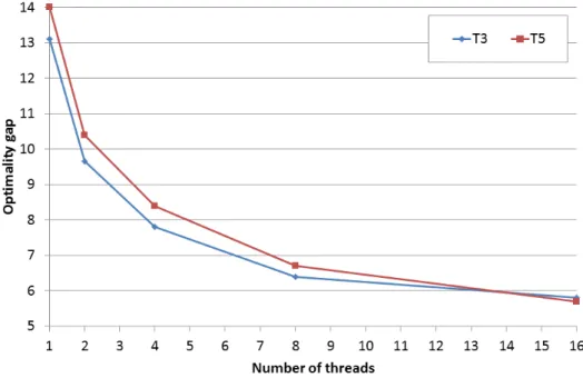
Figure 1: CPLEX average relative optimality gap (%) with respect to the number of parallel threads
Initial experiments on the T3 and T5 instance sets showed ∆CP figures greater than
10% after 24 hours of execution. This underlined the difficulty of even very good com-mercial MIP solvers such as CPLEX to solve even limited-size problem instances. The high degree of symmetry inherent to the problem contributes to this difficulty.
We therefore used CPLEX in parallel mode. Figure 1 shows the trend of the average relative optimality gap for T3 and T5 instances with respect to the number of parallel threads. The gap decreases rapidly as the number of threads increases. With 16 parallel threads, CPLEX has an average optimality gap below 6%. The results of parallel CPLEX with 16 threads are therefore used in the comparisons of this section.
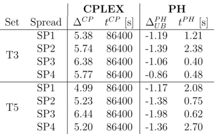
Table 1 details the comparison of CPLEX and the PH meta-heuristic for the T3 and T5 instances; CPLEX was unable to solve T10 with a reasonable optimality gap. We report, for each combination of instance set (Column 1) and item spread class (Column 2), the average optimality gaps ∆CP of CPLEX (Column 3), the average running times
tCP of CPLEX (Column 4), the average running timestP H of the meta-heuristic (Column
6), and, in Column 5, the average gaps ∆P H
U B of the meta-heuristic computed as
∆P HU B = U B
P H −U BCP
U BCP , (6.5)
where U BP H is the objective value of the meta-heuristic. Note that the value of ∆P HU B may be positive or negative. When ∆P H
U B is negative, the meta-heuristic solution is better
CPLEX PH Set Spread ∆CP tCP [s] ∆P HU B tP H [s] T3 SP1 5.38 86400 -1.19 1.21 SP2 5.74 86400 -1.39 2.38 SP3 6.38 86400 -1.06 0.40 SP4 5.77 86400 -0.86 0.48 T5 SP1 4.99 86400 -1.17 2.08 SP2 5.23 86400 -1.38 0.75 SP3 6.44 86400 -1.98 0.62 SP4 5.20 86400 -1.36 2.70
Table 1: Comparison of CPLEX and PH-based meta-heuristic
As stated before, CPLEX cannot solve the SVCSBPP to optimality within a reason-able time limit for any instance considered. The average optimality gap after 24 hours is always greater than 5%, with a maximum value of 6.44%. The PH meta-heuristic is accurate and effective on all T3 and T5 instances. It always converges quickly to better solutions than those obtained by CPLEX. The gap ∆P H
U B is negative for all instances
with an average improvement in the solution values between 0.86% and 1.98%. The PH meta-heuristic always reaches a consensus solution in less than 3 s. This performance is directly related to the efficiency of the heuristic solver for the VCSBPP, which is able to solve deterministic subproblems in negligible computational times.
Despite the use of concurrent computation, CPLEX is not able to identify a good feasible solution for T10 instances in 24 h of computing time. These instances can easily involve more than 10 million variables. They require a huge amount of memory for the branch and bound (e.g., more than 64 GB of memory already occupied after 2 h of computation). Memory thus rapidly becomes a bottleneck, and CPLEX cannot run for the assigned time. Thus, to validate the PH meta-heuristic on the remaining instances, we compare its solutions with those obtained by solving the LB (4.1)–(4.4). Recall that the LB does not consider item-to-bin assignments, which drastically reduces the number of variables in the model. The reduced model can thus be solved to optimality by CPLEX with a limited computational effort. The time depends on the number of bins involved, so CPLEX requires only a few seconds to solve LB for sets T3, T5, and it needs at most 120 s for set T10.
Table 2 reports, for each instance set (Column 1) and item spread class (Column 2), the percentage gap ∆P HLB between the objective function value obtained by the PH meta-heuristic and LB (Column 3), and the average and maximum percentage increase in the objective function value (Columns 4 and 5) resulting from the use of the LB solutions as the capacity plan. On average, the gaps are smaller than 2%, underlining the accuracy of the PH meta-heuristic. We further qualified this accuracy by evaluating the quality of the LB solutions by fixing the bin selections defined by LB and computing the recourse
Set Spread ∆P H LB CLB CmaxLB T3 SP1 0.88 0.21 1.45 SP2 0.72 0.22 1.79 SP3 0.68 0.05 0.45 SP4 1.21 0.00 0.00 T5 SP1 1.57 0.09 0.63 SP2 1.45 0.00 0.00 SP3 1.03 0.06 0.47 SP4 2.03 0.10 0.77 T10 SP1 0.81 0.04 0.31 SP2 0.79 0.03 0.18 SP3 0.76 0.02 0.19 SP4 0.86 0.01 0.06 Table 2: Comparison of LB and PH solutions
cost. For instances T3, T5, and T10, the average increase in the objective function was smaller than 0.25%,.No increase,CLB = 0, was observed in a number of cases, signaling
that the capacity plans defined by LB and the PH meta-heuristic match exactly.
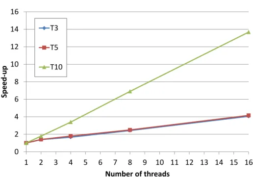
We conclude this section by analyzing the scalability of the parallel implementation of the meta-heuristic with up to 16 threads. The computational wall-clock timestP H for
each instance set (Column 1) and item spread class (Column 2) are reported in Table 3 for 1, 2 , 4, 8 and 16 threads. The average speedups for the three instance sets, defined as the ratio of the sequential running time to the parallel running time, are displayed in Figure 2.
Computational times are negligible for T3 and T5 instances, while becoming more significant for the larger instances, the computational effort increasing with the number of items and especially with the number of bin types (e.g., instances in T10). Yet, the maximum sequential time of the meta-heuristic, of the order of 600 wall-clock seconds, is still several orders of magnitude smaller than the time required by CPLEX.
The scaling of the master-slave parallel implementation is quite linear. The speedups are of the order of 4 with 16 parallel threads for T3 and T5 instances, while they reach almost 14 (80% of the linear speedup) for T10 instances. Recalling that the VCSBP-Pheuristic is very fast on all instances (which results in a balanced workload for slaves), the results indicate that for parallel computation is not really required for the small instances (and certainly not 16 threads; 4 are giving a 50% speedup), most time being spent on exchanging information between the master and the slaves. Parallel computing becomes appropriate as dimensions grow, which indicates that large problem instance can be addressed efficiently with the proposed methodology.
Set Spread tP H1 tP H2 tP H4 tP H8 tP H16 T3 SP1 1.21 0.87 0.73 0.50 0.30 SP2 2.36 1.73 1.41 0.97 0.59 SP3 0.41 0.29 0.25 0.17 0.10 SP4 0.49 0.35 0.29 0.20 0.12 T5 SP1 2.08 1.48 1.15 0.83 0.50 SP2 0.75 0.53 0.42 0.30 0.18 SP3 0.62 0.44 0.35 0.25 0.15 SP4 2.70 1.93 1.50 1.08 0.65 T10 SP1 625.17 350.10 187.08 89.02 45.62 SP2 580.59 325.52 174.53 85.05 42.56 SP3 432.48 241.24 122.87 74.25 31.52 SP4 524.87 293.35 155.24 75.85 38.47
Table 3: Average computational times for the meta-heuristic with respect to parallel threads 0 2 4 6 8 10 12 14 16 1 2 3 4 5 6 7 8 9 10 11 12 13 14 15 16 Speed -up Number of threads T3 T5 T10
6.3
Benefit of modeling the uncertainty
The question addressed in this section is whether modeling uncertainly explicitly through the SVCSBPP two-stage model with recourse is warranted compared to solving some deterministic variant of the problem. We address this question by comparing the results of the stochastic formulation RP, to those of thewait and see,WS, andexpected value,EV, problems, respectively. The well-known stochastic programming measures, the expected value of perfect information, EVPI, and the value of the stochastic solution,VSS (Birge, 1982; Maggioni and Wallace, 2012).
The EVPI is defined as the difference between the objective values of the stochastic solution and that of the wait-and-see problem
EV P I :=RP −W S, (6.6) the latter problem being defined by assuming the realizations of all the random parame-ters are known at the first stage.
The VSS indicates the expected gain from solving the stochastic model rather than its deterministic counterpart in which the random parameters are replaced with their expected values:
V SS :=EEV −RP, (6.7)
where, in our case, EEV denotes the solution value of EV, the stochastic model with the first-stage decision variables fixed at the optimal values obtained by using the expected values of the coefficients.
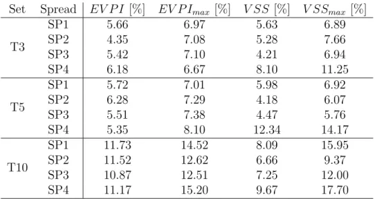
We present aggregated results in Table 4, grouped by instance set (Column 1) and spread class (Column 2). The table reports, the average and maximum EVPI percentages (Columns 3 and 4), computed as EV P I/RP ·100, and the average and maximum VSS percentages (Columns 5 and 6) computed as V SS/RP ·100.
The EVPI percentage is around 10%, showing the benefit of having information about the future in advance. It increases with the problem dimensions to a maximum value above 15%. The average and maximum values of VSS also increase as the size of the instance increases. The gap between the expected-value solution and the stochastic solution is significant for all sets considered. Even for small instances, the maximum VSS reaches 11%, emphasizing the potential loss incurred by following the capacity plan of the deterministic solution. The most critical item spread class is SP4, representing the case when no information is available about the category distribution of the items to be shipped. It is therefore the most representative instance class for the shipping freight over long distances, and it displays a maximum EVPI of 15.20%, with a maximum VSS always greater than 7% and reaching 17.70%. We therefore conclude that using the stochastic model is appropriate and beneficial.
Set Spread EV P I [%] EV P Imax [%] V SS [%] V SSmax [%] T3 SP1 5.66 6.97 5.63 6.89 SP2 4.35 7.08 5.28 7.66 SP3 5.42 7.10 4.21 6.94 SP4 6.18 6.67 8.10 11.25 T5 SP1 5.72 7.01 5.98 6.92 SP2 6.28 7.29 4.18 6.07 SP3 5.51 7.38 4.47 5.76 SP4 5.35 8.10 12.34 14.17 T10 SP1 11.73 14.52 8.09 15.95 SP2 11.52 12.62 6.66 9.37 SP3 10.87 12.51 7.25 12.00 SP4 11.17 15.20 9.67 17.70
Table 4: EVPI and VSS comparison
We complete this section by examining to what extent the first-stage decisions differ between the stochastic and the EV formulations. On average, the EV problem overesti-mates the demand to be loaded (the total volume of the items is larger than the actual volume) and the availability of extra bins (a larger set of bins is available for the recourse action). This can lead to two situations. On the one hand, EV may plan to use a larger set of bins that is not actually required, given the set of scenarios considered. The ca-pacity plan is then more expensive (i.e., the cost increases by 17.70%), but the solution is feasible. ON the other hand, EV may plan an insufficient capacity for a subset of scenarios in which the actual availability of bins is very limited. The capacity plan is infeasible for these scenarios. This case is rare, occurring for only 2% of the instances. In both cases, the results clearly show the need to explicitly consider uncertainty in capacity-planning applications.
6.4
Solution analysis
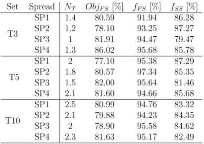
We focus on the structure of the capacity-planning solutions and in particular on the use of bins in the plan. Table 5 reports, for each combination of instance set (Column 1) and item spread class (Column 2), the average number of bin types NT used in the
capacity plan (Column 3), the percentage of the objective function value achieved in the first stage ObjF S (Column 4), and the average fill level of the bins (as a percentage of
capacity) at the two stages, fF S and fSS respectively (Columns 5 and 6).
It is noticeable that only a few bin types are used in the plan. The number is close to 1 for T3 instances, and it is between 2 and 3 for instances in sets T5 and T10, which have five and ten bin types, respectively. Furthermore, the number of bins is not evenly
Set Spread NT ObjF S [%] fF S [%] fSS [%] T3 SP1 1.4 80.59 91.94 86.28 SP2 1.2 78.10 93.25 87.27 SP3 1 81.91 94.47 79.47 SP4 1.3 86.02 95.68 85.78 T5 SP1 2 77.10 95.38 87.29 SP2 1.8 80.57 97.34 85.35 SP3 1.5 82.00 95.64 81.46 SP4 2.1 81.60 94.66 85.68 T10 SP1 2.5 80.99 94.76 83.32 SP2 2.1 79.88 94.23 84.35 SP3 2 78.90 95.58 84.62 SP4 2.3 81.63 95.17 82.49 Table 5: Structure of solutions
distributed among the types. Almost all of the bins included in the capacity plan are of the same type; only one or two bins are of different types. Concerning the spread classes, it is interesting to note that, when the stochastic problem considers a demand with a high percentage of small items (classes SP1 and SP4), NT is maximum. In fact,
small items may be loaded into any bins (large items cannot be placed into bins with limited capacities), and they are usually used to fill near-empty bins. Thus, it becomes attractive for the model to mix bin types.
The percentage of the objective function coming from the first stage planning decisions is of the order of 80%. This indicates interest for tactical decisions to be conservative: the company should book sufficient capacity in advance to limit the adjustments necessary when the actual demand becomes known. This also indicates that 10%-20% of plan adjustment (recourse) is a good compromise between cost reduction and uncertainty management.
Finally, the fill levels of the bins selected during the first and second stages are over than 90% and 70%, respectively. This indicates the effectiveness of the capacity plan, which uses the contracted bins at almost full capacity and requires only limited adjust-ments at the second stage.
6.5
Sensitivity analysis
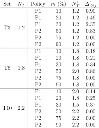
We now turn to the sensitivity of the problem and the proposed logistics capacity plan to limits on the availability of bins coming, e.g., from contractual policies imposed by the 3PL. We analyze the issue through two policies. The first policy (P1) imposes a
minimum number of bins for each bin type τ included in the capacity plan. The second policy (P2) reduces the number of available bins of each type, which requires the plan to combine different types of bins in the most efficient way.
Set NT Policy m (%) NT0 ∆0Obj
T3 1.2 P1 10 1.2 0.90 P1 20 1.2 1.46 P1 30 1.2 2.35 P2 50 1.2 0.83 P2 75 1.2 0.00 P2 90 1.2 0.00 T5 1.8 P1 10 1.8 0.18 P1 20 1.8 0.21 P1 30 1.8 0.34 P2 50 2.0 0.86 P2 75 1.8 0.00 P2 90 1.8 0.00 T10 2.2 P1 10 2.0 0.14 P1 20 1.8 0.25 P1 30 1.5 0.37 P2 50 2.2 0.00 P2 75 2.2 0.00 P2 90 2.2 0.00
Table 6: Sensitivity of capacity planning to bin availability
Let uτ =kJτk be the number of bins of type τ that can be selected for the capacity
plan. We define the minimum number of bins to be m·uτ, with m={10%,20%,30%}.
Similarly, the maximum availability is reduced to m·uτ with m={0.50,0.75,0.80}. To impose these policies, we introduce into the formulation the additional constraints (6.8) for the first policy, and (6.9) for the second policy:
X j∈Jτ yτ sj ≥m·uτ ∀τ ∈ T, s ∈ S (6.8) X j∈Jτ yjτ s ≤m·uτ ∀τ ∈ T, s∈ S. (6.9)
We compare the results of the PH meta-heuristic for the two policies and those of the original formulation. Table 6 reports the average results of the sensitivity analysis for each set of instances (Column 1), the original number of bin types used in the plan NT
(Column 2), the policy type (Column 3), and the associated value of factor m (Column 4). For each policy, we show the changes in the solutions with respect to the number of bin types used (NT0 , Column 5) and the extra cost for the policy (∆0Obj, Column 6).
We note that the instances with a limited availability of bin types (T3) are more sensitive to policy P1. For these sets, P1 penalizes combinations of bin types, causing an increase in the cost of the first-stage capacity plan or in the recourse action contracting more bins. This cost increases as the number of bin types available decreases, e.g., it is approximately 2% for instances T3. Similarly, P1 tends to penalize the use of bin types for T5 and T10, but the impact on the objective function is limited. The wide choice of bins that characterizes these instances allows them to efficiently implement the policy, reducing the cost associated with the second stage.
P2 reduces the set of bins available at planning time. Thus, it is necessary to combine the available bins for each type (replacing the large bins that cannot be selected with more smaller bins). The policy becomes significant only in extreme cases in which the original availability of the bins is halved (e.g., m = 50%). The solutions then include more bins, resulting in a higher fixed cost. The effect of this policy is very limited, however, with an increase in objective function of 0.86%. In the worst case, when the plan does not meet the demand, the recourse selects extra capacity at a premium cost.
6.6
Long-term behavior of capacity plan
The goal of this analysis is to evaluate the robustness and reliability of the capacity planning decisions when the demand moves significantly away from the distribution and the estimation (reflected in the set of scenariosS). This situation can be observed when economic conditions change significantly resulting in higher and lower demands.
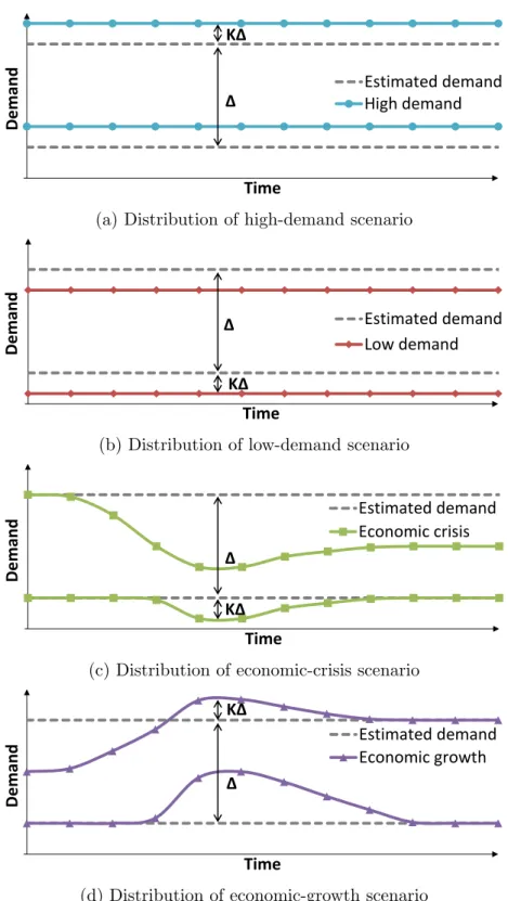
We performed Monte Carlo simulations (on a 10% subset of the instances) for a relatively long period (1 year) for four demand scenarios:
1. High demand (Figure 3a illustrates the range of the demand in this scenario
relative to the initial one): The average demand is higher than the demand of the scenarios inS. This case aims to measure the cost of overusing the spot market to obtain the extra capacity.
2. Low demand(Figure 3b): The average demand is lower than the demand of the
scenarios in S. This case focuses on the cost of not using part of the planned capacity.
3. Economic crisis(Figure 3c): The demand decreases rapidly to a value below the
estimated demand. It then stabilizes below the average demand of the scenarios in
S.
4. Economic recovery (Figure 3d): The demand is initially below the average
esti-mated demand, but it increases rapidly to a peak above the maximum estimation. It then stabilizes.
D e mand Time Estimated demand High demand Δ KΔ
(a) Distribution of high-demand scenario
D e mand Time Estimated demand Low demand KΔ Δ
(b) Distribution of low-demand scenario
D e mand Time Estimated demand Economic crisis Δ KΔ
(c) Distribution of economic-crisis scenario
D e mand Time Estimated demand Economic growth Δ KΔ
(d) Distribution of economic-growth scenario
The overall simulation process was:
Given an instance and the associated set of scenarios S, find the capacity-planning solution using the PH meta-heuristic.
Create a new set of scenarios S0:
– Identify the maximum and minimum demand inS and compute the difference ∆ between them.
– ComputeK∆ for the current demand scenario, whereK ={10,20,30,40,50}% is an offset factor that defines how far the demand distribution has to be from that estimated in set S (Figure 3).
– Define 365 scenarios respecting the trends of the demand and the characteris-tics of the instance (number of bin types and spread class of items).
For each scenario s ∈ S0, build a VCSBPP with the bin set formed by the bins
included in the capacity-planning solution and the bins at premium cost defined in the scenario, and the demand in terms of the items to be loaded. The resulting VCSBPP is then solved by the meta-heuristic.
Given the solution, compute the expected value of the total cost and statistics related to the use of the planned bins and of the extra capacity required to cover higher demand, and the corresponding cost.
Repeat 10 times and average the results.
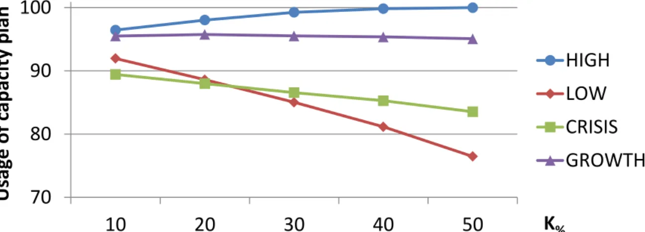
Figure 4 shows the results of the Monte Carlo simulation for an illustrative instance from set T10 (the other instances produced similar results). The figure reports, for each demand scenario, the usage percentage of the logistics capacity plan, defined as the ratio of the number of planned (selected in the first stage) bins actually used in the solution to the total number of bins selected in the plan (Figure 4a), the percentage of extra bins in the solution defined as the ratio of the number of extra bins to the total number of bins in the solution (Figure 4b), and the percentage of the objective function value associated with the capacity plan (Figure 4c), with respect to the offset factor K.
Despite the high variability of the stochastic parameters in instances T10, the capacity-planning decisions appear valid. Increasing the offset factorK increases or decreases the percentage of the planned capacity actually used according to the demand trend in differ-ent demand scenarios. Thus, for the LOW and CRISIS scenarios, the use of the planned bins decreases, to an average of 77% for T10 instances in the worst case. In contrast, for the HIGH and GROWTH scenarios, the number of planned bins actually used in the solution is always greater than 90%. The reduction in the planned capacity used in the LOW and CRISIS scenarios parallels a decrease in the need for extra capacity. This is particularly evident for T10 instances, for which no extra capacity is needed when the
70
80
90
100
10
20
30
40
50
Usag
e
o
f
capac
ity
p
la
n
K
%HIGH
LOW
CR
I
SIS
GROWTH
(a) Percentage of planned (first-stage) bins actually used in the solution
0
5
10
15
20
25
10
20
30
40
50
Extr
a
capac
ity
K
%HIGH
LOW
CR
I
SIS
GROWTH
(b) Percentage of extra bins in the solution
70
75
80
85
90
95
100
10
20
30
40
50
FS
Objectiv
e
fu
n
ctio
n
K
%HIGH
LOW
CR
I
SIS
GROWTH
(c) Objective function value associated with the capacity plan
demand is minimum (LOW scenario and K = 50%). Conversely, when the demand is underestimated, it may be necessary to purchase additional capacity; more than 20% for the HIGH scenario (some 7 bins for T10 instances) and between 10% and 15% for the GROWTH scen