Fast Statistical Spam Filter by Approximate Classifications
Kang Li
Department of Computer Science University of Georgia Athens, Georgia, USA
Zhenyu Zhong
Department of Computer Science University of Georgia Athens, Georgia, USA
ABSTRACT
Statistical-based Bayesian filters have become a popular and important defense against spam. However, despite their ef-fectiveness, their greater processing overhead can prevent them from scaling well for enterprise-level mail servers. For example, the dictionary lookups that are characteristic of this approach are limited by the memory access rate, there-fore relatively insensitive to increases in CPU speed. We address this scaling issue by proposing an acceleration tech-nique that speeds up Bayesian filters based on approximate classification. The approximation uses two methods: hash-based lookup and lossy encoding. Lookup approximation is based on the popular Bloom filter data structure with an ex-tension to support value retrieval. Lossy encoding is used to further compress the data structure. While both methods introduce additional errors to a strict Bayesian approach, we show how the errors can be both minimized and biased toward a false negative classification. We demonstrate a 6x speedup over two well-known spam filters (bogofilter and qsf) while achieving an identical false positive rate and sim-ilar false negative rate to the original filters.
Categories and Subject Descriptors
C.4 [Computer Systems Organization]: Performance attributes; H.4 [Information Systems Applications]: Mis-cellaneous
General Terms
Algorithms, Performance
Keywords
SPAM, Bloom Filter, Approximation, Bayesian Filter
1.
INTRODUCTION
In recent years, statistical-based Bayesian filters [13, 21, 23], which calculate the probability of a message being spam
Permission to make digital or hard copies of all or part of this work for personal or classroom use is granted without fee provided that copies are not made or distributed for profit or commercial advantage and that copies bear this notice and the full citation on the first page. To copy otherwise, to republish, to post on servers or to redistribute to lists, requires prior specific permission and/or a fee.
SIGMetrics/Performance’06, June 26–30, 2006, Saint Malo, France. Copyright 2006 ACM 1-59593-320-4/06/0006 ...$5.00.
based on its contents, have found wide acceptance in tools used to block spam. These filters can be continually trained on updated corpora of spam and ham (good email), resulting in robust, adaptive, and highly accurate systems.
Bayesian filters usually perform a dictionary lookup on each individual token and summarize the result in order to arrive at a decision. It is not unusual to accumulate over 100,000 tokens in a dictionary, depending on how training is handled [23]. Unfortunately, the performance of these dic-tionary lookups is limited by the memory access rate, there-fore relatively insensitive to increases in CPU speed. As a result of this lookup overhead, classification can be relatively slow. Bogofilter [23], a well-known, aggressively optimized Bayesian filter, processes email at a rate of 4Mb/sec on our reference machine. According to a previous survey on spam filter performance [15], most well-known spam filters, such as SpamAssassin [27], can only process at about 100Kb/sec. This speed might work well for personal use, but it is clearly a bottleneck for enterprise-level message classification.
The goal of our work is to invent techniques to speed up spam filters while keeping high classification accuracy. Our overall approach uses approximate classifications, which allows us to move the bottleneck from memory access time to CPU cycle time, thus allowing for better scalability as CPU performance improves.
The first of our two methodsapproximates the dictionary lookup with hash-based Bloom filter [3]lookup, which trades off memory accesses for an increase in computation. Bloom filters have recently been used in computer network tech-nologies ranging from web caching [11], IP traceback [28], to high speed packet classifications [5]. While Bloom fil-ters are good for storing binary set membership information, statistical-based spam filters need to support value retriev-ing. To address this limitation, we extended Bloom filters to allow value retrieval and explored its impact on filter ac-curacy and throughput. Our second approximation method useslossy encoding, which applies lossy compression to the statistical data by limiting the number of bits used to rep-resent them. The goal is to increase the storage capacity of the Bloom filter and control its misclassification rate.
Both approximations by Bloom filter and lossy encoding introduce a risk of increasing the filter’s classification error. We investigate the tradeoff between accuracy and speed, and present design choices that minimize message misclas-sification. Furthermore, we propose methods to ensure that misclassifications, if they do occur, are biased towards false negatives rather than false positives, as users tend to have much less tolerance for false positives.
This paper presents analytical and experimental evalu-ations of the filters using these approximation techniques, collectively, known as Hash-based Approximate Inference (HAI). The HAI filter implementations in this paper are based on the popular spam filters bogofilter [23] and qsf [30], and the improved filters have shown a factor of 6x speedup with similar false negative rates (7% more spam) and iden-tical false positive rate compared to the original filters.
The scope of this paper is limited to optimizing the pro-cessing speed of a particular anti-spam filter and preserving its current classification accuracy. Difficulties and limita-tions [19, 29] with the general statistic-based anti-spam ap-proach are beyond the scope of this paper.
The rest of the paper is organized as follows: Section 2 reviews a normal Bayesian filter and the algorithm that it uses to combine token statistics in order to compute an overall score. Section 2 also reviews the concept of hash-based lookup using Bloom filters. Section 3 describes the architecture of the HAI filters and the two approximation methods, and explores their potential impact to the filter-ing results. Section 4 presents our experimental evaluation results of HAI filters. The paper ends with related work and concluding remarks in Section 5 and 6, respectively.
2.
BACKGROUND
To provide the necessary background information for the discussion of the filter acceleration technique, we first review the normal classification process for Bayesian filters and de-scribe the basic concept of Bloom filters.
2.1
Naive Bayesian Based Filter
Bayesian probability combination has been widely used in various message classifications. To make a classification, a message is first parsed into tokens (words or phrases), and the frequencies of tokens shown in previously known types (spam or ham) are obtained. Based on the combination of all individual token’s frequency statistics, the message is classified into one or more categories. Here, only two cate-gories are necessary: spam or ham. Almost all the statistic-based spam filters use Bayesian probability calculation [14] to combine individual token’s statistics to an overall score, and make filtering decision based on the score.
Usually, these filters first go through a training stage that gathers statistics of each token. The statistic we are mostly interested for a token T is its spamminess, calculated as follows:
S[T] = Cspam(T) Cspam(T) +Cham(T)
(1) where Cspam(T) andCham(T) are the number of spam or
ham messages containing tokenT, respectively.
To calculate the possibility for a messageM with tokens
{T1, ..., TN}, one needs to combine the individual token’s
spamminess to evaluate the overall message spamminess. A simple way to make classifications is to calculate the product of individual token’s spamminess (S[M] = Ni=1S[Ti]) and
compare it with the product of individual token’s hammi-ness (H[M] = N
i=1(1−S[Ti])). The message is considered
spam if the overall spamminess productS[M] is larger than thehamminessproductH[M].
The above description is used to illustrate the idea of statistic based filters using Bayesian classifications. In prac-tice, various techniques are developed for combining token
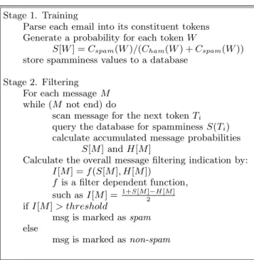
Stage 1. Training
Parse each email into its constituent tokens Generate a probability for each tokenW
S[W] =Cspam(W)/(Cham(W) +Cspam(W))
store spamminess values to a database Stage 2. Filtering
For each messageM while (M not end) do
scan message for the next tokenTi
query the database for spamminess S(Ti)
calculate accumulated message probabilities S[M] andH[M]
Calculate the overall message filtering indication by: I[M] =f(S[M], H[M])
f is a filter dependent function, such as I[M] = 1+S[M]−H[M] 2 ifI[M]> threshold msg is marked asspam else msg is marked asnon-spam
Figure 1: Outline for A Bayesian Filter Algorithm
probabilities to enhance the filtering accuracy. For exam-ple, many Bayesian filters, including bogofilter and qsf, use a method suggested by Robinson [25]: Chi-squared prob-ability testing. The Chi-squared test calculates S[M] and H[M] based on the distribution of all the tokens’ spammi-ness (S[T0], S[T1], ...}) against a hypothesis, and scaleS[M]
andH[M] to a range of 0 to 1. Details of this algorithm are described in [23, 25],
To avoid making filtering decision whenH[M] andS[M] are very close, several spam filters [21, 23, 30] calculate the following indicator instead of comparing H[M] and S[M] di-rectly
I[M] =1 +S[M]−H[M]
2 (2)
WhenI >0.5, it indicates the corresponding message has a higher spam probability than ham probability, and should be classified accordingly. In practice, the final filter result is based onI > thresh, wherethreshis a user selected thresh-old. For conservative filtering,threshis a value closer to 1, which will filter fewer spam messages, but is less likely to result in false positives. Asthresh gets smaller, the filter becomes more aggressive, blocking more spam messages but also at a higher risk of false positives. A general Bayesian filter algorithm is presented in Figure 1. It is first trained with known spam and ham to gather token statistics and then classifies messages by looking at its token’s previously collected statistics. A more detailed description of Bayesian spam filter algorithm can be found in several recent publi-cations [1, 13, 21, 23].
2.2
Bloom Filters
A Bloom filter is a compact data structure designed to store query-able set membership information [3]. Bloom filters were invented by Burton H. Bloom to store large amounts of static data such as English hyphenation rules.
0 1 0 1 1 H1 H2 TOKEN H3 Hash Functions (m bits) Bit Vector
Figure 2: Training A Bloom Filter
A Bloom filter consists of a bit vector of length m that represents the set membership information about a dictio-nary of tokens. The filter is first populated with each mem-ber (token) of the set (Figure 2 shows a Bloom filter in this training phase). At the training phase, for each token in the membership set,h hash functions are computed on the token producing h hash values each ranging from 1 to m. Each of these hash values addresses a single bit in the m-bit vector, and sets that bit to 1. Hence for perfect hashes, each token causes h bits of the m-bit vector to be set to 1. In the case that a bit has already been set to 1 because of hash conflicts, that bit is not changed.
Querying a token’s membership is similar to the training process. Figure 3 shows a Bloom filter in the query stage with a non-member token. For a given token,hhash results are produced and each addresses one bit. The token is guar-anteed not in the set if any of these bits is not set to 1. If all theh bits are set to 1, the token is said to belong to the set. This claim is not always true because the fact of these
h bits being 1 could be a result of the hashes of multiple other member tokens. This case is considered to be a false positive for membership testing.
The likelihood of false positive occurrence can be made very small by carefully choosing the size of bit vector and number of hash functions. We illustrate this with a brief overview of the false positive probability derivation:
Assuming perfect hash functions and a m-bit vector, the probability of setting a random bit to 1 by one hash is 1/m, and thus the probability that a bit is not set by a single hash function is (1−1/m). Forhhash functions, the probability that a bit is not set by any of the hashes is (1−1/m)h. For
a member set withntokens, the probability of a bit not set is
P0= (1− 1 m)
n∗h
(3) and the probability of a bit set to 1 is
P1= 1−(1− 1 m)
n∗h
(4) For a non-member token to be misclassified as a possible set member, all theh bits addressed byh hash functions
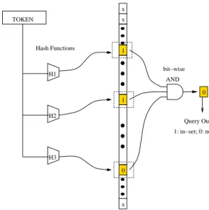
x x 1 1 x 0 0 H1 H2 TOKEN H3 Hash Functions AND bit−wise Query Output Bit Vector 1: in−set; 0: not−in−set (m bits)
Figure 3: Query A Bloom Filter
must be 1. Thus the probability of a false positive is
Pm,n,h(fpos) = (1−(1−
1
m)
n∗h)h (5) Note that the above probability is the false positive for token membership testing, which isvery different from the false positive of email message classification. The latter usu-ally combines multiple tokens’ spamminess values in order to arrive at a probability result. The next section discusses how to control the effect of the Bloom filter misclassification to minimize the email message misclassifications.
3.
OUR APPROACH
This section describes the architecture of the HAI filter as well as an extension to Bloom filters in order to support value retrieval queries.
3.1
Extending Bloom Filter for Value Retrieval
Traditional Bloom filters only make membership queries that verify whether a given token is in a set, but applications such as spam filters must retrieve each token’s associated probability value. We extend the Bloom filter to serve for value queries while preserving Bloom filter’s desired original operating characteristics. For a given token in the member set, the extension returns a value that corresponds to a given token.
The idea of this extension is to simply maintain a two-dimensional vector, which has a total bit-vector size of m bits, and every hash output points to one of ther entries, each of which has q bits (i.emis the product ofr and q). The traditional Bloom filter becomes a special case of this extension that uses one bit per entry (q=1).
Figure 4 shows the structure of this Bloom filter exten-sion. It works in the following way to support value retrieval. During the Bloom filter training phase, each training to-ken runs through the hash functions and addresseshentries (each entry containsqbits). Assume the token has an asso-ciated value (in integer)v in a range of 0 toq−1. The value vis then stored to the Bloom filter extension by setting the
x x x x x x x x x x x x 0 0 1 0 1 0 1 0 1 0 0 1 0 0 1 0 q bits H1 H2 TOKEN H3 Hash Functions AND bit−wise
Query Output Value Decoder Multi−bit Vector
(m=r*q bits)
Figure 4: Bloom Filter Extension for Value Retriev-ing Query (The Bit-Vector hasr entries and q bits per entry)
vth-bit to 1 on all thesehentries. During the query phase, each incoming token also goes through the hashing and ad-dresseshentries. The query outcome for this token is based on the logical AND of allhentries. If none of the bits is set in the logical AND output, it indicates that the token in the query is not in the training set. If a bit is set, then based on the position of the bit, we retrieve the value associated with the token. The accuracy of this Bloom filter extension as well as its application in HAI filter are discussed in the next subsection.
3.2
HAI Filter Architecture
We build HAI spam filter based on this Bloom filter ex-tension. The HAI filter is used in the same way as normal Bayesian filters: first a training phase that store the statis-tics from known spam and ham; then a query phase that classifies messages by running lookups for the incoming to-kens through the stored statistics. The HAI filter’s archi-tecture differs from the normal filters by the representation and consequently the query of the statistical data. The HAI filter algorithm is presented in Figure 5.
3.2.1
Approximation by Quantization
To effectively use the Bloom filter extension for approx-imate value retrieval queries, we introduce lossy encoding (quantization) to represent the individual token’s spammi-ness value. Consider the way that the Bloom filter extension represents a statistical value by marking one bit of aq-bit entry. It has to adopt some quantization technique if the amount of potential numbers to be represented is infinite.
During the training phase, each tokenT obtains a proba-bility valuepbased on it shows up in ham and spam. HAI differs from traditional Bayesian filter by mapping a token’s probability valuepto an integer valuevbetween 0 andq−1,
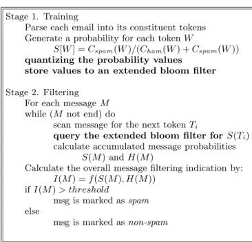
Stage 1. Training
Parse each email into its constituent tokens Generate a probability for each tokenW
S[W] =Cspam(W)/(Cham(W) +Cspam(W))
quantizing the probability values store values to an extended bloom filter
Stage 2. Filtering For each messageM while (M not end) do
scan message for the next tokenTi
query the extended bloom filter forS(Ti)
calculate accumulated message probabilities S(M) andH(M)
Calculate the overall message filtering indication by: I(M) =f(S(M), H(M))
ifI(M)> threshold
msg is marked asspam
else
msg is marked asnon-spam
Figure 5: HAI Filter Algorithm (Highlights are changes made to Bayesian filters)
where qis a parameter of the Bloom filter extension called the quantization level. The token is then considered to be associated with valuev for storing and retrieving with the Bloom filter extension. When used at the end to calculate a message’s spamminess, a token’s probability valuev is ap-proximately mapped back topbased on the quantization.
This paper studies the effect of different quantization lev-els on Bloom filter’s lookup performance. Two aspects of quantization effects need to be addressed. First, we would like to choose an optimal quantization level (q), which af-fects both the size (m) of the Bloom filter’s bit-vector and the Bloom filter misclassification rate. The latter is dis-cussed in the next subsection.
Second, for each given quantization level, we would like to pick the optimal mapping between the values to be quan-tized and the values after quantization for minimal errors. This paper uses Lloyd-Max algorithm [20] to obtain the op-timal quantizer for the token spamminess values for each given quantization level. The Lloyd-Max algorithm is bor-rowed from previous studies of optimal quantization (such as those used in MPEG [12]) in the area of lossy encoding [2]. It is one of the popular algorithms that make a non-uniform optimal quantization that provides minimal “quality distor-tion” to videos.
3.2.2
Approximate Lookup
This extension allows the Bloom filter to support value re-trieval queries at a cost of higher error rate compared to the original Bloom filter. Two types of misclassification could happen in this extended Bloom filter.
First, similar to the original Bloom filter, the extended one could misclassify a non-member token as a member and mistakenly provide a value. The chance of such false positive misclassification increases because if any bit of the multi-bit output entry is set to one by hash conflicts, a false positive will occur. To derive the probability of this false positive,
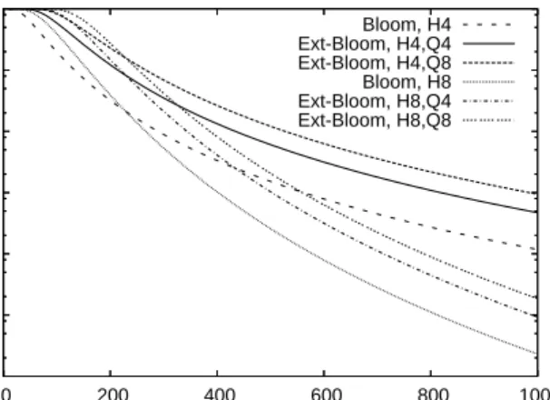
1e-06 1e-05 1e-04 0.001 0.01 0.1 1 0 200 400 600 800 1000
Token Misclassification Probability
Bloom Filter Size (KBytes)
Dictionary=220,000 Tokens; H: Hash; Q: Quantization Bloom, H4 Ext-Bloom, H4,Q4 Ext-Bloom, H4,Q8 Bloom, H8 Ext-Bloom, H8,Q4 Ext-Bloom, H8,Q8
Figure 6: Lookup Error Rate vs. Bit-vector Sizes
let us first only consider a single bit of the query outcome. From the single dimension Bloom filter (Equation 5), we can derive that the possibility for a single bit being zero as
Pm,n,h(0) = 1−Pm,n,h(fpos) = 1−(1−(1−
1
m)
n∗h)h (6) With the final logical AND output havingqbits, the pos-sibility of false positive becomes
Pm,n,h,q(fpos) = 1−(Pm,n,h(0))q (7)
Second, a new type of error occurs when more than one bits of the final Bloom filter outcome are set to 1. The prob-ability of a multi-bit marking is equivalent to one minus the probability of all bits being set to zero and the probability of only one bit getting 1.
Pm,n,h,q(multi) = 1−(Pm,n,h(0))q−q∗(1−Pm,n,h(0))(q−1)
(8) The probability rates for both types of errors depend on the number of tokens (n), the Bloom filter bit-vector size (m), the number of hash functions (h), and the quantization level (q). Figure 6 shows a theoretical error rate for a dic-tionary with 220,000 tokens versus various bit-vector sizes from 0 to 1 MB, 4 or 8 hash functions, and 4 or 8 bits quan-tization respectively. The dictionary size is selected based on the recommended token sizes by [23]. The results indi-cate that the selection of Bloom filter parameters (m,h,q) affects the misclassification rate significantly. For a small number of hash functions, the Bloom filter can reach less than a 0.1% token misclassification rate with less than 1MB memory under small quantization levels (4 or 8 bits in this example).
3.3
Control the Filter Accuracy
This section discusses how to reduce the total errors caused by the two approximations (quantization and approximate lookup) in order to limit their impact to the final message classification errors. We control the impact of these errors by choosing appropriate Bloom filter size and quantization level that minimize the total lookup errors. In the case of multi-bit marking, we control the query outcome in a way that is biased toward false negative classifications.
3.3.1
Selection of Bloom Filter Parameters
For a given dictionary size (n), to minimize the lookup er-rors and achieve high-speed lookups requires a careful selec-tion of Bloom filter parameters: the size of the Bloom filter (m), the number of hash functions (h), and the quantization level (q). The parameter selection has to balance the error rate and the lookup speed. For example, large Bloom filter size is generally preferred for low misclassification rate, but Bloom filters with a size larger than the cache would de-grade the query performance. The parameter selection also has to balance the approximation errors caused by zation and hash-based lookups. For example, higher quanti-zation levels (more bits used for quantiquanti-zations) are preferred to store high precision values; but for a fixed Bloom filter size, higher quantization levels cause fewer rows in Bloom filter and thus increase misclassification rate (as indicated by Equation 7 and 8).
Previous Bloom filter applications [4, 5] have extensively studied the selection of Bloom filter size (m) and number of hash functions (h) involved in the tradeoff between size and error rate. The Bloom filter extension shares similar guide-lines regarding the selection of these two parameters (mand h). This section focuses on the selection of quantization level (q) which is unique to this Bloom filter extension.
We define the problem of picking the appropriate quanti-zation level as the following: For a given Bloom filter size
m = r∗q, we would like to pick an appropriate quantiza-tion levelqthat minimizes the error between a token’s lookup outcome value and the token’s original statistical value.
The expected error between a lookup outcome and its original value is a probability combination of the misclassifi-cation error (Elookup) and the quantization error (Equantiz).
The following equation represents the error as the sum of these errors:
Eoverall=P∗Elookup+ (1−P)∗Equantiz (9)
in whichP is the probability of token misclassifications. To make a good choice of the Bloom filter parameters, we would need to know the distribution of the values to be quantized and stored in the Bloom filter. This is avail-able for every training set, and its parameters may be de-termined experimentally. If the theoretical distribution of token statistics is known, the optimal parameter selection, in particular the appropriate quantization level for a given bit-vector size, can be done through a theoretical analysis.
For example, we assume the values to be stored follow a Gaussian distribution G(α = 0.5, σ), where G(α, σ) repre-sents a Gaussian distribution with a mean αand variance σ.
If no Bloom filter misclassification occurs, the value com-ing out from a Bloom filter lookup is assumed to be the same as original value plus a quantization error. The distribu-tion of this error,Equantiz, follows a Gaussian distribution
G(α = 0, σ/(2q)), where q is the number of quantization levels.
If a Bloom filter misclassification occurs, e.g a token T that is not seen in the training set was mistakenly given a lookup outcomev, the lookup error is determined byvand the appropriate value for tokenT. We assume that the val-ues of random tokens that are not in the training set should follow a Gaussian distributionG(α= 0.5, σ). This assump-tion reflects the idea that an unknown token should be con-sidered to be neutral. We further assume that the
0 0.2 0.4 0.6 0.8 1 32 16 8 4 2 1
Variances of the Error Distribution
Number of Quantization level Dictionary=220,000 Tokens; 4 Hash Functions;
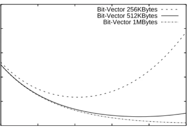
Bit-Vector 256KBytes Bit-Vector 512KBytes Bit-Vector 1MBytes
Figure 7: Error Distribution Variance vs. Quanti-zation Levels
fication outcomev is independent to the token when mis-classifciations occur, and thusvfollowsG(α= 0.5, σ/(2q)). With these assumptions, the lookup errorElookup follows a
Gaussian distributionG(α= 0, σ+σ/(2q)).
In addition, assuming the lookup misclassification occurs independently from the quantization errors, the linear com-bination of two Gaussian distributions is still a Gaussian distribution. The overall query outcome error thus has a meanαof 0, and variance is
(1−Pm,n,h,q)∗(0.5/q) +Pm,n,h,q∗(σ+σ/(2∗q)) (10)
in which, Pm,n,h,q is the misclassification probability of a
Bloom filter that hasqlevels of quantizations,hhash func-tions, total sizembits, and store values forn tokens. The best quantization level isqsuch that it minimizes the value of Equation 10.
Figure 7 shows the predicted error variances of the over-all lookup error distribution assuming σ = 1. The result indicates that for a dictionary of 220,000 tokens, the quan-tization levels should be around 4 to achieve a smaller error variances for small bit-vector size (e.g 256Kbytes). Quan-tization levels smaller than 4 or larger than 6 would have larger error on average. When larger bit-vector is used, quantization levels larger than 4 lead to smaller errors.
Figure 8 shows the predicted error variance for a Bloom filter with the same dictionary size, a fixed quantization level of 4, but with different hash functions. The result matches the intuition that, for a fixed quantization level, the selection of other Bloom filter parameters (h and m) agrees with early studies [4, 5]: for small bit-vector size, the number of hash functions needs to be small (around 6 for the 256Kbytes Bloom filter) in order to achieve a lower misclassification rate. As size of Bloom filter increases, more hash functions can be used to achieve a lower misclassification rate, but the increase in effectiveness is modest.
The above estimation is based on an unrealistic assump-tion of value distribuassump-tions. In real messages, the occurrence of tokens is not independent and identically distributed (iid). This result is only for analytical purpose and is only shown as a guideline for selecting the Bloom filter parameters. The real error rate is determined by the specific distributions and
0 0.2 0.4 0.6 0.8 1 32 16 8 4 2 1
Variances of the Error Distribution
Number of Hash Functions
Dictionary=220,000 Tokens; 4 bits Quantization; Bit-Vector 256KBytes Bit-Vector 512KBytes Bit-Vector 1MBytes
Figure 8: Error Distribution Variance vs. Number of Hash Functions
messages. Furthermore, our overall concern is the final mes-sage classification performance (false positives, false nega-tives, and throughput). Therefore we used real messages to make a realistic study through experiments in order to evaluate the selection of the Bloom filter parameters. The results are presented in Section 4.
3.3.2
Policy for Multi-Bit Errors
The previous subsection discusses the selection of Bloom filter parameters to minimize the possibility of lookup er-rors. Although very rarely, error could still occur. When a conflict caused by multiple bits marking occurs, interpreting the outcome based on any bit could cause lookup error which later could potentially cause a message misclassification.
Although this can not be completely avoided, the impact of this error can be further minimized by making error bi-ased toward a false negative classification rather than a false positive. When multiple possible values come out from one lookup query, we chose the smallest value as the Bloom fil-ter outcome so that even if it is wrongly chosen, the error only makes the classification result less likely as spam. We evaluated the effectiveness of this policy and the result is presented in Section 4.
3.3.3
Selection of Hash Functions
Another fact that can affect Bloom filter lookup speed is the complexity of the hash functions. Popular hash func-tions, such as MD5 [24], have been designed for crypto-graphic purposes. However, the effort to prevent informa-tion leaking is not the focus of hash-based lookup, whose main concern is the throughput. Therefore, simple but fast hash functions are preferred. This strategy of choosing sim-ple hash functions has also been used in [9, 18]. We de-signed a hash function by simplifying the well-known MD5 hash function. Details of the hash function selection are presented in the evaluation section.
4.
EVALUATION
This section presents our experimental evaluation of HAI filters. First we describe our methodology. Second we show the effect of changing Bloom filter parameters.
4.1
Methodology
We studied the effectiveness of HAI filters by measuring its throughput and filter accuracy with real messages (24,000 ham messages and 24,000 spam messages) obtained from the Internet. The ham messages are from the ham training set released by SpamAssassin [27] and from several well-known mailing-lists, including end-to-end [8] and perl monger [22]. The spam messages are obtained from SpamArchive [17]. We split the data set into a training set and a test set. Throughout this section, except explicitly specified, we use 10,000 spam messages and 10,000 ham messages as the train-ing set, which produces a dictionary with 320,976 tokens. The rest of the messages are used for filter testing. The testing sets are further divided to two sets based on their sources. Dataset1 is composed of 10,000 ham from mailing-lists and 10,000 spam from SpamArchive [17]; dataset2 is composed by 4000 ham messages from SpamAssassin [27] and another 4000 spam from SpamArchive.
The experiments are conducted on a PC server with a AMD Athlon64-3000 CPU, 1GB RAM and 512KB Level 2 cache. The CPU speed is scalable by software and by default runs at 1.8GHz. To avoid disk I/O latency, we create ramdisk to store the test set, so that only non-disk I/O are involved for message processing in the experiments.
We built two HAI filters based on well-known Bayesian filters: bogofilter [23] and qsf [30]. Since bogofilter is faster than qsf according to both our measurements and other studies [15], except explicitly specified, all experimental re-sults presented in this section are in the form of a compar-ison between the bogofilter based HAI (labeledHAI filter) versus the original bogofilter (labeled bogofilter) under the same experiment condition.
4.2
Overall Performance
This section summarizes the overall HAI performance with well-selected Bloom filter parameters. The results presented in this section are based on a Bloom filter with a total size of 512 Kbytes, 4 hash functions, and an 8-bit quantization. The performance comparison results are in terms of both filter throughput (messages per second) and filter accuracy (both false positives and false negatives). The filter accu-racy results presented in this subsection are based on a fil-ter threshold of 0.5. Detailed studies for the selection of this threshold as well as other Bloom filter parameters are presented in the later part of the evaluation section.
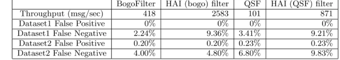
Table 1 shows the overall performance of bogofilter, qsf, and their HAI modifications. This result indicates that, for a Bloom filter size at 512KB, HAI filters can handle 2583 mes-sages per second (i.e. 42Mbps for 2KByte size mesmes-sages). HAI gets a 6 to 8 times throughput speedup compared to bogofilter and qsf respectively, without introducing any ad-ditional false positives. The speedup comes with the penalty of higher false negative rates for HAI filters. Such penalty (e.g. about 7% of overall spam in dataset1) might look sig-nificant, but that still corresponds to more than 90% spam messages being blocked by the filter1. Whether this
trade-off is worthy or not completely depends on each particu-lar site’s needs. The goal of this paper is not to advocate high throughput over accuracy but to provide a study of
1We investigated the nature of those messages that causes
additional false negatives to HAI. Most of them are non-English messages. It just happens to be the case that more of these spam are selected to Dataset1 than Dataset2.
0 500 1000 1500 2000 2500 3000 3500 4000 4500 5000 1.0GHz 1.2GHz 1.4GHz 1.6GHz 1.8GHz
Per Message Time (microseconds)
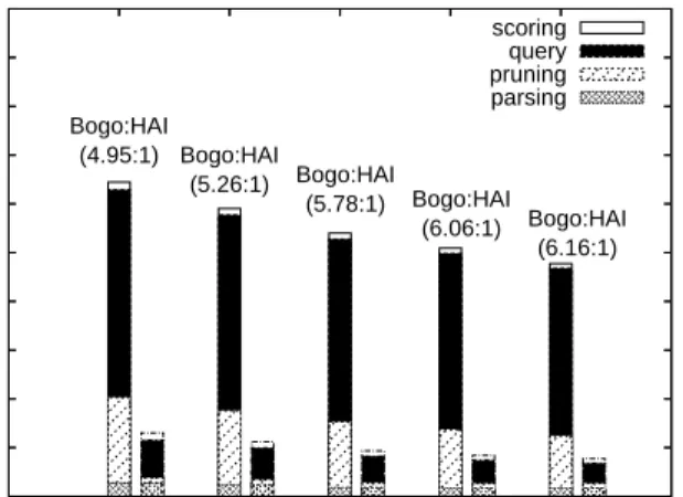
CPU Speed Bogo:HAI (4.95:1) Bogo:HAI (5.26:1) Bogo:HAI (5.78:1) Bogo:HAI (6.06:1) Bogo:HAI (6.16:1) scoring query pruning parsing
Figure 9: Filter Process Time Breakdown for Var-ious CPU Speed (HAI filter: 512KB bit-vector, h=4,q=8; Numbers inside the figure are speedup ratio)
the trade-off between throughput increment and accuracy penalty. Furthermore, multiple levels of spam filtering can be used. For example, HAI filter quickly scanning all in-coming messages, and later applying heavy filters only to “unsure” messages.
4.3
Detailed Breakdown for Throughput
This section presents an in-depth study on the source of this speedup by looking at the detailed behaviors of bo-gofilter and HAI filter. We decompose both bobo-gofilter and HAI to four steps (parsing,pruning,queryandscoring) and measure the time spent on each step per message. Among these 4 steps, the parsing, query and scoring steps have been described in the overview of Bayesian filter in section 2.1. To reiterate, theparsingstep divides the message to tokens based on common delimiters; thequerystep takes each token and uses it as a key for a database lookup to retrieve the cor-responding token statistics; and the scoringstep combines all the query outcomes and calculates an overall message spamminess value.
Bogofilter adds apruningstep betweenparsingandquery. Performance-wise, this pruning step is used to reduce the un-necessary lookup. It removes duplicated tokens so that each unique token only triggers one query. It also eliminates to-kens that are believed to be useless for anti-spam. Such tokens include email message id, MIME labels etc. They are discarded during the training phase and thus are not in the token database (DB). The pruning step of our HAI filter only preserves the function of removing duplicated to-kens to keep the same scoring method (each token counts only once). It uses a standard (not extended) Bloom filter to check token duplications. This Bloom filter works inde-pendently to the extended Bloom filter for the query step. The duplicate token checking initializes a small Bloom filter (2KB in our implementation) to all zeros for each incoming message, and queries and trains the filter at the same time. When a token arrives, it is first tested against the Bloom filter. If the membership testing returns true, the token is considered a duplicate and discarded. Otherwise, the token
Table 1: Performance Comparison between Bogofilter, QSF and HAI Filters on a PC Server with AMD Athlon64 (m=512K, h=4, q=8, thresh=0.5, and CPU=1.8GHz)
BogoFilter HAI (bogo) filter QSF HAI (QSF) filter
Throughput (msg/sec) 418 2583 101 871
Dataset1 False Positive 0% 0% 0% 0%
Dataset1 False Negative 2.24% 9.36% 3.41% 9.21% Dataset2 False Positive 0.20% 0.20% 0.23% 0.23% Dataset2 False Negative 4.00% 4.80% 6.80% 9.83%
is put in the Bloom filter as a new member token and will be used in the query step. The detailed algorithm for this duplication checking can be found in our early work on fast packet classification [5].
We measured the processing time for each step by test-ing bogofilter and HAI with Dataset1. The average message size for Dataset1 is around 2KByte, and each message con-tains about 180 unique tokens. Figure 9 shows the bogofilter versus HAI processing time comparison per message. It is obvious that query and pruning are the two bottleneck steps of bogofilter, and the speedup of HAI comes from these two steps. HAI gains speedup for the query step by reducing the number of memory accesses for each token lookup. An HAI filter’s lookup requires a small amount of memory ac-cesses that only depends on the number of hash functions and the size of Bloom filter, not the total number of stored tokens as in the database lookup case. In addition, by mak-ing the bloom filter size small, most or all of it can fit in cache for lower memory access latency. This effect of cache size is presented in the next subsection. Bogofilter’s query step, on the other hand, operates on Berkeley DB, which is implemented by a Btree. The query requires multiple com-parisons between the input token and tokens in the DB and the number of comparison on average is proportional to the logarithmic of the total tokens in the DB. Although a faster indexing mechanism is possible, a DB lookup essentially has to have a few token comparisons, whereas these comparisons are completely avoided in HAI by the use of the extended Bloom filter.
The HAI also gains significant speedup in its pruning step. We did not include this as part of the general HAI solu-tion for two reasons. First, not all the Bayesian filters avoid searching duplicated tokens as bogofilter does. Second, there is no fundamental reason that a DB-based Bayesian filter can not replace its pruning step with the one used by HAI. Even if bogofilter adopts the same pruning step as HAI, without changing to approximate query as HAI does, bo-gofilter would still be multiple times slower than HAI to process a message.
In addition to the throughput gain against bogofilter, HAI’s throughput scales better as CPU speed increases. The AMD Athlon64 based desktop supports CPU scaling, we adjusted the speed from 1.0 GHz to 1.8GHz and measure the through-put of both filters. Figure 9 shows a comparison of bogofilter and HAI for various CPU speeds. Although both filters take less time to process a message as the CPU speed increases, the speedup ratio for HAI versus bogofilter increases as CPU speed becomes higher.
We also inspect the effect of message size on the speedup ratio. As messages get large, the speed up ratios are about the same but with a slight decrease. The parsing step in-creases strictly proportional to the message sizes, but the
Table 2: AMD L2 Cache Performance Counters for the Query Step Per Message (CPU=1.8GHz, and for HAI filter: h=4, q=8)
Configuration L2 Miss L2 Hit Query Time HAI (128KB) 8 835 202µs HAI (256KB) 30 1120 208µs HAI (512KB) 51 1264 216µs HAI (1MB) 387 1066 257µs BogoFilter 2157 605 1716µs
number of unique tokens does not increase in a strict linear fashion. The bottleneck starts to shift from query and prun-ing toward parsprun-ing. However, even with a jumbo message size, token query continues consuming a significant amount of processing time for bogofilter, and approximate classifi-cations would still improve bogofilter’s performance.
4.4
Effect of Bloom Filter Size
In this subsection we study the effect of Bloom filter size on the filter accuracy and processing throughput. Both the throughput and accuracy measurements were obtained from experiments using the Dataset1.
For the effect of Bloom filter size on throughput, Figure 10 shows that the per message processing times are about the same for the HAI filters with a Bloom filter size less than 512KB. After the bloom filter becomes close to or exceeds L2 cache size (512KB), the processing time in general increases as the Bloom filter size increases towards 16 Megabytes. The AMD Athlon64 processor provides performance coun-ters for specific processor events, such as data cache hits and misses, to support memory system performance monitoring. To confirm the cache size effect, we capture the L2 cache performance counters before and after each query step.
Table 2 contains the average L2 memory access and miss counters of the query step for HAI or bogofilter to process a message. As shown by Table 2, smaller Bloom filters can be put in higher level CPU caches and have fewer cache misses compared to larger Bloom filters. HAI filters clearly have a higher L2 hit rate than bogofilter. L2 cache behavior is not the single factor that determines the processing time; the total computation of a program, memory access pat-tern, as well as L1 cache behaviors all affect the query time, and a slight adjustment to the program (e.g different Bloom filter sizes) could change these memory accesses behaviors. This is also why the total L2 accesses (hits+misses) changes across different filter setups. Although we can not directly calculate the query time from L2 misses, it is clearly that the cache accesses differences is a major source for the query time increment over filter size increment, which is shown in Figure 10.
0 20 40 60 80 100 0 0.2 0.4 0.6 0.8 1
False Positive (Percentage)
Threshold Bogofilter 64k 128k 256k 512k 16M 0 20 40 60 80 100 0 0.2 0.4 0.6 0.8 1
False Negative (Percentage)
Threshold Bogofilter 64k 128k 256k 512k 16M
Figure 11: Filter Accuracy vs. Bloom Sizes (h=4, q=8). Results with 1MB to 8MB bit-vectors are all between the results of 512KB and 16MB and thus not shown in the Figure
0 50 100 150 200 250 300 350 400 450 500 16M 8M 4M 2M 1M 512K 256K 128K 64K
Per Message Time (microseconds)
Bloom Fitler Size (Bytes) scoring
query pruning parsing
Figure 10: Processing Time VS. Bloom Sizes (CPU=1.8GHz,h=4,q=8)
The gain in throughput comes with a penalty on filter ac-curacy. To have an overall picture about how much change was brought to the filter accuracy by HAI, we present the false positive and false negative probabilities for the com-plete range of possible filtering thresholds from 0 to 1. Fig-ure 11 shows a summary of the filter accuracy for HAI filters with various Bloom filter sizes ranging from 64KB to 16MB. For the false positive result shown on the left half of Figure 11, HAI filters with smaller than 512KB show significant differences compared to those of bogofilter. The smaller the Bloom filter size, the higher differences they can make.
However, for Bloom filter sizes larger or equal to 512KB, the email scores for ham messages are in fact very close to 0 and thus the false positive rates stay low. All filters have a close to zero false positive after the threshold gets larger than 0.5, even for those with a small Bloom filter size. This effect is due to the way that email score is calculated by Equation 2, which tends to produce a value around 0.5 to a randomly generated message. When token
misclassifica-tion occurs, the lookup outcome is close to the outcome of a randomly generated message. Therefore, higher token mis-classification rates tend to push an email (ham or spam) score toward 0.5, and both the false positives and false neg-atives results exhibit a significant change at threshold 0.5, no matter what Bloom filter sizes are used.
The false negative rate, which is measured over spam mes-sages, is shown at the right half of Figure 11. The false neg-ative result is similar to the false positive result in the sense that larger Bloom filter size gives closer results to the orig-inal bogofilter, and filters smaller than 512KB differ from bogofilter more significantly than those with a larger than 512KB bit-vector. Furthermore, compared to false positive, the results of false negatives show a relatively larger gap between the bogofilter outcome and HAI filter, even with a large bit-vector at 16MB. We believe this is due to the quantization errors. A closer look at various quantization levels is presented later in this section. The accuracy results for HAI certainly also depends on the test data set as well as the training data set. Our experiences of HAI filter with other datasets also showed a similar accuracy-throughput tradeoff.
4.5
Effect of Hash Functions
We consider two aspects of hash functions, the hash com-plexity and the number of hash functions, for the HAI filter performance. We compare two hash functions: MD5 and MD-. MD5 is picked to represent the well-known crypto-graphic hash functions that provide a well distributed hash output. MD- is our modification of MD5 to represent a sim-pler but faster hash. The core of MD5 is a combination of 4 “bitwise parallel” functions named F, G, H, and I by the specification [24]. MD- only uses the F function but with the same initial and end bit shuffles as in MD5. The re-sults of filter throughput and accuracy measurements are omitted from this paper due to space limitations. Overall, our results show that the throughput of MD- based filter achieves about 10% higher throughput than the MD5 based filters. For accuracy measurement, the false positive rates are close to identical for MD- and MD5. The false negative results are also very close to each other. This similar result
0 20 40 60 80 100 32 16 8 4 2
False Negative (Percentage)
Number of Hash
Bogofilter HAI
Figure 12: Filter Accuracy vs. Number of Hash Functions (m=512KB, q=8 bit, thresh=0.6)
on accuracy indicates that simple and fast hash functions are the better choice for Bloom filter based approximations. We are currently working on a further simplified hash func-tion to achieve higher throughput while preserving similar accuracy.
We also investigated the effect of using a different number of hash functions. Using a small number of hash functions reduces the number of marked bits, but has a higher prob-ability of hash conflicts. Meanwhile using a large number of hash functions causes too many bits set in a Bloom fil-ter with a limited bit-vector size and affects the accuracy. Figure 12 shows the filter accuracy results when using differ-ent numbers of hash functions. The bogofilter false negative result is also shown in the figure as a reference. Only the false negative result is shown here because the false positive results are all zero. For the size of 512K byte Bloom fil-ter, Figure 12 demonstrates that the best choice is to use 8 hashes, with both 4 and 16 hashes having very close results.
4.6
Effect of Quantization Levels
This section presents the experimental results on the effect of quantization level selection. The results were obtained in two steps. First, we isolated the effect of quantization from Bloom filter misclassifications. To study the quantization effect alone, we applied it directly to bogofilter by quantizing all its statistical data in the database, and then measured its accuracy. Second, we did experiments with HAI filters with different quantizations levels.
Figure 13 compares the filter accuracy among three cases: the original bogofilter, bogofilter with quantizations, and HAI filters, with the number of quantization bits set from 2 to 16. Quantization introduces errors to data representa-tion, which in general reduces filter accuracy. The original bogofilter’s accuracy result is used as the best-case reference to compare the performance of filters with various quantiza-tion levels. As expected, for bogofilters with quantizaquantiza-tion, 16 bits quantization performs best, but a quantization level around 4 to 8 is also close to the original non-quantized case. However, for HAI filters, higher quantization levels no longer produce the closest accuracy results to bogofilter. Instead, a quantization level at 8 shows the best accuracy
0 20 40 60 80 100 16 8 4 2
False Negative (Percentage)
Quantization Level
Bogofilter (with Quantization) Bogofilter HAI
Figure 13: Filter Accurary vs. Quantization Levels (m=512KB, h=4, thresh=0.6)
results. By inspecting the token misclassification rate (by comparing each token outcome to bogofilter outcome), we found that the token misclassification rate increases as more quantizing bits are used. The best quantization level has to be one that balances the quantization error and the mis-classification rate. For the given experiment setup, the best quantization level is 8. Similar to the effect of Bloom fil-ter size, the optimal selection depends on the number of tokens to be stored. Nevertheless, an important outcome from these experiments is that we have shown a small quan-tization level can effectively produce a filter accuracy that is very close to the accuracy of the original bogofilter.
4.7
Strategy for Handling Multi-bit Markings
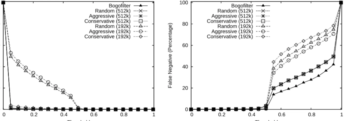
In this section, we consider the strategies for handling the multi-bit marking error that is unique to the value re-trieving extension of Bloom filter. When multi-bit marking occurs, the Bloom filter has to make a decision on the final lookup outcome. We consider three strategies for choos-ing the value. 1) Aggressive Strategy: every time multi-bit marking occurs, we always choose a value which indicates the highest spamminess; 2) Randomly Selecting Strategy: randomly pick one value; 3) Conservative Strategy: we al-ways choose a value which indicates lowest spamminess. Fig-ure 14 shows the effect of different strategies on two Bloom filter sizes, 192KB and 512KB, respectively.
Figure 14 shows the effect of these three strategies for HAI under two different sizes: 192KB and 512KB. The two sizes are chosen to illustrate the impact of strategies under high and low multi-bit marking errors. Equation 8 indicates that the probability for multi-bit marking error is high when the Bloom filter size is small. When Bloom filter size is small (here 192KB) the aggressive strategy always has lower false negative rate than the other two. Meanwhile false positive should follow the reverse trend of the false negative. The aggressive strategy results show a very different false posi-tive measurement compared to bogofilter for any threshold less than 0.5. The conservative strategy gives the best result in the false positive measurement and has about the same false positive as bogofilter. The random selection strategy is somewhere between but much closer to the aggressive
0 20 40 60 80 100 0 0.2 0.4 0.6 0.8 1
False Positive (Percentage)
Threshold Bogofilter Random (512k) Aggressive (512k) Conservative (512k) Random (192k) Aggressive (192k) Conservative (192k) 0 20 40 60 80 100 0 0.2 0.4 0.6 0.8 1
False Negative (Percentage)
Threshold Bogofilter Random (512k) Aggressive (512k) Conservative (512k) Random (192k) Aggressive (192k) Conservative (192k)
Figure 14: Filter Accuracy vs. Value Selection Strategies for Multi-bit Marking (m=512KB, h=4, q=8)
proach. But for larger bit-vectors (here 512KB), the dif-ferences among strategies are small. This is because the overall multi-bit marking error is small. All three strategies lead to very low false positives. Users can retain conserva-tive strategy but still preserve a high filter accuracy. Overall this result indicates that the multi-bit handling strategies do not affect the filter accuracy in a significant way for large bit-vectors. However, to avoid false positives, we still rec-ommend and use the third strategy in all other experiments.
5.
RELATED WORK
Message classification is a well-studied topic with appli-cations in many domains. This section makes a brief de-scription of the related work in two categories: classifica-tion techniques for anti-spam purpose, and fast classificaclassifica-tion techniques using Bloom filters.
5.1
Anti-SPAM Techniques
Anti-spam is a very active area of research, and various forms of filters, such as white-lists, black-lists [6, 16], and content-based lists [13] are widely used to defend against spam. White-list based filters only accept emails from known addresses. Black-list filters block emails from addresses that are known to send out spam. Content-based filters make estimations of spam likelihood based on the text of that email message and filter messages based on a pre-selected threshold. Most of content-based filters use a Bayesian algo-rithm [13] to estimate message spamminess, and have been used in many spam filter products [15]. Recently, there have been several proposals about coordinated real-time spam blocking, such as the Distributed Checksum Clearinghouse [26]. Most of these spam filters focus on improving the spam filter-ing accuracy. The work presented in this paper differs from them by investigating the trade off between accuracy and throughput. We have shown that with a carefully chosen algorithm, Bayesian filters can gain throughput with only a small loss on false negative probabilities.
Many assumptions used by Bayesian filters to combine in-dividual token probability for an overall score, such indepen-dent tokens, are not true for email messages, and more so-phisticated classification techniques, such as k-nearest neigh-bors are proposed. In practice, naive Bayesian classifiers
of-ten perform well [21, 23, 27, 30], and the current state of spam filtering indicates that they work very well for email classifications. Nevertheless, the work presented in this pa-per is to speedup the probability lookup stage for the prob-ability calculation, and we expect the approach is applicable toward more sophisticated classification techniques.
5.2
Fast IP Processing by Bloom Filters
Hash-based compressed data structure has recently been applied in several network applications, including IP trace-back [28], traffic measurements [10] and fast IP packet clas-sifications [5]. For traffic measurement and traceback ap-plications, Bloom filters are used to collect packet statistics and very often using hardware-based Bloom filters [7]. The work presented in this paper uses Bloom filters to improve software processing speed, and investigate the trade off be-tween throughput and accuracy. Among all these previous Bloom filter applications, the closest related work is the high speed packet classification using Bloom filters, which first studied the tradeoff between accuracy and the processing speed. This previous study uses Bloom filters for member-ship testing, the work in this paper uses an extended Bloom filter that supports value retrieving. In addition, we consid-ered an additional level of approximation by applying lossy encoding to data representations.
6.
CONCLUSIONS
In this paper, we have explored the benefit of using ap-proximate classification to speed up spam filter processing. Using an extended Bloom filter to make approximate lookup and lossy encoding to approximately represent the statistic training data, we demonstrate a significant speedup over two well-known spam filters (bogofilter and qsf). The result also shows that with careful selection of Bloom filter param-eters, the errors introduced by the approximation becomes very small and the high speed filter with approximation can achieve very similar false positive and false negative rate as normal Bayesian filters. Currently we are working on apply-ing the same technique to other Bayesian spam filters and designing techniques to improve other types of anti-spam systems.
7.
ACKNOWLEDGMENTS
We wish to thank the following people for their contribu-tions to the system or the paper. We would like to thank Dan Rubenstein for his excellent shepherding. We also thank the anonymous reviewers for their many helpful suggestions. Thanks to Barry Rountree for his help with AMD perfor-mance counters and comments on this paper. This work is sponsored by a Georgia Research Alliance grant GRATC06G.
8.
REFERENCES
[1] I. Androutsopoulos, J. Koutsias, K. Chandrinos, G. Paliouras, and C. Spyropoulos. An evaluation of naive bayesian anti-spam filtering. InProceedings of the workshop on Machine Learning in the New Information Age, 2000., pages 9–17, May 2000. [2] T. Berger and J. D. Gibson. Lossy source coding.
IEEE Transactions on Information Theory, vol.44(6):2693–2723, 1998.
[3] B. Bloom. Space/time trade-offs in hash coding with allowable errors.Communications of the ACM, vol.13(7), July 1970.
[4] A. Broder and M. Mitzenmacher. A survey of network applications of bloom filters.Internet Mathmatics, vol.1(4):485–509, 2004.
[5] F. Chang, K. Li, and W. Feng. Approximate packet classification caching. InProceedings of IEEE Infocom 2004, March 2004.
[6] M. Delio. Not all asian email is spam. InWired News Article, Feb 2002.http://www.wired.com/news/ politics/0,1283,50455,00.htmlLast accessed Feb 26, 2006.
[7] S. Dharmapurikar, P. Krishnamurthy, and D. E. Taylor. Longest prefix matching using bloom filters. In
in Proceedings of ACM SIGCOMM 2003, pages 201–212, August 2003.
[8] End-to-End Interest Research Group. The end2end-interest archives.http:
//www.postel.org/pipermail/end2end-interest/
Last accessed Feb 27, 2006.
[9] O. Erdogan and P. Cao. Hash-av: fast virus signature scanning by cache-resident filters. Inin Proceedings of Globecom’05, November 2005.
[10] C. Estan and G. Varghese. New directions in traffic measurement and accounting. InProceedings of Internet Measurement Workshop, pages 75–80, November 2001.
[11] L. Fan, P. Cao, J. Almeida, and A.Z.Broder. Summary cache: a scalable wide-area web cache sharing protocol.IEEE and ACM Transaction on Networking, 8(3):281–293, 2000.
[12] D. Gall. MPEG: A video compression standard for multimedia applications. InCommunication of ACM, pages 46–58, April 1991.
[13] P. Graham. A plan for spam, Janurary 2003. In the First SPAM Conferencehttp://spamconference.org.
[14] D. Heckerman and M. P. Wellman. Bayesian networks. InCommunications of the ACM, number 3, pages 27–30, March 1995.
[15] S. Holden. Spam filter evaluations.
http://sam.holden.id.au/writings/spam2/ Last accessed Nov 2, 2005.
[16] P. Jacob. The spam problem: moving beyond RBLs, 2003.http://theory.whirlycott.com/~phil/ antispam/rbl-bad/rbl-bad.html Last accessed Feb 26, 2006.
[17] P. Judge. The SPAM archive.
http://www.spamarchive.org Last accessed Feb 26, 2006.
[18] K. Li, F. Chang, W. chang Feng, and D. Burger. Architecture for packet classification caching. In
Proceedings of IEEE ICON’2003, May 2003. [19] D. Lowd and C. Meek. Good word attacks on
statistical spam filters. InProceedings of the Second Email and SPAM conference, July 2005.
[20] J. Max. Quantizing for minimum distortion.IEEE Transactions on Information Theory, vol.28(2):7–12, 1960.
[21] T. Meyer and B. Whateley. SpamBayes: Effective open-source, bayesian based, email classifications. In
Proceedings of the First Email and SPAM conference, July 2004.
[22] Perl Monger Users. Perl monger mailing-list.
http://mail.pm.org/pipermail/classiccity-pm/
Last accessed Feb 27, 2006.
[23] E. S. Raymond. Bogofilter: A fast open source bayesian spam filters.
http://bogofilter.sourceforge.net/ Last accessed Nov 2, 2005.
[24] R. Rivest. The MD5 message-digest algorithm.RFC 1321, April 1992.
[25] G. Robinson. A statistical approach to the spam problem. In Linux Journal 107, March 2003, http: //www.linuxjournal.com/article.php?sid=6467
Last accessed Nov 2, 2005.
[26] V. Schryver. Distributed spam clearinghouse.
http://www.rhyolite.com/anti-spam/dcc/ Last accessed Nov 2, 2005.
[27] M. Sergeant. Internet level spam detection and spamassassin. InProceedings of the 2003 Spam Conference, January 2003.
[28] A. Snoeren, C. Partridge, L. Sanchez, C. Jones, F. Tchakountio, S. Kent, and W. Strayer. Hash-based IP Traceback. InProceedings of ACM SIGCOMM’01, August 2001.
[29] G. L. Wittel and S. F. Wu. On attacking statistical spam filters. InProceedings of the First Email and SPAM conference, July 2004.
[30] A. Wood. Quick spam filter.
http://freshmeat.net/projects/qsf/ Last accessed Nov 2, 2005.