the Earned Income Tax Credit. Review of Economics of the Household.
ISSN 1573-7152 , http://dx.doi.org/10.1007/s11150-018-9429-x
This version is available at https://strathprints.strath.ac.uk/64942/
Strathprints is designed to allow users to access the research output of the University of Strathclyde. Unless otherwise explicitly stated on the manuscript, Copyright © and Moral Rights for the papers on this site are retained by the individual authors and/or other copyright owners. Please check the manuscript for details of any other licences that may have been applied. You may not engage in further distribution of the material for any profitmaking activities or any
commercial gain. You may freely distribute both the url (https://strathprints.strath.ac.uk/) and the
content of this paper for research or private study, educational, or not-for-profit purposes without prior permission or charge.
Any correspondence concerning this service should be sent to the Strathprints administrator:
strathprints@strath.ac.uk
The Strathprints institutional repository (https://strathprints.strath.ac.uk) is a digital archive of University of Strathclyde research outputs. It has been developed to disseminate open access research outputs, expose data about those outputs, and enable the
https://doi.org/10.1007/s11150-018-9429-x
The effects of income on health: new evidence from
the Earned Income Tax Credit
Otto Lenhart 1
Received: 9 February 2018 / Accepted: 28 July 2018 © The Author(s) 2018
Abstract
This study examines the relationship between income and health by using an expansion of the Earned Income Tax Credit (EITC), which increased benefits to households with at least two children, as a source of exogenous variations of earnings. The paper adds to previous work by: (1) estimating treatment effects on the treated using simulated EITC benefits and longitudinal data; (2) testing whether health effects vary across the three different parts of the EITC schedule; (3) examining the role of food expenditures and health insurance as potential mechanisms. The studyfinds that income improves the likelihood of affected heads of households reporting to be in excellent or very good health by 6.9 to 8.9 percentage points. The effects are largest in the plateau phase of the EITC schedule, where previous researchers have identified pure income effects of the program. The results are robust to several additional specifications, including a semi-parametric DD model and specifications that account for the potential endogeneity of sample. When examining potential channels underlying the relationship between income and health, Ifind that affected household increase their food expenditures by 10.5 to 20.3 percent and are 1.52 percent more likely to have health insurance coverage.
Keywords Income ●Health●Earned Income Tax Credit●Food expenditures JEL classifications I14●I38●J38
* Otto Lenhart
ottolenhart@gmail.com
1 University of Strathclyde, Department of Economics, Duncan Wing, Strathclyde Business School 199
Cathedral Street, Glasgow, UK
Electronic supplementary materialThe online version of this article ( https://doi.org/10.1007/s11150-018-9429-x) contains supplementary material, which is available to authorized users.
123456789
1 Introduction
The existence of a significant positive association between income and health, also known as the income gradient in health, has been well documented in the literature (Case et al.2002; Deaton2002). Despite several contributions over the past decade in a number offields, which have found robust correlations using data from different countries, it is still not entirely clear whether such a positive association is the result of a causal relationship between income and health. There are good reasons to believe that a causal effect between income and health exists. Higher income families may have better access to care as well as more opportunities to purchase care; whereas people with lower income may be confronted with more stressful situations, which are detrimental to health. This study tests whether the well-established health gradient exists once the endogeneity of income is accounted for by using expansions in the Earned Income Tax Credit (EITC) in the mid-1990s as a source of exogenous income variation. Ifind that higher EITC payments lead to significant improvements in self-assessed health, while changes in food expenditures and insurance coverage are shown to be likely mechanisms underlying the relationship between income and health.
By using data from the Panel Data of Income Dynamics (PSID) for the years 1990–2003, this study exploits the expansion of the EITC, which was part of OBRA 1993, to test for the relationship between income and health outcomes of heads of households. This approach can eliminate or significantly reduce the omitted variable bias due to shocks correlated with income and give estimates for treatment effects of receiving a boost in income on health of treated individuals. Findings for the rela-tionship between income and health in this setting add to previous work on the gradient and provide evidence for a causal effect of income on health. Additionally, the later part of the study tests for the role of food expenditures and health insurance as potential mechanisms underlying the link between income and health.
Several recent studies on the EITC have examine whether the program is able to improve health outcomes of children (Baughman and Duchovny2016; Averett and Wang 2016), infants (Hoynes et al. 2015), mothers (Evans and Garthwaite 2014), and low-income adults (Larrimore2011). This study joins this small group of papers and adds to them by makingfive contributions. First, the use of a longitudinal data set and individual fixed effects models can improve the identification strategy by accounting for time-invariant unobserved heterogeneity, potential changes in the sample composition, and measurement error in self-assessed health. Since it is possible that there are systematic differences between families with one child and two or more children that change over time, accounting for individual un-observables can reduce the potential bias of the results. Given that the EITC provides incentives for low-income individuals to enter the labor force, the use of longitudinal data helps account for differences in the composition of sample before and after an expansion of the program. Additionally, potential measurement errors can be reduced since each individual’s health is only compared to their own prior assessment, which takes into account that respondents might have their own scales in ranking their health (reference bias). To my knowledge, only one previous paper uses longitudinal data to analyze the relationship between the EITC and health (Averett and Wang2016).
Second, I use a tax simulator program to obtain predicted EITC payments and to examine health changes among a sample of individuals eligible to receive EITC benefits. Previous studies testing for health effects of the EITC have focused on low-educated individuals, a group most likely affected by changes to the program. Examining health changes among low-educated samples provides intent-to-treat estimates for the effects of the policy change. Given that take-up rates for the EITC have been shown to be between, 80 and 87% (IRS2002; Scholz1994), I believe that my analysis is able to provide estimates that are closer to treatment effects on the treated. These can provide evidence for whether income in general has causal effects on health. It should be noted that my study assumes full take-up rates of the EITC and therefore the estimated effects will underestimate the true effects on treated individuals. Overall, thefindings from this study complement the great work pre-viously conducted on the relationship between the EITC and health, while specifi -cally addressing the relationship between income and health.
Third, the study uses the imputed simulated EITC amounts which respondents are eligible to receive in order to further examine the link between income and health in more detail. Specifically, I test whether the expansion had different health impacts for individuals falling in different parts of the EITC schedule (phase-in, plateau, and phase-out range). Previous work has established that individuals in the plateau part receive close to pure income effect (Athreya et al.2010; Gunter2013), while those in the phase-in part have been found to work more on the extensive margin (Eissa and Liebman1996; Eissa et al. 2008; Meyer 2010). Thus, testing for different health effects across the three parts of the schedule can provide evidence whether cash transfer programs have different effects depending on if they are conditional on earned income. Additionally, I test whether health effects differ for individuals who experienced relatively large increases in EITC compared to those who experienced smaller increases, which can provide additional evidence for the effects of income on health.
Fourth, this study contributes to the remaining uncertainty regarding the mechanisms through which income can affect health outcomes by investigating the role of two potential channels. To my knowledge, this is thefirst study that examines the role of changes in food expenditures as a potential channel through which higher EITC benefits might affect health. Given that there is a close link between income and food insecurity, additional income in the hands of vulnerable groups of the population could affect their levels of food security. Furthermore, similar to work by Baughman (2005) and Hoynes et al. (2015), this study tests for the role of changes in health insurance coverage following an expansion of the EITC.
Fifth, besides estimating DD models, I test for the robustness of thefindings by additionally estimating several other specifications. These include: (1) a DDD model that accounts for the fact that other events at the time could impact health outcomes of individuals in the sample; (2) a semi-parametric DD model which loosens some assumptions about a linear relationship between income and health; (3) a model that only includes individuals who are eligible to receive EITC benefits prior to the policy change; (4) a model that includes all individual below certain income thresholds, irrespective of eligibility; (5) a falsification test that compares health changes of two groups that were equally affected by the expansion, (6) three different specifications that test for the presence of reverse causality.
This study finds that increases in income following the expansion of the EITC leads to improvements in self-reported health status among heads of household affected by the policy change. Affected individuals are 6.9 to 8.9 percentage points more likely to report excellent or very good health status following the policy change. The positive health effects are robust to variations in both sample selection and methodology and become larger when the policy change is allowed to have a 1-year adjustment period after its implementation. The analysis shows that health benefits were largest for people in the plateau phase of the EITC, which provides further evidence that the health improvements are the result of increases in income. When examining potential mechanisms underlying the link between income and health, this paper provides evidence that increases in food expenditures and take-up rates of insurance can explain the observed health improvements. Specifically, Ifind that affected household increase their food expenditures by 10.5 to 20.3% and are 1.52% more likely to have health insurance coverage
2 Previous literature
A number of previous studies have investigated the relationship between household income and self-reported health status. Case et al. (2002) set the groundwork for this area of research byfinding a significant positive relationship between family income and health of children younger than seventeen years of age in the United States. Applying similar setups as Case et al. (2002), many studies have since then inves-tigated the existence of an income/health gradient in Canada (Currie and Stabile
2003), England (Currie et al. 2007; Propper et al. 2007), Australia (Khanam et al.
2009), and Germany (Reinhold and Jürges2012). Based on the convincing evidence of thefindings in these studies, the existence of the income gradient in health became established and widely acknowledged.
The observed positive association between income and health, however, does not necessarily reflect a causal link from income to health due to the potential endo-geneity of income. There might be third factors, such as living environment and access to better health care, education, stress or genetics, which might explain why some individuals are better offfinancially and in better health than others are. Smith (2007) provides evidence that health outcomes are influenced by education and not by financial resources. Another source of endogeneity is the potential for reverse causality, which occurs if changes in health outcomes affect people’s income. Smith (1999, 2005) shows that health determines household income and wealth for indi-viduals nearing retirement, while Case and Paxson (2011) use data from the Whitehall II Study to show that health and socioeconomic status during childhood impact people’s success in the workforce when they are adults.
A number of studies have so far addressed whether the established positive association between income and health reflect a causal relationship by estimating instrumental variable models to account for the potential endogeneity of income. The following instruments for income and wealth have been used by researchers in the past: parental education, work experience, spousal characteristics (Ettner 1996),
inheritances (Meer et al.2003; Economou and Theodossiou2011), lottery winnings (Lindahl 2005; Gardner and Oswald 2007; Apouey and Clark 2015), income transfers from to individuals in East Germany following German Reunification (Frijters et al.2005), and local unemployment rates (Ettner 1996; Kuehnle 2014). Adda et al. (2009) exploit changes in macroeconomic conditions at the cohort level and model income and health as a stochastic process, which evolves over the life cycle. Overall, the evidence provided by these studies is very mixed, resulting in the fact that there is still some uncertainty about the causal nature of the relationship. While somefind no evidence that income leads to improved physical health (Meer et al.2003; Lindahl2005; Adda et al.2009; Apouey and Clark2015), others provide evidence for a potential causal link (Ettner1996; Frijters et al.2005; Kuehnle2014; Economou and Theodossiou 2011). Furthermore, two studies suggest that income might cause improved mental health outcomes (Gardner and Oswald2007; Apouey and Clark2015). A potential explanation for the mixed findings are concerns about the exogeneity of some of the variables used.
The majority of previous work on the EITC has focused on the effects on eco-nomic outcomes. The existing literature has established that changes in the EITC are a successful tool in lifting families above the poverty threshold (Scholz 1994; Neumark and Wascher 2001; Meyer 2010; Short 2014; Hoynes and Patel 2015). Based on the U.S. Census Supplemental Poverty Measure, in 2013 the EITC (and the child tax credit) lifted 4.7 million children out of poverty, which is more than any other program (Short 2014). Hoynes and Patel (2015) show that a policy-induced $1000 increase in the EITC leads a 9.4 percentage point reduction in the share of families with after-tax and transfer income below 100% poverty. Furthermore, researchers have investigated the impacts of the program on labor force participation (Eissa and Liebman 1996; Meyer and Rosenbaum 2001; Hotz and Scholz 2003; Eissa et al.2008; McKeehan2017), educational attainment (Miller and Zhang2009), test scores (Dahl and Lochner2012), marriage (Ellwood2000; Dickert-Conlin and Houser2002; Michelmore2018), fertility (Duchovny2001; Baughman and Dickert-Conlin 2009, Meckel 2015), and foster care (Biehl and Hill 2017). Dowd and Horowitz (2011) show that the EITC is often only a short-term safety nets for low-income households by providing evidence that 61 percent of recipients only claim the EITC for one or two years.
Not until very recently have researchers started examining potential effects of the program on health outcomes. Examining expansions of the federal EITC, several studies have found that the EITC is associated with changes in health. The study that is most similar to this one is by Evans and Garthwaite (2014) whofind that the 1993 expansions of the EITC led to improved self-reported health and reduced number of poor mental health days for mothers with two children. Additionally, the authors use data on biomarkers to provide evidence that reductions in stress levels can potentially explain these observed improved health improvements. The results by Evans and Garthwaite are in contrast to those found by Larrimore (2011), which suggest that increases in income following EITC expansions do not improve self-reported health of working age individuals. Hoynes et al. (2015) provide evidence that the EITC reduces the likelihood of low birth weight, while changes in prenatal care, smoking and shifts from public to private insurance are shown to be potential mechanisms
explaining how the program affects birth weight. Averett and Wang (2016)find that higher EITCs can improve mother-rated health for children of married white mothers and unmarried Black and Hispanic mothers. One health outcome that has so far been shown to be negatively affected by higher EITCs is obesity. Two studies provide evidence that expansions of the EITC lead to increases in the likelihood of being obese for both women (Schmeiser2009) and children (Jo2018).
Several recent studies have expanded the research examining health effects of the EITC by examining the effects of state-level variations of the program. Baughman and Duchovny (2016) show that state-level EITCs are associated with significant improvements in health status for children between the ages 6 to 14 as well as with increases in private insurance coverage. Strully et al. (2010) and Markowitz et al. (2017) additionally show that state-level EITCs can improve birth outcomes. Four studies that have focused on outcomes related to health have shown that the EITC increases employer-sponsored health insurance coverage (Baughman2005), reduces smoking of mothers (Averett and Wang2013), and improves both child development (Hamad and Rehkopf2016) and subjective well-being of mothers (Boyd-Swan et al.
2016).
3 Background
3.1 The Earned Income Tax Credit
The Earned Income Tax Credit (EITC) provides a refundable transfer to lower-income working families through the tax system. First enacted in 1975 as a relatively small credit capped at $400 per family to offset the growth of payroll tax payments by families with children, the program was supposed to act as a work bonus as well as a response to the 1974 recession. The EITC was introduced in an attempt to reward work rather than to provide guaranteed income, while aiming at moving families beyond the poverty line. Since the original implementation, Congress has expanded the EITC several times both in terms of benefit size and eligibility requirements. Between 1984 and the early 2000s, the phase-in rate of the EITC increased from 10 to 40% of earnings. OBRA 1993, signed by President Clinton, delivered one of the most significant changes to the tax credit. The reform sig-nificantly increased differences in benefits given to eligible families with two or more children younger than nineteen years of age in the household and those with only one child. As soon as the changes of the reform were fully put in place in 1996, max-imum benefits for families with two or more children more than doubled, whereas payments for families with one eligible child only slightly increased.
Today, the EITC has become the largest cash transfer program as well as the most important anti-poverty policy in the United States. In 2010, over 26 million families received the credit, totaling $58.6 billion in foregone revenue. In comparison, federal expenditures on Temporary Assistance to Needy Families (TANF), previously the largest cash transfer program in the United States, amounted to only $15.2 billion (Office of Family Assistance,2011). In addition to the federal EITC program, many
states have introduced state credits that further enhance benefits given to lower-income working families.1
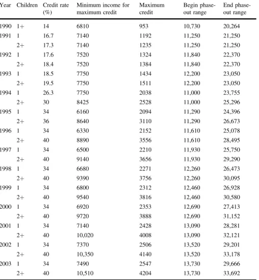
In addition to the augmented importance of the program over the last decades, another reason for why the EITC has attracted much interest by researchers is its unique payment structure, which significantly differs from other welfare programs. The size of benefits received by eligible families depends on several factors, such as the presence and number of qualifying children in the household.2Depending on the amount of a family’s earnings and adjusted gross income, EITC payments have: (1) A phase-in range in which higher earnings yield higher credits; (2) A plateau phase in which payments remain the same even as earnings rises; and (3) A phase-out range in which higher earnings yield lower credits. Following several expansions to the program, the plateau phase expanded from $5000–6000 in 1984 to around $10,000–13,000 in 2003. In 2003, families with household incomes of around $29,000 (one child) and $36,000 (two or more children) are eligible to receive the EITC benefits. Table1 provides an overview of the EITC parameters for families with one and two or more children during the time period of the study. The statistics show that the policy change in the mid-1990s substantially altered the credit rates and benefits to eligible families. While the difference in maximum benefits between families with one child and families with two or more children was $43 in 1991, the difference increased to $1404 in 1996.
An earlier expansion of the EITC through OBRA 1990 introduced the Health Insurance Tax Credit (HITC), which was designed as a supplemental credit for health insurance purchases in order to increase the coverage of low-earning workers. After being in place for only three years, the HITC, which provided credits of up to $465 (Cebi and Woodbury2009), was effectively repealed on 31 December 1993. While the eligibility requirements were similar for EITC and HITC, take up rates differed significantly for the two benefits. Only 19–26% of eligible households received the HITC (U.S. Government Accountability Office 1994), while take-up rates for the EITC were between 80 and 87% (IRS2002; Scholz 1994).
3.2 The EITC and health
The EITC can affect health outcomes through several channels. First, the tax credit can affect health by providing increases in income for individuals from low socio-economic backgrounds. As shown in more detail in Section 4 of the paper, average annual EITC benefits for households benefiting from the expansion were sub-stantially higher after the policy change and exceeded $2000. Meyer (2010) esti-mated the 2007 federal EITC benefits reduced the poverty rate by 10% and lifted over 1.1 million families above the poverty line. Literature on the EITC has estab-lished that the program successfully increases earnings and lifts individuals above the poverty threshold by encouraging work, especially among single mothers (Eissa and 1 Before the policy changes of OBRA 1993 were implemented, seven states had introduced state-level
EITC payments and ten additional states adopted it until the end of the period of interest of this study in 2003. Today, 25 states have EITC credits at the state level in place, which further highlights the increasing importance of the program.
Liebman1996; Meyer and Rosenbaum2001; Hoynes and Patel2015). The increased income resulting from either the work incentives or the cash benefits may be used by households to buy more health inputs (housing, medical care, nutrition, etc.), which can lead to better health outcomes. McGranahan and Schanzenbach (2013) provide suggestive evidence that the EITC is associated with increased spending on healthy groceries such as fresh fruit and vegetable. In this study, I examine the role of household food expenditures as a potential mechanism underlying the link between the income and health.
Second, changes in health insurance coverage can lead to changes in health outcomes following an expansion of the EITC. While showing that the costs of premiums for employer-sponsored insurance plans in the US doubled from the late 1980s to the late 1990s, Cutler (2003) provides evidence that these increased costs
Table 1 Earned Income Tax Credit parameters (1990–2003) Year Children Credit rate
(%)
Minimum income for maximum credit Maximum credit Begin phase-out range End phase-out range 1990 1+ 14 6810 953 10,730 20,264 1991 1 16.7 7140 1192 11,250 21,250 2+ 17.3 7140 1235 11,250 21,250 1992 1 17.6 7520 1324 11,840 22,370 2+ 18.4 7520 1384 11,840 22,370 1993 1 18.5 7750 1434 12,200 23,050 2+ 19.5 7750 1511 12,200 23,050 1994 1 26.3 7750 2038 11,000 23,755 2+ 30 8425 2528 11,000 25,296 1995 1 34 6160 2094 11,290 24,396 2+ 36 8640 3110 11,290 26,673 1996 1 34 6330 2152 11,610 25,078 2+ 40 8890 3556 11,610 28,495 1997 1 34 6500 2210 11,930 25,750 2+ 40 9140 3656 11,930 29,290 1998 1 34 6680 2271 12,260 26,473 2+ 40 9390 3756 12,260 30,095 1999 1 34 6800 2312 12,460 26,928 2+ 40 9540 3816 12,460 30,580 2000 1 34 6920 2353 12,690 27,413 2+ 40 9720 3888 12,690 31,152 2001 1 34 7140 2428 13,090 28,281 2+ 40 10,020 4008 13,090 32,121 2002 1 34 7370 2506 13,520 29,201 2+ 40 10,350 4140 13,520 33,178 2003 1 34 7490 2547 13,730 29,666 2+ 40 10,510 4204 13,730 33,692 Source: Joint Committee on Taxation; Ways and means Committee, 2004 Green Book.
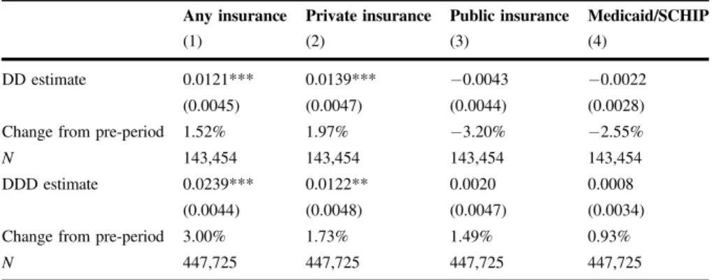
were the main reason for why many workers decided not to enroll in insurance plans that they were offered. Previous work has shown that higher EITCs increase private and employer-sponsored insurance coverage (Baughman and Duchovny 2016; Hoynes et al.2015; Baughman 2005). While the studies by Baughman and Duch-ovny (2016) and Hoynes et al. (2015)find that these increases are offset by reduction in public insurance, switching to potentially more comprehensive plans could be a potential mechanism underlying the link between the EITC and health. This study also examines the role of health insurance in explaining potential changes in health outcomes following the expansion of the EITC by estimating the effects on overall coverage as well as on different insurance types. Given that the HITC, which was only in place until 1993, had very low take-up rates, and had the same eligibility criteria for households with one or at least two children, the insurance estimates should not be affected by the HITC. To check for this, I re-estimate the insurance effects when leaving out the years prior to 1994 in additional specifications.
Third, increases in income as well as income security might lead to changes in health-related behaviors, such as timely receipt of medical, and changes in smoking and drinking, which in turn influence health outcomes for children and adults. Averett and Wang (2013) and Hoynes et al. (2015) show that the federal expansion in the EITC reduced smoking among mothers. However, in a longitudinal study of New Zealand’s Family Tax Credit, Pega et al. (2017) find no relationship between the cumulative receipt of the credit and tobacco smoking. Cigarettes and alcohol are typically found to be normal goods (i.e., the amount purchased rises with increased income) and therefore higher incomes could also be associated with more smoking and drinking (Kenkel et al.
2014). This could have deleterious effects on health outcomes.
Fourth, closely related to changes in health-related behavior, increases in the EITC likely reducesfinancial stress and increases income security of families. Evans and Garthwaite (2014) show that expansions of the federal EITC not only improved self-reported health but also lessened the count of risky biomarkers in low-educated mothers, indicating reductions in stress. Early research in the medical literature documents the presence of physiological reactions to stress in the form of heart diseases and problems with the circulatory system (Sterling and Eyer1981; Henry
1982). Thus, changes in stress can be another mechanism through which the income affects health outcomes. Lenhart (2017) provides suggestive evidence that increases in wages reducefinancial stress and improve health outcomes of low-wage workers in the UK.
While this paper focuses on estimating the effects on increased EITC benefits on health status of affected heads of households, I believe that testing for changes in food expenditures and health insurance coverage can provide policy implications with respect to the health of all household members. It seems likely that all members of the household will be affected by potential increases in food expenditures. Similarly, children would also benefit from increased insurance coverage or switches from public to private by the head of the household.
3.3 Other welfare reforms during the 1990s
The late 1990s witnessed significant changes in welfare policies due to the imple-mentation of the Personal Responsibility and Work Opportunity Reconciliation Act
(PRWORA). The main goal of the reforms was to make low-income families independent of welfare benefits and to provide states withflexibility in determining eligibility criteria and benefit levels. Previous literature has established that the policy changes significantly affected the lives of lower-income families who were depen-dent on welfare assistance at the time (Schoeni and Blank2000). A relatively small number of studies have so far examined whether the welfare reforms affected health outcomes of affected individuals. Using data from the Survey of Income and Pro-gram Participation (SIPP), recent work by Narain et al. (2017) provides suggestive evidence that PRWORA led to a 7-percentage point increase in the probability with which low-educated white single mothers report to be in poor health. By examining changes to time limits in Florida during the 1990s, Muennig et al. (2013) provide evidence that certain aspects of the welfare reforms can lead to increased mortality rates. Thesefinding differ from results obtained by earlier studies, which showed that the welfare reforms had very little effects on birth weight (Kaestner and Lee2005), physical health outcomes (Bitler et al.2005; Kaestner and Tarlov2006) as well as mental health (Kaestner and Tarlov 2006). Bitler et al. (2005) furthermore find reductions in preventative care following the introduction of the reforms, while Kaestner and Tarlov (2006) show that declines in welfare caseloads in the late 1990s reduced binge drinking, but were not associated with changes in smoking, nutritional intake, and exercising.
As mentioned by Evans and Garthwaite (2014), other welfare changes that occurred in the 1990s offer a threat to the estimating the effects of the EITC expansion on health outcomes if those changes differentially affected low-income families with two or more children compared to families compared to families with only one child. The authors point out that, in general, welfare reform should affect low-income mothers with one and two children to similar degrees. One advantage of the timing of the EITC expansion examined in this study is that it was implemented two years before thefirst welfare reforms were passed, which allows separating the effects of the policy changes to some extent. Given that statefixed effects can only deal with the state-level heterogeneity that is time-invariant, including them in the specifications is not sufficient to account for statewide variations in welfare reforms. To account for other policy changes that occurred during the period of this study, all main models are re-estimated when controlling for a set of state-specific character-istics and welfare policy variables. These include information on statewide variations in welfare eligibility thresholds, waivers, sanctions, and time limits, as well as in Medicaid expansions. Finally, these models also control for state-level unemploy-ment rates and whether state-level EITC benefits are in place on top of the federal credit (please see the full list of additional control variables in the Appendix).
4 Data
4.1 Panel study of income dynamics (PSID)
The main part of this study uses data from the Panel Study of Income Dynamics (PSID), a nationally representative longitudinal sample of households and families interviewed annually since 1968 and biannually since 1997. The study uses data for
the years 1990 to 2003, which provides the analysis 11 years of data. The PSID, the longest running U.S. panel, was specifically designed to track income dynamics over time. The survey over-samples low-income families, which is advantageous for this analysis since these households are more likely to be eligible to receive EITC. Due to its detailed information on earnings, the PSID is well-suited for calculating simulated EITC benefits through the tax simulator program NBER TAXSIM (version 9; for more information see Feenberg and Coutts 1993). Furthermore, by using state identifiers provided in the PSID, I am able to simulate both state-level and federal EITC benefits.3
In order to obtain treatment effects on the treated, the sample is limited to heads of households with at least one child who, based on the TAXSIM simulations, are eligible to receive EITC benefits.4Consistent withfindings in the literature showing that 80–87% of eligible households indeed receive the credit (IRS 2002; Scholz
1994), this study assumes full take-up rates (Dahl and Lochner 2012). Individuals with missing income information (5.4% of the sample) are dropped from the analysis since the use of imputed values could cause a substantial measurement error and attenuate the estimates. Throughout the period of the study, there are no differences in the share of individuals with missing income information among those that are affected by the EITC expansion and those that are not. Given that missing income values are non-random, large differences between the two groups would cast some concerns about the obtained estimates. Heads of households with missing informa-tion on their health status are removed from the analysis as well, whereas the sample is restricted to individuals less than 65 years of age.5
The main dependent variable is self-reported health status, which is categorized on a scale from 1 (excellent) to 5 (poor). Self-assessed health has been widely used in previous studies regarding the relationship between income and health (e.g., Case et al.2002; Currie and Stabile2003; Adda et al.2009). It has been shown to be a good predictor of other health outcomes, including mortality (Idler and Benyamini
1997), future health care usage (van Doorslaer et al.2000) and future hospitalizations (Nielsen 2016). The longitudinal nature of the PSID reduces the potential mea-surement error in the self-reported health variable in two ways: (1) by comparing each individual’s health only to their own prior assessment, and (2) by controlling for the fact that each respondent may have their own scales in ranking their health (reference bias). Additionally, the panel nature of the PSID allows me to account for potential changes in the composition of the sample following the increase of EITC benefits.
3 The EITC values are calculated based on a family
’s earnings in the previous year and federal and state EITC laws for the number of eligible children. Details are available upon request.
4 The simulated EITC bene
fits obtained through the simulation program are based on up to 22 categories, including previous years’income and other types of earnings. For more information, please see Feenberg and Coutts (1993).
5 Dropping individuals with missing self-reported health information in some years of the analysis could
bias the results if these respondents were different from the remaining sample, for example in terms of health. Appendix Table A1 shows that there are relatively small differences between the samples with and without missing self-reported health information. The statistics shown in Table A1 are obtained using the sample of people eligible to receive EITC benefits throughout the sample period. The descriptive statistics are similar for the other two samples used in this study.
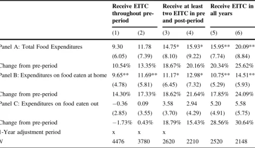
When testing for the role of food expenditures as a channel underlying the rela-tionship between income and health, the dependent variables are the amounts of money that a household spends on food per week. Additionally, I examine whether any potential changes are driven by people purchasing more food that is eaten at home or away from home.6Despite the fact that spending more money on food does not guarantee that individuals buy groceries with higher quality, I believe that increases in food expenditures can be viewed as a proxy for an increase in food quality. Consistent with this, a study by McGranahan and Schanzenbach (2013) provides evidence that EITC receipt increases spending on relatively healthy gro-ceries while lowering expenditures on processed fruit and vegetables.
4.2 Current population survey (CPS)
Besides examining the role of food expenditures, this study also tests for the role of health insurance coverage as a potential mechanism underlying the relationship between income and health. For this analysis, I use data from the annual March Population Survey (March CPS). In order to narrow the sample down to individuals who are eligible to receive EITC payments, I again use the TAXSIM program to obtain predicted amounts of EITC benefits.7Using March CPS data in order to test for the role of insurance is beneficial since it provides extensive information on the health insurance coverage. More specifically, I test for the effect of the expansion of the EITC on different types of insurance (private, public, Medicaid/SCHIP). Besides examining whether individual are more likely to have insurance coverage following an increase in income, this also allows testing whether individuals switch between different types of plans after the policy change following increases in income. Since information on insurance coverage is only available from 1992 and onwards, the period of interest is reduced to the years 1992 to 2000.
4.3 Descriptive statistics
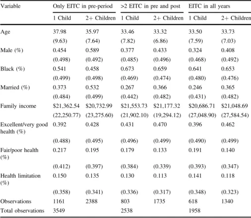
Table2 presents descriptive statistics for the three samples that are analyzed in the study. On average, heads of EITC-eligible households with at least two children are more likely to be male and married, while those with one child are slightly older in the least restricted sample (only EITC in pre-period). A potential explanation for the gender differences across the two groups is that single mothers represent 31% of EITC recipients and 41% of EITC funds (Meyer2007). According to the statistics in Table2, it seems that EITC-eligible single mothers in the sample are more likely to have one child. Family incomes are relatively similar for the groups. The bottom of Table2 shows summary statistics for health-related outcomes. It is noticeable that 6 The PSID provides data for these outcomes starting in 1994. The survey questions do not include meals
eaten at work or at school.
7 The March CPS also provides its own simulated EITC payments using the Census Bureau
’s tax model, which simulates individual tax returns to produce estimates of federal, state, and payroll tax amounts by incorporating information from non-CPS sources such as the Internal Revenue Service’s Statistics of Income series, the American Housing Survey and the State Tax Handbook. To be consistent with the previous analysis, I use the TAXSIM simulations for the CPS data when examining the role of health insurance. However, the results are unchanged when using the CPS simulations.
heads of households with more than one child are, on average, in better self-reported health than those with one child. Figure1shows changes in the share of individuals who report either excellent or very good health across during the period of the study for the sample of individuals that were eligible to receive EITC benefits throughout the pre-expansion period.8The graph provides evidence that, while health status was relatively similar for the two groups before the policy change, individuals with two or more children are more likely to report being in either excellent or very good health following the expansion of the EITC.
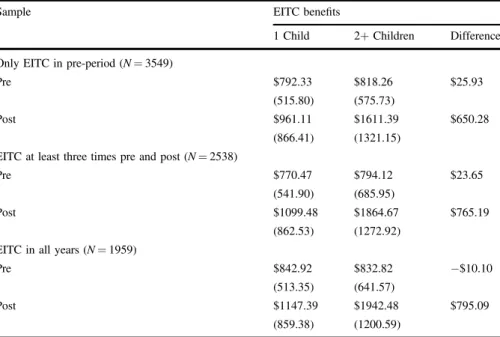
Table 3 provides descriptive statistics for the amount of EITC received by households with one and at least two children before and after the EITC expansion. Statistics for three different sample are presented, that differ in how restrictive the sample is selected. For all three Panels (A, B, and C), it is observable that there were very small differences in EITC benefits for eligible families from the two groups prior to the policy expansions. After the implementation of the policy change, however, families with two or more children receive substantially higher payments than those with only once child. The differences in EITC benefits between the two groups following the reform are larger than found by other studies. For example,
Table 2 Descriptive statistics for eligible heads of households (PSID)
Variable Only EITC in pre-period >2 EITC in pre and post EITC in all years 1 Child 2+Children 1 Child 2+Children 1 Child 2+Children Age 37.98 35.97 33.46 33.32 33.50 33.73 (9.63) (7.64) (7.82) (6.86) (7.59) (7.03) Male (%) 0.454 0.589 0.377 0.433 0.324 0.408 (0.498) (0.492) (0.485) (0.496) (0.468) (0.492) Black (%) 0.541 0.458 0.673 0.659 0.641 0.653 (0.499) (0.498) (0.469) (0.474) (0.480) (0.476) Married (%) 0.373 0.532 0.267 0.366 0.246 0.365 (0.484) (0.499) (0.442) (0.482) (0.431) (0.482) Family income $21,362.54 $20,732.99 $21,553.73 $21,177.32 $20,686.71 $21,048.69 (22,250.77) (23,275.60) (21,902.10) (19,294.12) (27,048.90) (27,584.54) Excellent/very good health (%) 0.392 0.428 0.431 0.470 0.396 0.462 (0.488) (0.495) (0.496) (0.499) (0.490) (0.499) Fair/poor health (%) 0.217 0.195 0.179 0.133 0.191 0.140 (0.412) (0.397) (0.384) (0.339) (0.393) (0.347) Health limitation (%) 0.150 0.135 0.130 0.113 0.141 0.118 (0.358) (0.341) (0.336) (0.317) (0.348) (0.323) Observations 1161 2388 803 1735 618 1340 Total observations 3549 2538 1958
8 The graphs looks very similar for the other two samples. They are not shown in the paper due to space
Averett and Wang (2013)find a gap $320 in benefits between families with one or at least two children. I believe the reason for the larger differences in my analysis is the fact that, rather than focusing on individuals with at most a high school degree, I select my sample based on TAXSIM information indicating which households are eligible to receive EITC credits in a given years,
Consistent with Table3, Fig.2provides graphical motivation for using the EITC expansion to examine the causal link between income and health. The picture shows
Fig. 1Share of eligible heads of households in excellent/very good health. Figure1shows the average share of individuals in both groups who report either excellent or very good health for the sample of individuals that received EITC benefits throughout the pre-expansion period
Table 3 Effect of the policy on EITC (PSID Data)
Sample EITC benefits
1 Child 2+Children Difference Only EITC in pre-period (N=3549)
Pre $792.33 $818.26 $25.93
(515.80) (575.73)
Post $961.11 $1611.39 $650.28
(866.41) (1321.15) EITC at least three times pre and post (N=2538)
Pre $770.47 $794.12 $23.65
(541.90) (685.95)
Post $1099.48 $1864.67 $765.19
(862.53) (1272.92) EITC in all years (N=1959)
Pre $842.92 $832.82 −$10.10
(513.35) (641.57)
Post $1147.39 $1942.48 $795.09
the amount of EITC which eligible families in the sample receive (in 1999 dollars) for the sample of individuals that receive EITC benefits in all years of the sample. Again, while only small differences in EITC benefits are observable before the expansion for families with one child and those with two or more children, the gap becomes large in the years after the policy change. By 1999, the difference between the two groups is about $900 and it remains very similar for the remaining years.
5 Econometric models
5.1 DD models
The study exploits the expansions of the EITC through OBRA 1993 in order to test for a causal relationship between income and health outcomes. The structure of the policy changes offers the opportunity for a difference-in-differences (DD) framework to observe the average treatment effects. In the presence of changes in the compo-sition of the sample, a cross-sectional analysis could provide inaccurate estimates if healthier individuals with two or more children choose to enter the labor force following the incentives of being eligible to higher EITC benefits after the policy change. Thus, the main specification of this paper uses the longitudinal nature of the PSID to control for individualfixed effects and to purge the estimates of individual time-invariant heterogeneity. I examine treatment effects for three different specifi -cations, which differ in how restrictive the sample was selected: (1) examines all individuals that were eligible to receive EITC benefits in all years before the policy change; (2) examines all individuals that were eligible to receive EITC benefits in at least three years both before and after the policy change; (3) examines individuals who are eligible to receive EITC benefits throughout the sample period. Since it has been shown that the EITC is often more a short-term safety net for low-income families, the number of observations in the third sample is relatively small. For all
Fig. 2 The size of EITC credits for eligible households (in 1999 $). Figure2shows the average real dollar amounts of EITC which individuals from both groups are eligible to receive benefits based on the TAXSIM simulations
three samples, I estimate the following equation:
Yit¼β0þβ12KIDSitþβ2XitþδDDPOSTit2KIDSit þλ1Yearþλ2Stateþαiþεit;
ð1Þ
whereYitis an indicator that equals one if the EITC-eligible respondent reports to be in either excellent or very good health; 2KIDSitequals to one if there is more than one eligible child in the household; and POSTitis an indicator for the time period either before or after 1996. As shown in Table 1, the EITC expansions through OBRA 1993 were slowly phased in over the tax years 1994 and 1995. Evans and Garthwaite (2014) mention that a potential misclassification of individuals who are treated in the pre-treatment period should bias the observed estimates in this study againstfinding any health impacts. For additional robustness, I re-estimate the main models when allowing the post-treatment periods to start in 1994 and 1995, respectively. While accounting for individual time-invariant heterogeneity, the longitudinal nature of the data will not remove any potential bias in case there is a causal pathway from health to employment. In order to check for this potential pathway, I additionally estimate three specifications examining the presence of reverse causality as robustness checks.
Households in which changes in the number of children during the sample period move them from the control to the treatment group are dropped from the analysis, which is consistent with previous work using longitudinal data by Averett and Wang (2013). In a later robustness check, I include the 28 individuals who switched between groups during the sample period.Xitrepresents a set of baseline covariates that include controls for age and marital status of the head of household as well as the number of children in the household.δDD is the main parameter of interest, which captures the effect of the EITC expansion on the health status. αi captures the
individual fixed effects or unobserved time-invariant heterogeneity across indivi-duals. A set of year and state dummy variables are controlled for to accounts for differences in health patterns across time and states. The state fixed effects are important to control for existing differences across states. To further account for other welfare reforms that were passed in the late 1990s in the US, I also estimate specifications that net out the effects of several time-varying differences across states in labor market and welfare reforms (Averett and Wang2016). I use linear prob-ability methods to estimate the main specifications shown in this section. In addi-tional specifications, I examine whether the effects change when allowing the policy change to have a 1-year adjustment period after its implementation. It seems rea-sonable to assume that it might take some time before health outcomes are affected by increases in income. In these specifications, observations from the year 1996 are omitted from the analysis.
One downside of using simulated EITC benefits to create the sample is that families are not randomly distributed by health into the income ranges that would or would not make them eligible for the EITC. Poor health makes employment, which is required for at least one member of the household in order to receive any benefits, less likely. Furthermore, fully-informed families could manipulate their incomes to maximize their EITC benefits. I use two approaches to reduce potential concerns about the endogeneity of predicted EITC eligibility. First, as mentioned above, I use longitudinal data and estimate treatment effects for three different samples that vary
by the level of restrictiveness. The narrowest sample consists of individuals who were eligible to receive EITC benefits throughout the period of the study. Given that these people had no foresight about the policy changes at the beginning of the study, this sample should account for potential changes in the composition of the sample due to incentives provided by the expansion. The fact that the gap in EITC benefits between treatment and control group for the most restrictive sample (shown in Fig.1) is consistent with the actual differences in benefits due to the expansion (Table 1) provides further suggestive evidence that the individuals who are followed throughout all years of the sample period did not manipulate their incomes to increase their benefits.
Second, I estimate whether the policy change affected the control variables used in the main specification (gender, race, marital status, education). The main treatment effect estimates could be biased if individuals who are eligible to receive EITC benefits both before and after the policy change are more likely to benefit from income increases, which would be the case if their health were more susceptible to changes in income. I re-estimate equation (1) with the main control variables as the outcomes. The results show that the policy change does not significantly affect any of the observable characteristics.9
5.2 DDD models
Like any DD model, the estimation of equation (1) makes the key assumption that trends in health outcomes over time are similar across both the treatment and control groups. While there appears to be no obvious reason to expect that this assumption is not satisfied in the given framework, a violation would lead to a bias ofδDD. One way to reduce this potential bias is to explore a difference-in-difference-in-differences (DDD) framework. The additional comparison groups consist of households with children (one and at least two) who are, based on the tax simulations, not eligible to receive EITC benefits in any year point during the study period (1990 to 2003). The estimated equation in the DDD model is the following:
Yit¼β0þβ1POSTitþβ22KIDSitþβ3ELIGitþβ4POSTit2KIDSit þβ5POSTitELIGitþβ6ELIGit2KIDSitþβ7XitþδDDDPOSTit
ELIGit2KIDSitþλ1Stateþαiþεit;
ð2Þ
where ELIGit is an indicator for whether a family is eligible to receive any EITC benefits during the year of the survey.δDDDis now the parameter of interest, whereas the other variables remain the same as in equation (1).
Given that the lack of eligibility benefits is likely to more endogenous, I also estimate the fixed effect DDD model by using education as the criteria for being eligible to receive benefits. This follows the DDD setup by Averett and Wang (2013) who use longitudinal data as well to estimate the effects of EITC expansions on smoking of mothers. Individuals with at least 13 years of education with children (one and two or more) form the additional comparison groups, who are likely to be ineligible for EITC benefits, while heads of households with children (one and two or 9 These results are not shown in the paper, but are available upon request.
more) with no more than 12 years of education form the main treatment and control group for this specification.
5.3 Additional models
This section introduces two additional models, which I estimate to test whether the main results are robust to other model specifications. First, I conduct a falsification test that compares the health outcomes of heads of households from two groups that are equally affected by the policy change. During the period of my study, there were no differences in EITC benefits for families with more than one child. Only following the implantation of the American Recovery and Reinvestment Act (ARRA) in 2009, benefits for eligible families with three or more children increased significantly. Following the falsification test conducted by Averett and Wang (2013), eligible heads of households with two children form the control group for this specification, while those with at least three children form the treatment group. Everything else in the falsification test is the same as equation (1). Finding no differences in health outcomes between these two groups can provide evidence that the main analysis is actually capturing health effects due to of the EITC policy change and not due to other time-varying factors that could be correlated with health status (Averett and Wang2013). Figure3confirms the validity of the falsification test by showing that that EITC credits evolved identically throughout the period of the study for eligible households with two and three or more children.
Second, I estimate a semi-parametric DD model, which was introduced by Abadie (2005) and which relaxes the assumption of a linear relationship between income and health. The method captures average treatment effects for the treated group (ATT) for the case that differences in observed characteristics create non-parallel outcome dynamics between the two observed groups, which violates the main assumption of
Fig. 3 EITC Benefits to Eligible Households with 3+Children vs. 2 Children. Figure3shows the average amounts of EITC, which individuals from the groups used in the falsification test, are eligible to receive benefits based on my TAXSIM simulations
standard DD models. The ATT is given by the following equation: E Y 1ð Þ1 Y0ð Þ1 jD¼1 ¼E P Dð ¼1jXÞ P Dð ¼1Þ φ0Y ; ð3Þ
where Y(1) and Y(0) represent health outcomes before and after the treatment, D is an indicator for belonging to the treatment group, P(D=1) gives the probability of receiving treatment, and P(D=1 | X) is the propensity score that equals the probability of treatment, conditional on the observed covariates X. The propensity scores for the semi-parametric analysis are obtained using probit estimation.10The value ofφ0is obtained from the following equation:
φ0¼ T γ
γ ð1 γÞ
D P Dð ¼1jXÞ
P Dð ¼1jXÞ P Dð ¼0jXÞ; ð4Þ
where T is a time indicator that equals one if the observation belongs to the post-treatment period andγreflects the proportion of observations sampled in the
post-treatment period. Abadie (2005) shows that the semi-parametric estimator is obtained through two steps: (1) Estimation of the propensity score and computation offitted values for the sample; and (2) Plugging in the obtainedfitted values into the sample analogue of equation (4) to obtain average treatment effects for the treated. According to Abadie (2005), simple weighted average differences in the outcome of interest over time can recover estimates for treatment effects, while the weights depend on the propensity scores. This guarantees that the same distribution of covariates is imposed for the treatment and for the control group. The average estimatedfitted values for the sample is 0.6207.11
6 Results
6.1 DD estimation
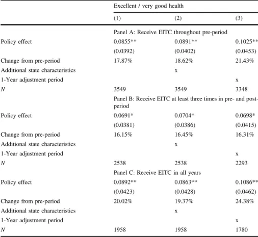
Table4 reports the DD fixed effect estimates of the impact of receiving additional income through the EITC expansion on the health outcomes of heads of households. The main dependent variable is a binary indicator that equals 1 if an individual reports being in either excellent or very good health. Consistent with the descriptive statistics shown in Tables2and3, estimates for three different samples are presented. Panel A shows DD results for the sample of individuals that were eligible to receive EITC benefits throughout the pre-treatment period (1990 to 1995). The baseline estimate in column (1) suggests that being eligible for the increased benefits raises the likelihood of being in the top two health categories by 8.55 percentage points (p
< 0.05). This effect corresponds to a 17.87% change from the pre-treatment period. When additionally accounting for state-specific controls in column (2), the result 10I additionally re-estimate the propensity scores using the two other commonly used estimation
tech-niques for propensity scores, logit and cloglog estimation. The results remain unchanged.
11Histograms of the propensity scores for the pre- and post-policy period provide evidence that there is a
common support for the groups in both periods. The histograms are not shown in the paper, but are available upon request.
remains almost unchanged, which supports the claim that the health effects are not spuriously driven by the other safety net laws passed during the 1990s. Table A2 in the Appendix provides the estimates for these additional state characteristics that can capture the role of welfare reforms on health status. While no statistically significant effects are noticeable for any of the welfare reform controls, the effects shown in Table4 could potentially be lower bound effects since previous work has provided evidence for negative effects of welfare reform on health (Muennig et al. 2013; Narain et al.2017). Table A2 also shows that Medicaid expansions have a negligible effect on health status and that controlling for them does not alter the main estimates. As suggested by Fig.1, the effect of receiving afinancial boost on health status becomes larger once the DD model allows the EITC expansion to have an adjustment period shortly after its implementation. This seems reasonable since it might take
Table 4 Fixed effect DD estimates for the effects of EITC expansion on health status (PSID data) Excellent / very good health
(1) (2) (3)
Panel A: Receive EITC throughout pre-period
Policy effect 0.0855** 0.0891** 0.1025** (0.0392) (0.0402) (0.0453) Change from pre-period 17.87% 18.62% 21.43% Additional state characteristics x
1-Year adjustment period x
N 3549 3549 3348
Panel B: Receive EITC at least three times in pre- and post-period
Policy effect 0.0691* 0.0704* 0.0698* (0.0381) (0.0386) (0.0415) Change from pre-period 16.15% 16.45% 16.31% Additional state characteristics x
1-Year adjustment period x
N 2538 2538 2293
Panel C: Receive EITC in all years
Policy effect 0.0892** 0.0863** 0.1086** (0.0423) (0.0428) (0.0462) Change from pre-period 20.02% 19.37% 24.38% Additional state characteristics x
1-Year adjustment period x
N 1958 1958 1780
Robust standard errors, clustered by states, are shown in parentheses. All models control for age, marital status as well as the number of people living in the household. Furthermore, individual, state and yearfixed effects are controlled for. The additional state characteristics include average annual state unemployment rates, state-level AFDC eligibility requirements (for a family of three), the presence and timing of AFDC waivers and time limits on receiving welfare, the type of sanctions as well as whether the state expanded Medicaid coverage and implemented state-level EITC benefits
some time before health impacts of the extra income become noticeable. Column (3) confirms this by showing a treatment effect of 10.25 percentage points (p< 0.01) when a 1-year adjustment period is considered following the policy change.12
Panel B and C show estimates from sample of households that are eligible to receive EITC benefits at least three times in both the pre- and the post-treatment period as well as for households that are eligible to receive benefits throughout the sample period, respectively. The estimates in Panel B confirm the positive effect of the EITC expansion on health of affected heads of households. The analysisfinds a 6.91 percentage point (p< 0.10) increase in the likelihood of reporting excellent or very good health status following the policy change, which corresponds to a 16.15% change. The largest observed effects are observed when using the most restrictive sample selection by only including households that receive EITC benefits throughout the study period (Panel C). The effects found range from 8.92 percentage points (p< 0.05) in the baseline specification to 10.86 percentage points (p< 0.05) when allowing the policy change to adjust for one year. Given how restrictive the sample is selected in Panel C, it seems intuitive that the largest treatment effects are found in this sample since it is closest to providing treatment effects on the treated instead of estimating intent-to-treat effects.13Table A3 and A4 in the Appendix shows that the results remain consistent when estimating ordered logit models using the entire distribution of health outcomes and when moving the start of the post-treatment to 1994 and 1995. These results provide additional robustness to the mainfindings of Table4.
In their work on the Oregon Health Insurance Experiment, Finkelstein et al. (2012)find that low-income adults who gained Medicaid coverage through the lot-tery are significantly more likely to report better physical health in the year after the lottery. Given the magnitude of their results and the short time frame before these effects are observed, the authors suggest and provide preliminary evidence that they might to some extent reflect improvements in general well-being. Finkelstein et al’s (2012) LATE estimate indicates a 24.3 percent increase in the likelihood of reporting excellent, very good or good health status. The treatment effects observed in this study are similar in magnitude. Across the three samples used in the main DD models (Table4, Column 1), the estimates suggest that the likelihood of reporting excellent or very good health status increased by between 16.2 to 20.0% compared to before the policy change. Unlike Finkelstein et al. (2012), the estimates of this study provide average treatment effects for a period of eight years after the policy change. While Fig.1suggests that the changes in health are more pronounced several years after the
12In additional models, I test for the effects of the policy on the likelihood of reporting fair or poor health.
Whilefinding negative effects, the estimates for the bottom two categories of health status are smaller in magnitude than the estimates for the top two health categories (reduction of 4.02 percentage points compared to an increase of 8.55 percentage points), while also being imprecisely estimated. One reason for the relatively smallfinding could be that only 14.91% of treated individuals report being in the bottom two health categories prior to the policy change. Thus, while lacking statistical significance, the observed decline of 4.02 percentage points corresponds to a 26.96% change, which is even larger than the change in the top two categories of health status.
13In additional speci
fication, I estimate treatment effects separately for males and females. The results suggest that the positive effects of income on health are larger for women than for men. These results are not shown in the paper, but are available upon request.
EITC expansion, it should be noted that the effects could to some extent reflect that affected individuals are simply happier following the change in the EITC.
6.2 DDD estimation
The previous estimates remain unbiased if similar health trends would have occurred for individuals in both the treatment and control groups in the absence of the policy change. Figure 2 provides suggestive evidence supporting this assumption by showing that trends in health status were similar in most years before the policy implementation. To further account for potential differences in health trends between households with two or more children and those with one child, I additionally estimate Difference-in-Difference-in-Differences (DDD) models, which include heads of households with children who are not eligible to receive EITC benefits as an additional comparison group.
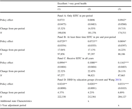
DDD estimates for the impact of the policy change on health are presented in Table 5. It is noticeable that the results are fairly consistent with the DD effects shown in Table4. While the results for the sample of households that were eligible to receive EITC benefits throughout the pre-treatment periods are slightly smaller in magnitude (Panel A), the observed effects for the other two samples are actually slightly larger than the DD results. Finally, Panel D provides DDD estimates from using education as the main criteria for EITC eligibility (Averett and Wang2013). While substantially smaller in magnitude, the estimate also show that the policy change increases the likelihood of being in excellent or very good health. Overall, the
findings in Table5confirm that the observed positive effects of additional income on health status remain when accounting for potential differential health trends between households forming treatment and control groups and remove concerns that the DD results might be biased.
6.3 Robustness checks
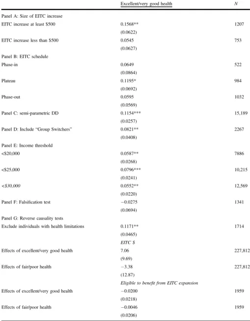
In order to further test for the validity of the main results of the study, estimates for several additional robustness checks are presented in Table6. First, I use the amounts of predicted EITC dollars that are obtained from the tax simulator in order to check whether health effects as a result of the expansion were larger for individuals who received higher EITC benefits. The results in Panel A indicate that the effect of additional earnings on health status is substantially stronger for treated individuals who received larger EITC payments (p < 0.05). This finding provides additional evidence for the positive link between income and health.14
In Panel B, I use family income and EITC schedules for the study period to identify where in which part of the EITC schedule households are. This allows me test whether the effects on health differ across the phase-in, the plateau and the phase-out region. Previous research on the program has established that households 14In an additional speci
fication, I test for the effect of annual changes in predicted EITC benefits on health status. While the estimates suggests that higher increases in EITC have positive health effects, they are imprecisely estimated. One reason for this could be that overall there is relatively small variation in EITC payments to the two groups (on average $113 per year for the entire sample period), with substantial changes only occurring around the time of the EITC expansion.
in the phase-in part of the schedule increase their employment on the extensive margin following changes to the EITC (Eissa and Liebman1996; Eissa et al. 2008; Meyer 2010). On the other hand, earlier work has shown that household in the middle of the schedule receiving something close to a pure income effect because of little to no change in the number of hours worked (Athreya et al.2010; Gunter2013). To my knowledge, no previous study has examined whether the effects of EITC changes on health outcomes differ across the three parts of the schedule. The esti-mates in Panel B show that individuals in the plateau phase experienced the largest improvements in health status (p< 0.10), while the effects are smaller in magnitude and imprecisely estimated in both the phase-in and phase-out part of the schedule. Again, the findings provide additional evidence that the improvements in health following the EITC expansion, which are shown in the main analysis, are the result of increases in income.
Panel C presents estimates from the semi-parametric DD model, which was introduced by Abadie (2005). The results are consistent with the main estimates shown in Table4, with the observed effects being larger in magnitude. The policy change is shown to increase the likelihood of reporting excellent or very good health
Table 5 Fixed effect DDD estimates for the effects of EITC expansion on health status (PSID data) Excellent / very good health
(1) (2) (3)
Panel A: Only EITC in pre-period
Policy effect 0.0733 0.0696 0.0943* (0.0475) (0.0483) (0.0560) Change from pre-period 15.32% 14.55% 19.71%
N 190,036 181,376 174,511
Panel B: At least three time EITC in pre and post-period Policy effect 0.0729** 0.0733** 0.0694*
(0.0354) (0.0355) (0.0397) Change from pre-period 17.04% 17.13% 16.22%
N 97,856 97,397 88,186
Panel C: Receive EITC in all years
Policy effect 0.0994** 0.1000** 0.1163*** (0.0404) (0.0404) (0.0403) Change from pre-period 22.32% 22.45% 26.11%
N 97,277 96,821 87,663
Panel D: DDD by education groups(Averett and Wang2013)
Policy effect 0.0210** 0.0203** 0.0331*** (0.0090) (0.0091) (0.0103) Change from pre-period 4.37% 4.23% 6.89%
N 222,330 212,561 204,127
Additional state Characteristics x
1-Year adjustment period x
Robust standard errors, clustered by states, are shown in parentheses. All models control for age, marital status as well as the number of people living in the household. Furthermore, individual, state and yearfixed effects are controlled for
Table 6 Robustness checks
Excellent/very good health N
Panel A: Size of EITC increase
EITC increase at least $500 0.1568** 1207 (0.0622)
EITC increase less than $500 0.0545 753 (0.0627)
Panel B: EITC schedule
Phase-in 0.0649 522 (0.0864) Plateau 0.1195* 984 (0.0692) Phase-out 0.0595 1032 (0.0569) Panel C: semi-parametric DD 0.1154*** 15,189 (0.0257)
Panel D: Include“Group Switchers” 0.0821** 2267 (0.0408)
Panel E: Income threshold
<$20,000 0.0587** 7886 (0.0268) <$25,000 0.0796*** 10,215 (0.0241) <$30,000 0.0552** 12,569 (0.0220)
Panel F: Falsification test −0.0275 1341
(0.0694) Panel G: Reverse causality tests
Exclude individuals with health limitations 0.1171** 1714 (0.0465)
EITC $
Effects of excellent/very good health 7.06 227,812 (9.69)
Effects of fair/poor health −3.38 227,812
(12.87)
Eligible to benefit from EITC expansion
Effects of excellent/very good health −0.0200 1959
(0.0218)
Effects of fair/poor health −0.0046 1959
(0.0206)
Robust standard errors, clustered by states, are shown in parentheses. All models control for age, marital status as well as the number of people living in the household. Furthermore, individual, state and yearfixed effects are controlled for. The estimate in Panel D is obtained using the most narrow sample selection and is therefore comparable to the estimate in Table3, Panel C, column (1)