Testing for the Extent of Competition Among Banks in the
Southern African Development Community (“SADC”) Region
Dikabelo Mashego
March 2015
DECLARATION
I hereby declare that this thesis is my own work and effort and that it has not been submitted anywhere for any award. Wherever contributions of others are involved, effort was made to
indicate this clearly, with suitable reference to literature.
The work was done under the supervision of Tendai Gwatidzo of the University of Witwatersrand.
………. Dikabelo Mashego
……… Date
Testing for the Extent of Competition Among Banks in the SADC
Region
Abstract
This paper analyses the competitiveness in the banking sector of eight countries in the SADC region. Both the Panzar-Rosse and the Lerner Index approaches were used for the period 2002- 2013. Although the results yield opposing outcomes, the overall findings suggest that the eight countries cannot be described as being perfectly competitive but rather suggest imperfect competition in these banking sectors. These countries could be characterised as monopolies when using the Panzar-Rosse study and monopolistically competitive when using the Lerner Index.
Table of Contents
1. INTRODUCTION ... 1
2. OVERVIEW OF BANKING SECTOR IN THE SADC REGION ... 3
3. LITERATURE REVIEW ... 5 3.1 THEORETICAL LITERATURE ... 5 3.2 EMPIRICAL LITERATURE ... 7 4. DATA ... 9 5. METHODOLOGY ... 9 5.1 PANZAR-ROSSE APPROACH ... 10 5.2 LERNER INDEX ... 11 6. EMPIRICAL RESULTS ... 12 6.1 PANZAR-ROSSE ... 12 6.2 LERNER INDEX ... 21 6.3 ROBUSTNESS CHECKS ... 27 7. CONCLUSION ... 27 8. APPENDIX ... 29 9. REFERENCES ... 38
1.
Introduction
The Southern African Development Community (“SADC”) exists to liberalise the economies of its region in an attempt to improve livelihoods of the people of Southern Africa. It is for this reason that it strives to build an efficient integrated banking system that will better facilitate trade among member countries and with the rest of the world.
Over the years, African banking systems have experienced significant transformations following long periods of underperformance. For instance, open market operations have replaced interest rate controls in countries like Kenya, Ghana and Tanzania, as well as directed lending in Uganda (Fosu, 2013). Another area of change within each sub-region is the significant privatisation of state-owned banks (for example Kenya, Uganda, Tanzania and Zambia) as an attempt to minimise inefficiencies. Furthermore, in response to increased regional integration and advances in information technology, there has been a significant upward trend in cross-border banking allowing customers to operate their accounts outside their home country (Fosu, 2013). These reforms have implications for the banking sector, competition in particular. It is believed that sufficient competition among banks will significantly improve stability in the banking sector. A competitive banking sector is understood to be more efficient, in terms of delivery, for the users of bank services. Restraining competitive pressures can result in welfare losses (Cetorelli, 2001). Banks with monopoly power are more likely to charge higher interest rates and prices to clients while lowering rates of return to depositors. Higher rates discourage entrepreneurial incentives to undertake risky yet profitable projects and limit small firms from accessing financial capital, weakening the stability of credit markets further. Without competitive pressures banks limit technological innovation and productivity within the financial sector- creating inefficiency problems. This can slow economic growth of a country. Economic growth is crucial for the SADC countries if they are to meet their targeted goals of improving the wellbeing and the overall standard of living of their citizens.
Various fiscal and monetary policies are implemented in order to achieve the targeted goals. However, these policies are not distinct from the banking structure of an economy. There are inconsistencies between the effects of monetary policy shocks on economies with different competitive banking sectors. Few studies have examined the relationship between competition
investigate both competitive and restricted banking systems, and show that in a competitive system the effect of raising interest rates on bank lending is weaker than in a more restricted
setting. In their model, there is an emphasis on the wealtheffect, through which an increase in
interest rates leads to a decrease in deposits. Since the wealth effect is relatively small in a competitive banking system, the effect of monetary policy is then weaker.
Although it is expected that a high degree of competition is important for any market, several negative aspects of high competition can still be identified. Shaffer (1998) shows that the average quality of a bank’s pool of borrowers declines as the number of competitors in the market increases. Other studies, Peterson and Rajan (1995), have focused on the role banks play in financing new businesses. They show that young firms with no record of past performance may actually receive more credit, and at better rates, if they are in a market where banks have monopolistic power. Theoretically high competition can to some extent eliminate banks that are unable to continuously lower costs and innovate in order to remain competitive. This can be destructive for a sector that is already struggling to meet the increasing financial demands in the African economy. However, these should not raise doubts about the beneficial welfare impact of bank competition on the economy; it merely implies that some optimal level of competition should exist to control for the negative aspects.
The financial sector is the pillar of any economy. Bank loans and investments divert funds into productive uses, creating businesses, jobs and a higher standard of living (SADC, 2012). To ensure that there is stability in the financial sector a sufficient amount of competition must exist. As highlighted before, competition is important for: innovation, improving consumer surplus, monetary policy effectiveness and increasing access to finance to small firms. In Africa, where the aim has been to increase entrepreneurial activities, sufficient competition can encourage individuals to participate in these activities. Currently, entrepreneurship is limited by the lack of innovation in the financial market, which leads to higher start-up costs and higher risk of entering a highly concentrated market. The significance of this study is to produce knowledge, on the competition structures of banks in the SADC countries, which can assist with the constraints mentioned. There are insufficient studies, which investigate the extent of competition among SADC banks. This is highly odd as the Southern region has a prominent financial sector compared with other regions on the continent and research of this sort can be highly beneficial for development purposes.
Studies of banking competition are crucial for Southern Africa where the ever-changing financial system is broadly bank based-implying that any bank failures and inefficiencies would have serious consequences for the various economies.
In view of the above, this study aims to narrow this gap in literature by:
a) Using two modern approaches, Panzar-Rosse and Lerner Index to analyse how
competitive banks in the SADC region are, following years of financial reforms.
b) It will compare the outcomes of the two approaches to determine whether they yield
robust conclusions.
The findings in the paper suggest that, depending on what approach is used, the SADC banking sectors exhibit both monopoly and monopolistically competitive characteristics. Consequently it can be concluded that the eight SADC countries cannot be described as being perfectly competitive but rather suggest imperfect competition in these banking sectors. This paper is organised as follows: Section 2 gives an overview of the banking sector in the region. Section 3 gives background into past literature on bank competition. Section 4 and 5 describes the data as well as methodologies used for each study. Section 6 provides the results to both methodologies. Section 7 will analyse the robustness of the two approaches and section 6 will conclude.
2.
Overview of banking sector in the SADC region
The SADC countries’ financial infrastructure has, to a large extent, been influenced by colonialism. Initially foreign-owned financial institutions were set up to exclude African interests and development objectives (Harvey, 1991). Following independence governments had to adjust these gaps; banks were nationalised or new state-owned banks were started. The SADC countries experienced massive restructuring of their financial sectors in the late 1980s and early 1990s. In Tanzania, Mozambique and Angola banks became entirely state-owned while in Botswana, Lesotho, Namibia, South Africa and Zimbabwe ownership was mixed or concentrated in private hands. Previously, the majority of banks in these countries supplied a limited range of products and with the banks dominating the financial sectors with the exception of South Africa and Zimbabwe, which had developed stock markets; efficiency was low because competition between banks was limited. The service was poor and there lacked innovation.
Although the SADC region is analysed as a group it should be noted that the banking sectors in each country are unique to each particular country. African banking sectors are well below the standards of developed countries, despite recent reforms across the continent. However, the Southern-African region boosts the continent with its well-developed and sophisticated banking systems (for example South Africa, Botswana, Namibia, Seychelles and Malawi). There are many countries in the southern region with total banking sector assets exceeding US$500 million compared to the West African region (Nigeria, Ghana and Togo) (Fosu,
2013). Beck et al. (2011) estimated that an average bank in Africa has total assets of USD 220
million compared with the balance sheet of a non-African bank with an average of about out USD 1 billion in total assets.
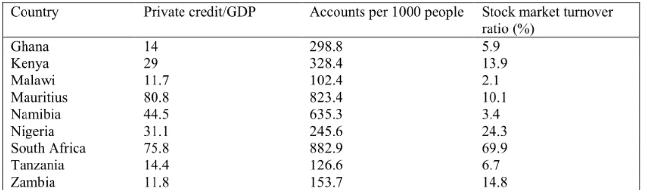
Financial intermediation, process performed by banks of taking in funds from a depositor and then lending them out to a borrower, remains low in Southern regions. This is reflective of the low bank efficiency in the region. As can be seen in Table 1, financial intermediation (as measured by the ratio of private sector credit to GDP) is higher in upper middle-income countries, notably South Africa and Mauritius, but less in low-income countries (Malawi, Uganda, and Tanzania) and those that recently graduated into middle-income status, such as Zambia.
Table 1: Characteristics of financial systems in selected Southern African countries 2008-2012
Country Private credit/GDP Accounts per 1000 people Stock market turnover
ratio (%) Ghana 14 298.8 5.9 Kenya 29 328.4 13.9 Malawi 11.7 102.4 2.1 Mauritius 80.8 823.4 10.1 Namibia 44.5 635.3 3.4 Nigeria 31.1 245.6 24.3 South Africa 75.8 882.9 69.9 Tanzania 14.4 126.6 6.7 Zambia 11.8 153.7 14.8
Table 2: Financial access and outreach in selected Southern African countries, 2012
Country Borrowers from
commercial banks (per 1000 adults) Commercial bank branches (per 1000 adults) Interest rate spread (lending rate-deposit rate) Risk premium on lending Angola - 11.4 13.1 12.7 Botswana 212 8.6 7.4 - Malawi 17 3.3 21.3 16.5 Mauritius - 21.6 2.4 5.6 Mozambique 31 3.8 5.4 11.2 South Africa - 10.4 3.3 3.4 Tanzania 28 2.2 5.9 3.5 Zambia 19 4.4 5.1 -1.9
Source: World Development Indicators
Most of the countries in the region also suffer from low levels of financial penetration or outreach. For instance in Zambia only a third of the adult population has access to a bank account. Further, as Table 1 illustrates, the severity of financial exclusion is mostly manifested in the low number of bank accounts per 1,000 people. This illustrates that there aren’t enough financial institutions willing or ready to carter for all classes in the economy. It can also be the result of the lack of transparency in the economies.
3.
Literature Review
There have been two main approaches for determining the level of competition in the banking sector. These include structural and non-structural tests which both consider the relevant characteristics of banks. One structural approach includes the structure-conduct performance (SCP), while the non-structural approaches have been promoted within the New Empirical Industrial Organisation (NEIO). This section will analyse the evolution of these approaches starting with the theory presented by the SCP and the arguments of the modern approaches. It will conclude with an empirical analysis of the studies in this field of research.
3.1 Theoretical literature
The Structure-Conduct-Performance model (SCP) defined as the relationship between market structure, firm conduct and firm performance suggests that the existence of entry barriers is the major determinant of firm profits, thus the greater cost of entry makes it easier for existing monopolistic firms to maintain profits. According to microeconomic theory, the structure of
the market influences the conduct and behaviour of firms (Sinkey, 1986). The term structure,
in the framework of SCP model, refers to the number of banks serving in the entire industry. Market structure depends on various factors such as competition, regulation as well as
market. This can include pricing, marketing and innovative behaviours of the business of
banking. Lastly, performance refers to the quantity and quality of products and services
provided by the banks in the industry, which determine the profit levels.
SCP model assumes that market structures identified by many firms providing the same products and services, though relatively equal in firm size, are competitive markets generating greater performance. Then, the degree of concentration of banks’ output in a market affects the extent of competition among these banks. The extent of competition affects the price that consumers pay for banking services, which determines the level of profits and performance. The SCP framework suggests that higher concentration leads to higher prices, which in turn lead to higher profits. According to Bain (1951) traditional market SCP claims that market structure influences conduct (behaviour) of firms through pricing policies, and this in turn influences firm performance. The relationship between profitability and market structure has generated competing hypotheses. There are theoretical criticisms to the SCP framework suggested by Demsetz (1973) and later by Berger (1995). These critics believe that the larger market shares, which lead to a higher level of concentration, may be as a result of better efficiency and lower costs rather than a low level of competition. Others (Mullineux & Sinclair, 2000) argue that concentration may lead to higher prices and as a result lower demand, however, it does not mean that a highly concentrated banking sector will have higher profits.
It is for this reason that the new approaches (NEIO) were introduced to measure competition and the view is that both industry structure and performance are determined by other factors; so the approach tests competition and the use of market power but does not assume a causal relationship between market structure and performance (Bikker & Haaf, 2002; Bresnahan, 1989). The Bresnahan and Panzar-Rosse as well as the Lerner-Index and the PE indicator, fall into this part of the literature. The most commonly used structural models are the Panzar and Rosse (Rosse & Panzar, 1987) and the Bresnahan approaches (Bresnahan, 1982). Models specify that how banks behave depend on the market structures in which they operate. Unlike structural methods they do not ignore the relationship between market contestability and revenue behavior at the firm level.
Lately it has been argued that conventional measures of competition like the Lerner- Index and the Panzar-Rosse H-statistic may not assess bank competition in certain economies correctly. The argument is that certain financial rules like the existence of interest rate regulations influence the outcome of these approaches. Instead the relatively new Profit
Elasticity (PE) indicator may be better suited to investigate competitive conditions given any characteristics of the banking industries. This indicator, whose theoretical base is the Relative Profit Differences (RPD) concept, is based on the idea that competition rewards efficiency (Boone et al., 2007; Boone, 2008). The PE indicator will be stronger the more competitive the market is.
3.2 Empirical literature
Although there has been theoretical criticism of the SCP model, several studies (Berger & Hannan, 1989; Neumark & Sharpe, 1992 and Okeahalam, 1998) support the framework. Okeahalam (2001), by analysing the concentration in the industry, attempts to measure the level of competition in the South African banking sector, hence, explore whether or not the current industrial structure of the sector has an impact on the pricing of retail banking deposit products. The investigation followed the SCP framework and concludes that the South African banking sector is highly concentrated. This normally leads to a high likelihood that there will be a collusive oligopoly in the industry. The findings are used to discuss whether this influences the behaviour of banks in credit extension to the currently excluded market sector, the impact it has on the aggregate social welfare function and possible policy implications. Falkena et al. (2004) is another study of the concentration in the South African banking sector, which was carried out as part of a Task Group Report for The National Treasury and the South African Reserve Bank. The study used the Herfindahl-Hirschman Index to determine the concentration in the financial sector. They found that the South African banking sector was in fact highly concentrated, however, based on Falkena et al. (2004) findings the high costs and lack of access to banking services for small and micro-enterprises may have more to do with a number of structural factors than the level of competition in banking. It was difficult to identify studies extending the SCP approach to the Southern region; making it safe to conclude that there is a lack of this sort of literature in those regions. This paper aims to increase the availability of literature for SADC studies. Several studies have attempted testing for competition in the banking sector by the modern approaches. Using a sample of US banking data for the period 1979, Shaffer (1982) identifies a monopolistic competitive banking behaviour in the US. Other earlier applications of the model are in respect of Canadian banks (Nathan & Neave, 1989) and European banks (Molyneux et al., 1994). Nathan & Neave (1989) find monopolistic competition in the Canadian banking sector for the period 1983 and 1984 but perfect competition in the period 1982. Using a sample of European countries over the period 1986 to 1989, Molyneux et al.
(1994) find that banks in France, Germany, Spain and the United Kingdom (UK) behave as though operating under monopolistic competitive conditions whilst those in Italy are classed as though operating under monopoly or conjectural variation short-run oligopoly conditions. Greenberg and Simbanegavi (2009) use both the Panzar-Rosse and the Bresnahan to test for the level of competition in the South African bank sector taking into account that banks behave differently depending on the market in which they operate. They arrive at the conclusion that the sector faces a high level of monopolistic competition. Using the Lerner-Index, Gaertner and Sanya (2012) find that the degree of competition in the East African Community is low due to a combination of structural and socio-economic factors. The analysis ranks the countries in terms of banking sector competitiveness in the following order: Kenya, Tanzania, Uganda and Rwanda.
To explore both time series and cross-sectional variations, applications of the Panzar-Rosse model employ a panel data estimation approach. Studies taking this approach include Al- Muharrami et al. (2006) for the Arab Gulf Cooperation Council’s (GCC) banking system; Bikker & Haaf (2002) for 23 European Union and non-European Union countries and De Bandt & Davis (2000) for a sample of French, German, Italian and US banks. The results of the above studies are generally consistent with monopolistic competition with the exception of a few submarkets.
A recent change in the study of banking competition has been the shift towards regionally classified markets. The reasons behind such a classification include similarity of banking market features. Based on the similarities of characteristics within South Eastern European countries, Mamatzakis et al. (2005) class these countries’ banking sectors as a single banking market and estimate Panzar-Rosse H-statistic for the entire region over the period 1998 to 2002. Depending on the choice of dependent variable, different H-statistics are documented. Moreover, following the introduction of the single Banking Licence in the European Union (EU), Casu & Girardone (2006) apply the Panzar-Rosse model to the study of 15 major European countries’ banking sectors, assuming a common banking market. Their results show that, between the period 1997 and 2003, EU banks behaved as though operating under monopolistic competition. They find H-statistics of 0.362 and 0.364, based on the model specification. In a similar fashion, Fosu (2013) using a dynamic version of the Panzar-Rosse to assess the overall extent of banking competition in each sub-regional banking market over the period 2002 to 2009 conclude that African banks generally demonstrate monopolistic competitive behaviour.
that there are not enough studies, of the other modern approaches, in the literature. This paper takes a different approach in that it will present three results on the extent of bank competition in the SADC region using different modern approaches. The view is that increased regional integration together with advances in information technology and the banking sector reforms mentioned earlier justify the assumption of single banking markets within the Southern African regions.
4.
Data
The data used is bank data from all the registered locally controlled and foreign controlled banks in each of the SADC countries. For both the Panzar-Rosse and the Lerner Index annual data for the period 2002-2013 was used. In the analysis we focus on consolidated data from commercial and savings banks as well as bank holding companies. Excluded are real-estate and mortgage banks, investment banks, other non-banking credit institutions and specialized governmental credit institutions.
Data availability determined which countries were included in the study; although it would have been beneficial to have all the countries’ data it is understandable that data restrictions in the region limited this. The data was obtained from various sources providing information and data on banks across the continent. These include Bankscope and the financial reports obtained directly from the various banks’ websites. This data was fairly feasible; although, this research acknowledged that certain countries would not have all the data required to carry out the study; in that case the respective countries were excluded from the study. The study excluded any banks or periods with missing, negative values or zero values from inputs and
outputs and other relevant data. This sample was restricted to banks with five or more
observations for each country, which is enough to observe significant changes. This did not
have any major drawbacks on the reliability of the study. Also the study uses either the consolidated or the unconsolidated statements depending on which one is available.
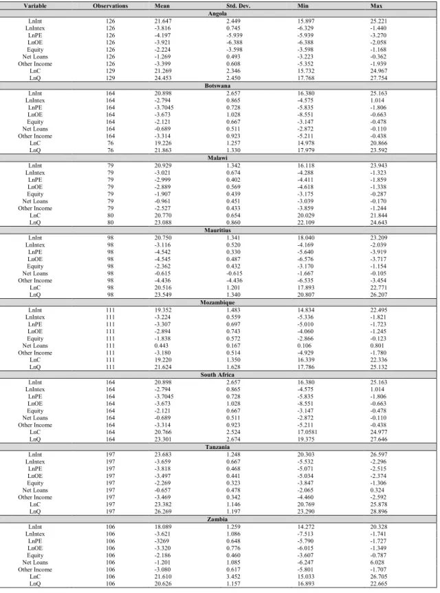
Table A1 in the appendix presents the descriptive statistics of the main variables used in both tests in the study.
5.
Methodology
5.1 Panzar-Rosse Approach
The Panzar-Rosse model, popularised by Rosse & Panzar (1977) and Panzar & Rosse (1987), is an approach to measuring competition that is based on a reduced form revenue or price equation. Many published P-R studies estimate a revenue function that includes total assets (or another proxy of bank size) as a control variable. Other articles estimate a price function instead of a revenue equation, in which the dependent variable is total revenue divided by total assets. For the purpose of this study the revenue equation will be used. Also, different banks will earn more revenue in ways unrelated to variations in input prices so bank specific control variables are added to the model.
From this revenue equation, a measure of competition, H-statistic, is obtained by summing the elasticities of revenue with respect to input prices. The H-statistic measures the degree of competition as the extent to which a change in factor input prices is reflected in revenues earned by a specific bank in equilibrium. Under perfect competition, an increase in input prices raises both marginal costs and total revenues by the same amount as the rise in costs. Under a monopoly, an increase in input prices will increase marginal costs, reduce equilibrium output and consequently reduce total revenues. The H-statistic is estimated from a reduced form bank revenue equation as the sum of the elasticity of the total revenue of the banks with respect to the bank’s input prices. The H-statistic varies between 0 and 1, with the following interpretation;
Because elasticities are required to obtain the H-statistic, the following reduced form log-linear revenue equation is used. This is a variation of the Panzar and Rosse (1987) methodology:
𝐿𝑛(𝐼𝑁𝑇it) = 𝛼 + 𝛽1ln(W1,it) +𝛽2ln(W2,it) + 𝛽3ln(W3,it) + 𝛾1ln(Z1,it) + eit
where i denotes banks and t denotes years. Empirical banking literature often takes interest
income as revenues to capture only the intermediation activities of banks (e.g. Bikker and Haaf, 2002). Similarly, INT is total interest revenue (proxy for banks’ output price), W1 is the ratio of interest expenses to total deposits and money market funding (proxy for input price of
deposits), W2 is the ratio of personnel expenses to total assets (proxy for input price of labour)
and W3 is the ratio of other operating and administrative expenses to total assets (proxy for
input price of equipment/fixed capital). Z is a matrix of controls including the ratio of equity
to total assets, the ratio of net loans to total assets, and the logarithm of assets. These two control variables account for the differences in risks, costs and structure of the individual banks.1 Total Assets will not be included as a proxy for size. According to Bikker et al (2009)
only the unscaled revenue equation yields a valid measure for competitive conduct.
However, the appropriate Panzar-Rosse test, based on an unscaled revenue equation, generally requires additional information about costs and market equilibrium to allow meaningful interpretations.
Finally, αi denote bank-level fixed effects. The H-statistic equals 𝛽1 +𝛽2 + 𝛽3. 5.2 Lerner Index
The Lerner index of market power captures pricing power by measuring a bank’s ability to set price above its marginal cost. It is defined as the difference between banking output prices and marginal costs (“MC”) all relative to prices. In a perfectly competitive system, the price a bank charges for its services should be equal to its MC and therefore, such a bank will have no market power. The greater the deviation, the less competitive the banking system is interpreted to be. By construction, the index ranges from a high of 1 to a low of 0, with higher numbers implying greater market power. The Lerner index is calculated as:
Lernerit =(Pit - MCit)/Pit
The subscript i denotes bank i and the subscript t denotes year t. Price Pit is the ratio of total
revenues (interest and noninterest income) to total assets for bank i at time t, and MCit is the
marginal cost for bank i at time t.
The marginal cost will be derived, in order to extract the elasticity of total cost to the price of the bank’s main inputs. Taking the derivative with respect to total assets from the following translog cost function derives the marginal cost:
lnCit = ∝0i + 𝛽0lnQit + 𝛽0 0.5[lnQit ]2 + ∝1lnW1it + ∝2lnW2it + ∝3lnW3it +𝛽2l lnQit*lnW1it +
𝛽3lnQ1it *lnW2it + 𝛽4lnQit*lnW3it + ∝4lnW1it *lnW2it + ∝5 lnW1it *lnW3it + ∝6lnW2it *lnW3it +
1Due to the unavailability of data within the Africa region these are the only two control variables used
∝7 0.5 [lnW1it]2 + ∝80.5 [lnW2it]2 + ∝90.5 [lnW3it]2 + ∝10ln(Equity)it + ∝11ln(Net Loans)it + F
+ Y + e
The variables in the above equation are defined in table A2.
Assuming that the slope of the cost function within a country is constant through time, the MC for all banks in the study is calculated from the translog cost function regression over the data range. Using the estimated coefficients from the translog cost regression the MC is calculated as follows:
MCit = ( 𝛽0 + 𝛽1* lnQit +𝛽2*lnW1it + 𝛽3*lnW2it +𝛽4*lnW3it ) * (Cit /Total assets)
This equation implies that variations Q, W1, W2, W3, C, total assets and P result in variations
in bank-level Lerner for each country.
6.
Empirical results
6.1 Panzar-Rosse
The revenue equation is estimated using the bank specific fixed effects (“FE”) regressions and the feasible generalised least squares (“FGLS”) method. The study uses the FE within-group estimator technique to account for the heterogeneity amongst the different banks. Given that the technique eliminates the heterogeneity by differencing the sample observations around their sample means, there is no need to use the dummy variable method (Gujarati & Porter, 2009). FGLS is used, as time series data is likely to exhibit autocorrelation and heteroskedasticity problems. The OLS models for each country were tested for serial correlation and the results support the theory that in our time series data the residuals are correlated with each other.
Given that the variables used in the unscaled revenue equations are ratios of total assets, two regressions were ran for the FGLS approach; a scaled variable regression and an unscaled variable regression (correcting the variables to prevent distortions). This is done by replacing all the explanatory variables which are a ratio of total assets, and which have a correlation
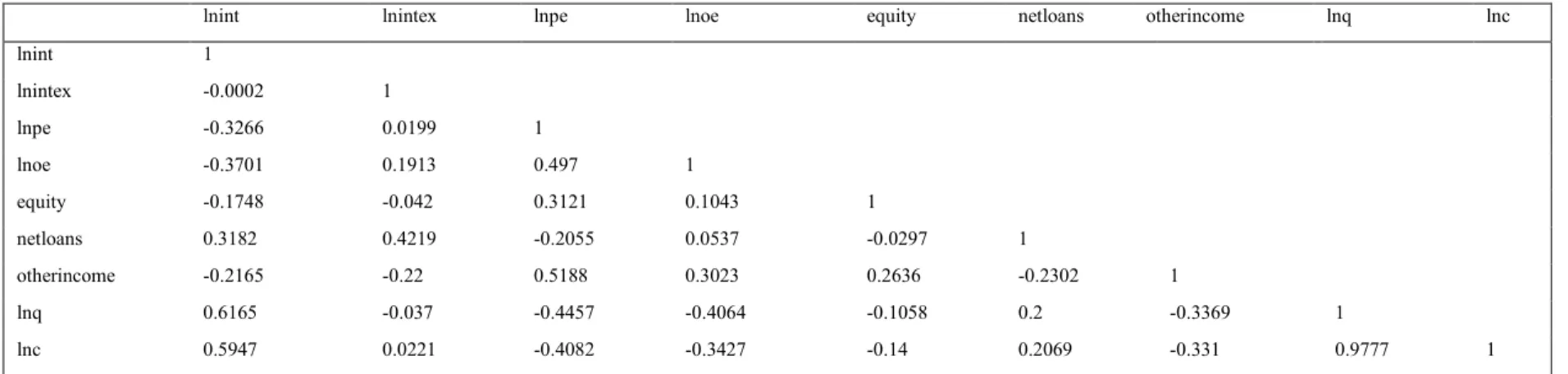
coefficient higher than 0.482, with the residual values. Table A3 was used for the analysis of
correlation among the varibales. For each country the H-statistic is obtained by taking the average of both the FE and the FGLS regressions.
2This is the correlation coefficient cut-off value as used in Bikker et al (2012) and followed in Gwatidzo et
Reported below are the regression outputs of both the FE and the FGLS approaches for each country (See table 4 and table 5). On average the H-statistics based on the within estimator are not very different from the FGLS statistics with the exception of Malawi, Mauritius and Tanzania. Malawi has the biggest difference, which could be the result of the scaling. For the a priori expectations of the regression results refer to table 6 in the appendix. The critical values, which were used to determine the significance of the t-statistics of the Panzar-Rosse test, are presented in table A5.
Angola
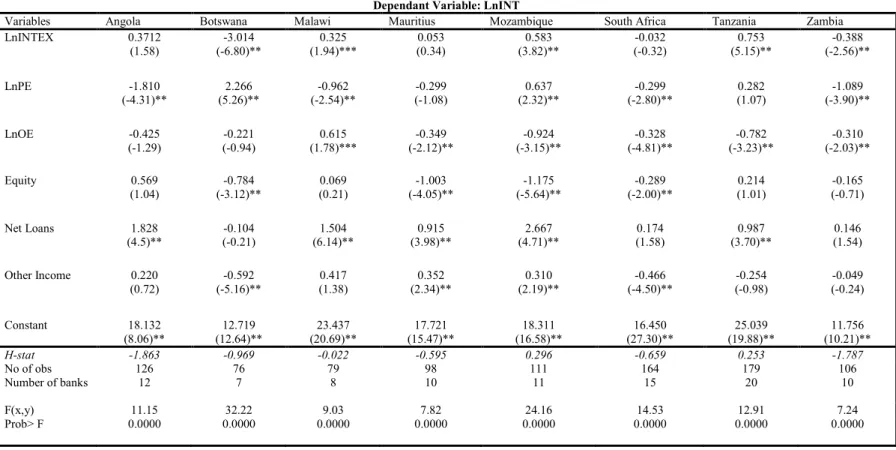
Based on the fixed effects estimation the coefficient on the input price of deposits (LnINTEX) is positive (0.3712) but insignificant. An increase in LnINTEX should result in in a reduction in interest revenue as fewer people make use of the service. Like in any market when a service becomes expensive the consumer will move away from it. The input price of labour (LnPE) is negative at -1.810 and significant at the 5% level. Lastly the input price of fixed capital (LnOE) is negative (-0.425) and significant. The signs of the input prices depend on
the competitive environment in which the banks are operating. This implies that the signs
might differ for the respective banks. All the control variables appear to be positive with only net loans to assets being significant at the 5% level. The sign of loans to total assets (Net Loans) is in line with theory as it is expected to be positive for the revenue equation. Table A5 represents the a priori signs of coefficients in the Panzar-Rosse regressions. Banks compensate themselves for credit risk by means of an additional charge to the lending rate, which then increases its interest income (Bikker et al, 2012). As a result the ratio of equity to total assets is expected to have a negative impact on interest income. This is not the case, however the coefficient for this is insignificant. Summing the three main variables yields an H-statistic= -1.863 rejecting the two null hypotheses that H is statistically different from zero and unity (see table 4).
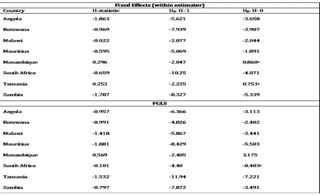
Table 3: Panzer-Rosse H-statistics
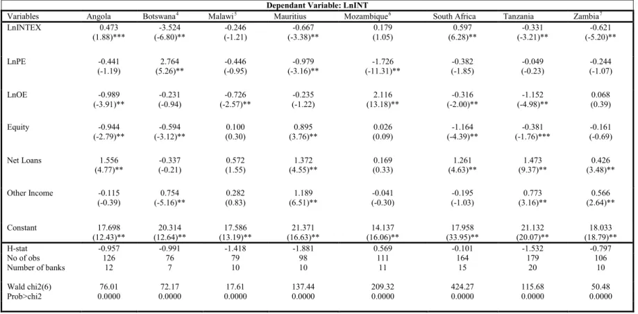
Table 5 displays the results for the FGLS approach. Using the panel FGLS estimation the signs of the input prices of deposits, labour and fixed capital remain the same at 0.473, -0.441, -0.989 respectively. LnPE yields insignificant results. Both equity and loans have the correct signs according to theory and are both significant at the 5% level. An increase in other income will increase interest revenue however its coefficient is insignificant. The H-statistic = -0.957 which is also statistically different from zero and unity.
Averaging the two we get an H-stat= -1.41 which implies that banks in Angola behave like
monopolies. This is the result of many banks being unable to offer sufficient banking services and at reasonable costs.
Botswana, Malawi and Mauritius
Botswana fixed effects estimation coefficient on the LnINTEX is negative (-3.014) and significant; LnPE (2.266) is positive and significant at the 5% level while the LnOE is negative (-0.221). Its control variables appear to be negative with only equity and other income being significant at the 5% level. Equity has the correct sign according to theory. The ratio of equity to total assets is expected to have a negative impact on interest income. Summing the three main variables yields an H-statistic= -0.969 rejecting the two null hypotheses that H is statistically different from zero and unity.
Using the panel FGLS estimation LnPE and LnOE yield contradicting results to what theory suggests. The H-statistic = -0.957 is statistically significant from zero and unity.
Averaging the two we get an H-stat= -0.98which implies that banks in Botswana behave like
monopolies.
Malawi and Mauritius produce the same signs for the FGLS estimation. The coefficients on LnINTEX, LnPE, and LnOE are negative. The control variables are positive with all three
being significant at the 5% level. The average H-statistics are -0.72 and -2.476 for Malawi
and Mauritius respectively. Rejecting the two null hypotheses that H is statistically different from zero and unity.
Averaging the two we get an H-stat= -0.72 which implies that banks in Malawi behave like monopolies. This is the result of many banks being unable to offer sufficient banking services and at reasonable costs.
The sample size for these three countries in particular was very small given the data constraints in a lot of the African countries; this can explain the deviation from theory.
Mozambique and Zambia
Based on the fixed effects estimation the coefficient on LnINTEX is positive and significant for Mozambique (0.583) while Zambia carries a negative a sign (-0.388); LnPE is positive for Mozambique and negative for Zambia. Both of these statistics are significant at the 5% level. Lastly, LnOE is negative for both Mozambique and Zambia (-0.924 and -0.310 respectively). All the control variables appear to be positive with only other income for Zambia being negative but insignificant. The signs of net loans to total assets is in line with theory as it is expected to be positive for the revenue equation. Equity has the correct sign for both countries, which is negative. Summing the three main variables yields the following H=0.296 and H= -1.787 for Mozambique and Zambia respectively, rejecting the two null hypotheses that H is statistically different from zero and unity for Zambia. For Mozambique we fail to reject the null hypothesis that H is statistically different from zero. This suggests that data may not fully support the argument that banks in Mozambique behave in a monopolistically competitive manner.
Using the panel FGLS estimation the signs on LnINTEX, LnPE and LnOE differ slightly from the FE results for Mozambique but not for Zambia. Both equity and loans have the correct signs, for Zambia, according to theory and are both significant at the 5% level. The
H-statistics = 0.569 and -0.797 which is also statistically different from zero and unity. Thus, for Mozambique, competition coexists with high levels of banking market concentration, suggesting contestable market behaviour.
Averaging the two we get H-stat= 0.432 and -1.292 for Mozambique and Zambia
respectively. This implies that banks in Mozambique monopolistically competitive while those in Zambia behave like monopolies.
South Africa and Tanzania
For the two largest countries in the study (in terms of number of banks and financial systems) the fixed effects estimations of LnINTEX is positive and significant for Tanzania (0.753) and negative (-0.032) but insignificant for South Africa. Higher wages lead to a decrease in interest revenue for South Africa and an increase in revenue for Tanzania. The coefficient for South Africa is aligned with theory; hence it is significant at the 5% level while that of Tanzania is insignificant. Two of the control variables have the same signs, positive net loans (which supports theory) and negative other income. The signs on equity are negative for South Africa and positive for Tanzania. How equity impacts revenue is most likely dependent of how these banks use it to generate revenue. Equity being used to innovatively transform the efficiency of a bank can result in higher interest, which is the case for Tanzania. This indicates that lower leverage reduces interest income for SA and increases it for Tanzania. The three main variables yield the following H-statistics, H=-0.659 for SA (rejecting the two null hypotheses that H is statistically different from zero and unity). For Tanzania H= 0.253, where null hypothesis that H is different from zero cannot be rejected.
Using the panel FGLS estimation the signs of LnINTEX switch for the two countries. South Africa has the following values for LnINTEX, LnPE and LnOE; 0.597, -0.382, -0.316 respectively. For Tanzania the same variables are -0.331, -0.049, -1.152 respectively. Both equity and loans have the correct signs according to theory and are both significant at the 5% level. SA H-statistic = -0.101 which is statistically not different from zero. H-statistic for Tanzania= -1.532 and is statically different from zero and unity. It’s unusual to obtain negative H-statistics for South Africa and Tanzania as most studies have found a positive statistic. Testing for competition in the South African banking sector for the periods 1998-2008, Greenberg et al (2013) find a H-statistic of 0.69 while Bikker et al. (2012) arrive at an estimate of 0.410. Gaertner and Sanya (2012) find a statistic of 0.56 for Tanzania after testing for bank competition in the East African Community.
Averaging the two we get an H-stat= -0.38 and -0.639 for SA and Tanzania respectively which implies that banks in both these countries behave like monopolies.
Table 4: Panzar Rosse H-statistic using panel fixed effects estimation3
Parentheses denote the t-statistic as represented in the FE estimation where (*, **, ***) is the significance level at the 1%, 5% and 10% levels respectively.
Dependant Variable: LnINT
Variables Angola Botswana Malawi Mauritius Mozambique South Africa Tanzania Zambia
LnINTEX 0.3712 (1.58) (-6.80)** -3.014 (1.94)*** 0.325 (0.34) 0.053 (3.82)** 0.583 (-0.32) -0.032 (5.15)** 0.753 (-2.56)** -0.388 LnPE -1.810 (-4.31)** (5.26)** 2.266 (-2.54)** -0.962 (-1.08) -0.299 (2.32)** 0.637 (-2.80)** -0.299 (1.07) 0.282 (-3.90)** -1.089 LnOE -0.425 (-1.29) (-0.94) -0.221 (1.78)*** 0.615 (-2.12)** -0.349 (-3.15)** -0.924 (-4.81)** -0.328 (-3.23)** -0.782 (-2.03)** -0.310 Equity 0.569 (1.04) (-3.12)** -0.784 (0.21) 0.069 (-4.05)** -1.003 (-5.64)** -1.175 (-2.00)** -0.289 (1.01) 0.214 (-0.71) -0.165 Net Loans 1.828 (4.5)** (-0.21) -0.104 (6.14)** 1.504 (3.98)** 0.915 (4.71)** 2.667 (1.58) 0.174 (3.70)** 0.987 (1.54) 0.146 Other Income 0.220 (0.72) (-5.16)** -0.592 (1.38) 0.417 (2.34)** 0.352 (2.19)** 0.310 (-4.50)** -0.466 (-0.98) -0.254 (-0.24) -0.049 Constant 18.132 (8.06)** (12.64)** 12.719 (20.69)** 23.437 (15.47)** 17.721 (16.58)** 18.311 (27.30)** 16.450 (19.88)** 25.039 (10.21)** 11.756 H-stat -1.863 -0.969 -0.022 -0.595 0.296 -0.659 0.253 -1.787 No of obs Number of banks 126 12 76 7 79 8 10 98 111 11 164 15 179 20 106 10 F(x,y) 11.15 32.22 9.03 7.82 24.16 14.53 12.91 7.24 Prob> F 0.0000 0.0000 0.0000 0.0000 0.0000 0.0000 0.0000 0.0000
Table 5: Panzar Rosse H-statistic using panel FGLS estimation
4 Equity corrected for scale 5 Net Loans corrected for scale 6 Equity and OE corrected for scale 7 PE corrected for scale
Note: Parentheses denotes the Z-statistic as represented in the FGLS estimation where (*, **, ***) is the significance level at the 1%, 5% and 10% levels respectively.
Dependant Variable: LnINT
Variables Angola Botswana4 Malawi5 Mauritius Mozambique6 South Africa Tanzania Zambia7
LnINTEX 0.473 (1.88)*** (-6.80)** -3.524 (-1.21) -0.246 (-3.38)** -0.667 (1.05) 0.179 (6.28)** 0.597 (-3.21)** -0.331 (-5.20)** -0.621 LnPE -0.441 (-1.19) (5.26)** 2.764 (-0.95) -0.446 (-3.16)** -0.979 (-11.31)** -1.726 (-1.85) -0.382 (-0.23) -0.049 (-1.07) -0.244 LnOE -0.989 (-3.91)** (-0.94) -0.231 (-2.57)** -0.726 (-1.22) -0.235 (13.18)** 2.116 (-2.00)** -0.316 (-4.98)** -1.152 (0.39) 0.068 Equity -0.944 (-2.79)** (-3.12)** -0.594 (0.30) 0.100 (3.76)** 0.895 (0.09) 0.026 (-4.39)** -1.164 (-1.76)*** -0.381 (-0.69) -0.161 Net Loans 1.556 (4.77)** (-0.21) -0.337 (1.55) 0.572 (4.55)** 1.372 (0.33) 0.169 (4.63)** 1.261 (9.37)** 1.473 (3.48)** 0.426 Other Income -0.115 (-0.39) (-5.16)** 0.754 (0.83) 0.282 (6.51)** 1.189 (-0.30) -0.041 (-1.03) -0.195 (3.16)** 0.773 (2.64)** 0.566 Constant 17.698 (12.43)** (12.64)** 20.314 (13.19)** 17.586 (16.63)** 21.371 (16.06)** 14.137 (33.95)** 17.958 (20.07)** 21.132 (18.79)** 18.033 H-stat -0.957 -0.991 -1.418 -1.881 0.569 -0.101 -1.532 -0.797 No of obs Number of banks 126 12 76 7 79 10 10 98 111 11 164 15 179 20 106 10 Wald chi2(6) 76.01 72.17 17.61 137.44 209.32 424.27 115.68 50.48 Prob>chi2 0.0000 0.0000 0.0000 0.0000 0.0000 0.0000 0.0000 0.0000
From the regression outputs the H-statistics for each approach are averaged in order to obtain a single value for each country.
Table 6: Average H-statistics per country
In the recent Banking Enquiry carried out by the Enquiry Panel of the Competition Commission (Jali et al. 2008), it was concluded that the South African banks were not acting as a cartel. Despite this, the panel also believes that the cost and trouble involved for customers to switch banks weakens the competitive effect of price differences between banks. This reduces competition in the market, resulting in certain banks carrying large proportions of the market power in the country.
Given that most of the studies on banking competition (Al-Muharrami et al., 2006 & Bikker et al., 2012) report results that are consistent with monopolistic competition, the findings of this study suggest that recent financial sector reforms and structures in Africa (eg. increase in foreign banks and cooperation between regions) may be affecting the different samples used in each of the studies. Table A6 gives a brief analysis of the banking systems in the eight countries. These characteristics are essential as they affect each country’s results.
As mentioned above, most of the statistics in the sample study yield negative results that contradict past literature. This is the result of many banks being unable to offer sufficient banking services and at reasonable costs. Financial access in Africa is lower than most developing countries. Within each country a few banks already dominate the market, which makes it difficult for smaller and newer bank to gain market power; this causes a lot of banks to struggle to remain operational. This is further aggravated by the introduction of foreign banks into the local markets. In countries like Botswana, where foreign banks dominate the market, it has become almost impossible for the local banks to remain competitive in those challenging environments. However, a negative value may arise under various conditions. In this case more information about costs and the cost curves is generally needed to infer the degree of competition in addition to the correct H-statistic. According to Shaffer (1982b, 1983a) theoretically a profit maximizing equilibrium in which a firm faces a fixed demand
Angola Botswana Malawi Mauritius Mozambique South
Africa Tanzania Zambia
curve with locally constant elasticity and locally linear cost, H can be negative because it equals 1 plus the firm’s perceived elasticity of demand (less than 1). Also if the cost curve is flat at the point where the firm chooses to produce then it is possible to observe a negative H. We can conclude that some of the banks in the countries above are affected by one of these conditions. For the purpose of this study we will assume that one of the two caveats explains the negative H-statistics estimated.
The above findings contradict Fosu (2013) who by using the static Panzar-Rosse model estimated using the panel fixed effect estimation technique. The study indicates how banks in the Southern African region exhibit slight market power compared with the other regions. The H-statistics are positive and statistically significant for all the sub-regional banking markets. North Africa has the highest H-statistic (0.534), followed by West Africa (0.509), East Africa (0.437) and Southern Africa (0.357).
6.2 Lerner Index
This study follows several literatures on the Lerner Index.8 A constrained fixed effects
regression with time dummies is estimated under restrictions of symmetry and homogeneity of degree one in the price of inputs. The study allows for time effects, as it is believed that certain economic factors could have led to changes in the cost function. However, only a year dummy for 2008 will be included to account for the global financial crisis that affected financial sectors across the globe. This two-way effects model was also tested against the fixed effect within-estimator model and for all the countries this model proves to be a better fit. This constitutes our preferred model.9
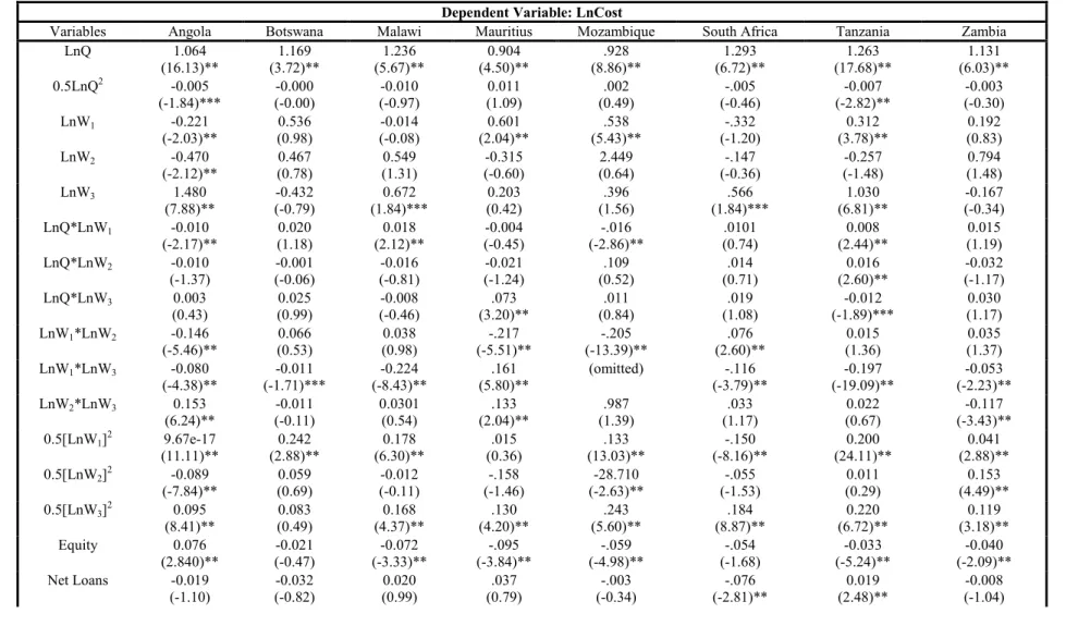
The regression output is presented in table 7 below. Immediately it can be noted that the coefficients for total assets (LnQ) are positive and significant at the 5% level for all the countries in the study. In Angola, Malawi and South Africa the coefficients for the input price of deposits (LnW1) are negative but insignificant, while the rest of the countries have positive estimates. Again Angola and South Africa along with Mauritius and Tanzania have negative signs for the input price of labour (LnW2). This is inconsistent with theory, as an increase in personnel expenses should increase the operation costs to the bank. Looking at the estimates
8There is extensive literature measuring bank competition using the Lerner Index. See Berger, Klapper and
Turk-Ariss (2009), Anzoategui, Peria and Rocha (2010), and Gaertner and Sanya (2012), among others.
9There were some exceptions from countries like Botswana and Malawi, which could be the result of the small
data samples. However, using the two-way effect model for these countries should not have a major impact on the outcome of the analysis.
for other operating expenses (LnW3), only Botswana and Zambia estimates contradict theory. However the negative values are insignificant which imply that there exists a gap between the literature and data. The next variables of interest are the control variables (equity and net loans). Equity is estimate to have a negative and significant coefficient for all the countries excluding Angola. Only Angola, Botswana, Mauritius, South Africa and Zambia have negative signs for net loans while the rest are positive. However, the negative sign on net loans should not be concerning as the loans could be used to condense the banks’ existing costs. In this case an assumption that the benefits of reducing the total costs, using the loan amounts, outweighs the cost incurred on the loan. The estimate on the time dummy that was added to capture the effects of possible structural changes in the banking sectors is satisfactory. The results of all the countries, excluding South Africa and Tanzania, are insignificant which indicate that structural changes did not impact bank operations in these countries. However, given the size of these economies it is unlikely that this was the case. The results could have been skewed by the lack of sufficient data in these countries. As can be seen for South Africa and Tanzania, the 2008 financial crisis seems to have had an impact on bank operations.
Table 7:Lerner Index using the fixed effects10 regression with year dummies
Dependent Variable: LnCost
Variables Angola Botswana Malawi Mauritius Mozambique South Africa Tanzania Zambia
LnQ 1.064 (16.13)** (3.72)** 1.169 (5.67)** 1.236 (4.50)** 0.904 (8.86)** .928 (6.72)** 1.293 (17.68)** 1.263 (6.03)** 1.131 0.5LnQ2 -0.005 (-1.84)*** (-0.00) -0.000 (-0.97) -0.010 (1.09) 0.011 (0.49) .002 (-0.46) -.005 (-2.82)** -0.007 (-0.30) -0.003 LnW1 -0.221 (-2.03)** (0.98) 0.536 (-0.08) -0.014 (2.04)** 0.601 (5.43)** .538 (-1.20) -.332 (3.78)** 0.312 (0.83) 0.192 LnW2 -0.470 (-2.12)** (0.78) 0.467 (1.31) 0.549 (-0.60) -0.315 (0.64) 2.449 (-0.36) -.147 (-1.48) -0.257 (1.48) 0.794 LnW3 1.480 (7.88)** (-0.79) -0.432 (1.84)*** 0.672 (0.42) 0.203 (1.56) .396 (1.84)*** .566 (6.81)** 1.030 (-0.34) -0.167 LnQ*LnW1 -0.010 (-2.17)** (1.18) 0.020 (2.12)** 0.018 (-0.45) -0.004 (-2.86)** -.016 (0.74) .0101 (2.44)** 0.008 (1.19) 0.015 LnQ*LnW2 -0.010 (-1.37) (-0.06) -0.001 (-0.81) -0.016 (-1.24) -0.021 (0.52) .109 (0.71) .014 (2.60)** 0.016 (-1.17) -0.032 LnQ*LnW3 0.003 (0.43) (0.99) 0.025 (-0.46) -0.008 (3.20)** .073 (0.84) .011 (1.08) .019 (-1.89)*** -0.012 (1.17) 0.030 LnW1*LnW2 -0.146 (-5.46)** (0.53) 0.066 (0.98) 0.038 (-5.51)** -.217 (-13.39)** -.205 (2.60)** .076 (1.36) 0.015 (1.37) 0.035 LnW1*LnW3 -0.080 (-4.38)** (-1.71)*** -0.011 (-8.43)** -0.224 (5.80)** .161 (omitted) (-3.79)** -.116 (-19.09)** -0.197 (-2.23)** -0.053 LnW2*LnW3 0.153 (6.24)** (-0.11) -0.011 0.0301 (0.54) (2.04)** .133 (1.39) .987 (1.17) .033 (0.67) 0.022 (-3.43)** -0.117 0.5[LnW1]2 9.67e-17 (11.11)** (2.88)** 0.242 (6.30)** 0.178 (0.36) .015 (13.03)** .133 (-8.16)** -.150 (24.11)** 0.200 (2.88)** 0.041 0.5[LnW2]2 -0.089 (-7.84)** (0.69) 0.059 (-0.11) -0.012 (-1.46) -.158 (-2.63)** -28.710 (-1.53) -.055 (0.29) 0.011 (4.49)** 0.153 0.5[LnW3]2 0.095 (8.41)** (0.49) 0.083 (4.37)** 0.168 (4.20)** .130 (5.60)** .243 (8.87)** .184 (6.72)** 0.220 (3.18)** 0.119 Equity 0.076 (2.840)** (-0.47) -0.021 (-3.33)** -0.072 (-3.84)** -.095 (-4.98)** -.059 (-1.68) -.054 (-5.24)** -0.033 (-2.09)** -0.040 Net Loans -0.019 (-1.10) (-0.82) -0.032 (0.99) 0.020 (0.79) .037 (-0.34) -.003 (-2.81)** -.076 (2.48)** 0.019 (-1.04) -0.008
10 Included in the regression are dummies that represent the bank-specific effects for each bank. Each country contains (N-1) dummies, where N is the number of banks in the sample
T2008 -0.004 (-0.20) 0.0193 (0.81) (-0.68) -0.013 (0.75) .010 (-0.81) -.006 (2.66)** 0.073 (-2.09)** -0.009 -0.005 (0.12) Constant -0.460 (-0.63) (-0.58) -2.167 (-0.95) -2.025 (0.33) .775 (0.89) .972 (-2.17)** -4.317 (-3.11)** -2.970 (-0.87) -1.462 F(x,y) 7548.75 2085.26 2261.49 4080.11 13012.58 4250.15 19352.06 14476 Prob > F 0.0000 0.0000 0.0000 0.0000 0.0000 0.0000 0.0000 0.0000 R2 Number of banks 0.999 12 0.998 7 0.999 8 0.999 10 0.997 11 0.999 15 0.999 20 0.999 10 Lerner Index11 0.524 0.406 0.487 0.367 0.351 0.410 0.460 -0.924
11Lerner Index is calculated as (P-MC/P) where P= total gross revenue of the bank to total assets and MC= marginal cost as calculated using the estimated coefficients (see LI
Using the coefficients of the regression output, the Lerner Index for each country was calculated. The Lerner Index ranges between -9.24 in Zambia and 0.524 in Angola. Figure 1 below illustrates that Angola, Malawi, South Africa and Tanzania have the highest indices (52%, 48.7%, 41% and 46% respectively) of the 8 countries. These countries are the least competitive, which implies that they are not too far from
behaving like monopolies. Clerides et al. (2013) estimated the degree of competition
in the banking sector of 148 countries over the period 2007-2010 estimate the following indices for these four countries; 39.3%, 40.7%, 20.7%, 40.1% respectively. The estimates for Malawi and Tanzania are not too far off (ranging between 40% and 50%) for the two studies. Gaertner and Sanya (2012) find an index of 32% for the period 2001-2008. The differences could be explained by factors such as data selection, sample size, and variables of choice and estimation methods. The indices of the other four countries Botswana, Mauritius, Mozambique and Zambia are 40.6%, 36.7%, 35.1% and -92.4% respectively, not too far away from the top four countries
(with the exception of Zambia). Clerides et al. (2013) estimate 31.2%, 26.6%, 29.6%,
and 23.0% respectively. The mean values for the two studies were calculated and the
following values were found, 26.0% for this study and 31.4% for Clerides et al.
(2013). It is not uncommon for the Lerner Index to take on negative values, the case for Zambia. According to Solis and Maudos (2008), this denotes ‘super competition’ which occurs when banks price below marginal cost-such as the case of initial subsidisation. Musonda (2013), who studies bank competition in Zambia, found that the Lerner Index for the country begins to decline into the negatives post 2008. The paper suggests that this could be the result of new banks trying to gain market share or existing banks trying to emerge from the global financial crisis by reducing prices in order to regain their market share.
Although we find different results, it can be concluded that all 8 countries typically have an insignificant amount of market power suggesting that banks in the SADC region have competitive market systems. Perhaps they can be characterised by a monopolistically competitive system. This is consistent with the above study, which finds that Sub-Saharan African, East-Asian and Pacific banking systems seem to be the least competitive ones.
The above statement can be supported by individually analysing bank performance in each of these countries (see graph A1).
Looking at Angola we can see that prior to 2007 banks such as Banco Sol, and Banco Keve exhibited low market power compared with the other banks. Banco Keve declined drastically from its 2002 position. However this all changed after 2007 where all the banks in the sample have a constant trend around the same average between 0 and 1 for the rest of the period. This is also true for Tanzania, which has a constant trend. In Malawi the LI’s for each bank are also following the same trend with one or two banks standing out above the rest. Majority of the banks in SA only start experiencing gradual increases in the LI’s post the 2005 period. ABSA is the only bank that seems to have experienced a drastic decline between the periods 2002 and 2006.
All the graphs illustrate some type of an increase in market power just before the 2008 mark. This pattern change may reflect the sharp increase in financial globalisation before the financial crisis in 2007/2008 and related reforms and the gradual penetration of foreign banks in the local markets. These are likely to have led to changes in market power through mergers and acquisitions. Also, the graphs below (mainly Angola, Malawi and Tanzania) illustrate that the start of the global financial
crisis coincides with a decrease in the market power. This may be related to capital losses and non-performing loans suffered by many banks and rising costs which increased the cost of lending.
6.3 Robustness Checks
Two approaches of bank competition were estimated and the results of each of these yielded different conclusions. Starting with the Panzar-Rosse approach, the two tests (using the panel fixed effects and the FGLS approach) yield different results in terms of the magnitude. However, the same conclusion can be arrived at as for both tests the statics have the same signs. Tanzania was a special case as it yielded a positive H-statistic for the first test and a negative H-statistic for the second test. Unlike the Lerner Index approach, the Panzar_Rosse was not able to generate the same conclusion as most literature (Bikker et al, 2012; Fosu, 2013). However, the possibility of a monopolistic banking competition in these countries is not impossible. The Lerner Index is consistent with what was suggested by past literature. The conclusion that the SADC countries are slightly far from behaving like monopolies is consistent with
Clerides et al. (2013) and Gaertner and Sanya (2012).
It can be concluded that the two approaches do not generate robust results and hence conclusions. This implies that a solid conclusion cannot be reached regarding the extent of bank competition in the SADC region.
7.
Conclusion
Barriers to banking services do not only include accessibility but also inappropriate pricing and products. However, competition can correct this. Competition in the banking sector is extremely important given the fundamental role that banks play in the accessibility of credit, the implementation of monetary policy and the maintenance of systemic stability. All of these are crucial for economic development and so it is essential for sufficient competition to exist in this sector in order to ensure the smooth and efficient functioning of the banks. Nonetheless very few studies exist on bank competition in the southern African countries-with the exception of South Africa, compared with the vast literature existing for developed regions. Using two approaches, the Panzar-Rosse model and Lerner-Index this paper analyses whether there exists enough competition in the SADC banks to ensure that the region
continues to develop as it has.
The Panzar-Rosse H-statistic shows that most of the banking system in the SADC region can be categorized as monopolies. This implies that there exist formal regulatory barriers to entry. Mozambique is the only country that is categorized as monopolistic competition. Structural impediments exist, that enable some banks in the country to continue to enjoy a degree of monopoly power. This outcome is not consistent with past literature. Broadly speaking, banks in the SADC are less competitive than other countries with a higher level of financial and economic development. However, when using the Lerner Index the results are similar to some
past empirical findings (Clerides et al., 2013). The conclusion reached is that all 8
countries typically have an insignificant amount of market power suggesting that banks in the SADC region have competitive market systems. These countries could possibly be characterised by a monopolistically competitive system.
Studies of this nature can also help governments identify whether certain structural changes are have a negative or positive impact on the major sector of the economy as more reforms are introduced in the financial sector. This study deviates from existing literature, as it will contribute to the insufficient body of knowledge for SADC studies.
8.
Appendix
Table A1: Descriptive Statistics
Table A2: Lerner Index variables
Cit Total operating & financial costs for bank I in time period t
Variable Observations Mean Std. Dev. Min Max
Angola LnInt 126 21.647 2.449 15.897 25.221 LnIntex 126 -3.816 0.745 -6.329 -1.440 LnPE 126 -4.197 -5.939 -5.939 -3.270 LnOE 126 -3.921 -6.388 -6.388 -2.058 Equity 126 -2.224 -3.598 -3.598 -1.168 Net Loans 126 -1.269 0.493 -3.223 -0.362 Other Income 126 -3.399 0.608 -5.352 -1.939 LnC 129 21.269 2.346 15.732 24.967 LnQ 129 24.453 2.450 17.768 27.754 Botswana LnInt 164 20.898 2.657 16.380 25.163 LnIntex 164 -2.794 0.865 -4.575 1.014 LnPE 164 -3.7045 0.728 -5.835 -1.806 LnOE 164 -3.673 1.028 -8.551 -0.663 Equity 164 -2.121 0.667 -3.147 -0.478 Net Loans 164 -0.689 0.511 -2.872 -0.110 Other Income 164 -3.314 0.923 -5.211 -0.438 LnC 76 19.226 1.257 14.978 20.866 LnQ 76 21.863 1.330 17.979 23.592 Malawi LnInt 79 20.929 1.342 16.118 23.943 LnIntex 79 -3.021 0.674 -4.288 -1.323 LnPE 79 -2.999 0.402 -4.411 -1.859 LnOE 79 -2.889 0.569 -4.618 -1.338 Equity 79 -1.907 0.439 -3.175 -0.287 Net Loans 79 -0.961 0.451 -3.039 -0.170 Other Income 79 -2.527 0.433 -3.859 -1.244 LnC 80 20.770 0.654 20.029 21.844 LnQ 80 23.088 0.860 22.109 24.643 Mauritius LnInt 98 20.750 1.341 18.040 23.209 LnIntex 98 -3.116 0.520 -4.169 -2.039 LnPE 98 -4.542 0.330 -5.640 -3.919 LnOE 98 -4.545 0.487 -6.576 -3.717 Equity 98 -2.362 0.432 -3.170 -1.154 Net Loans 98 -0.615 -0.615 -1.667 -0.105 Other Income 98 -4.436 -4.436 -6.535 -3.454 LnC 98 20.516 1.201 17.893 22.771 LnQ 98 23.549 1.340 20.807 26.207 Mozambique LnInt 111 19.352 1.483 14.834 22.495 LnIntex 111 -3.224 0.559 -5.336 -1.821 LnPE 111 -3.307 0.697 -5.010 -1.723 LnOE 111 -2.894 0.743 -4.060 -1.245 Equity 111 -1.838 0.572 -2.866 -0.123 Net Loans 111 0.443 0.167 0.106 0.801 Other Income 111 -3.180 0.514 -4.929 -1.780 LnC 111 19.220 1.350 16.339 22.336 LnQ 111 21.624 1.628 17.786 25.132 South Africa LnInt 164 20.898 2.657 16.380 25.163 LnIntex 164 -2.794 0.865 -4.575 1.014 LnPE 164 -3.7045 0.728 -5.835 -1.806 LnOE 164 -3.673 1.028 -8.551 -0.663 Equity 164 -2.121 0.667 -3.147 -0.478 Net Loans 164 -0.689 0.511 -2.872 -0.110 Other Income 164 -3.314 0.923 -5.211 -0.438 LnC 164 20.766 2.524 17.0581 24.977 LnQ 164 23.301 2.674 19.375 27.646 Tanzania LnInt 197 23.683 1.248 20.303 26.597 LnIntex 197 -3.659 0.667 -5.532 -2.296 LnPE 197 -3.818 0.468 -5.071 -2.515 LnOE 197 -3.497 0.441 -5.034 -2.374 Equity 197 -2.269 0.323 -3.847 -1.306 Net Loans 197 -0.657 0.478 -2.065 0.324 Other Income 197 -3.469 0.342 -4.460 -2.592 LnC 197 23.382 1.146 20.769 25.878 LnQ 197 26.269 1.197 23.290 28.896 Zambia LnInt 106 18.089 1.259 14.272 20.328 LnIntex 106 -3.621 1.086 -7.513 -1.741 LnPE 106 -3269 0.648 -5.790 -1.727 LnOE 106 -3.320 0.776 -6.015 -1.349 Equity 106 -2.186 0.460 -3.607 -0.787 Net Loans 106 -1.201 1.085 -6.247 6.028 Other Income 106 -3.080 0.617 -5.801 -1.707 LnC 106 21.610 3.452 15.033 26.705 LnQ 106 20.626 1.157 16.893 22.665
Q Total Assets
W1 Interest expenses/ total deposits
W2
Personnel expenses /total assets
W3 Other operating & administrative expenses/total assets
Equity Equity/total assets Net Loans Net loans/total assets
F Firm-specific effects
Y Set of year dummies
Table A3: Correlation Matrices of the main variables Angola:
lnint lnintex lnpe lnoe equity netloans otherincome lnq lnc
lnint 1 lnintex -0.0002 1 lnpe -0.3266 0.0199 1 lnoe -0.3701 0.1913 0.497 1 equity -0.1748 -0.042 0.3121 0.1043 1 netloans 0.3182 0.4219 -0.2055 0.0537 -0.0297 1 otherincome -0.2165 -0.22 0.5188 0.3023 0.2636 -0.2302 1 lnq 0.6165 -0.037 -0.4457 -0.4064 -0.1058 0.2 -0.3369 1 lnc 0.5947 0.0221 -0.4082 -0.3427 -0.14 0.2069 -0.331 0.9777 1 Botswana:
lnint lnintex lnpe lnoe equity netloans otherincome lnc lnq
lnint 1 lnintex -0.1067 1 lnpe 0.0062 0.9583 1 lnoe 0.1314 -0.2723 -0.3171 1 equity -0.4932 -0.4924 -0.5871 0.3091 1 netloans 0.0796 -0.1494 -0.1109 0.3706 0.3154 1 otherincome 0.3756 0.0869 0.1317 0.2136 -0.2401 -0.0977 1 lnc 0.9927 -0.0395 0.0718 0.1085 -0.568 0.023 0.3896 1 lnq 0.9849 -0.211 -0.0845 0.0718 -0.4879 0.0419 0.354 0.9793 1
Malawi:
lnint lnintex lnpe lnoe equity netloans otherincome lnc lnq
lnint 1 lnintex -0.1641 1 lnpe -0.267 0.4025 1 lnoe -0.2995 0.2321 0.5413 1 equity -0.1513 0.0617 0.5013 0.357 1 netloans 0.4696 -0.1307 -0.1683 -0.137 -0.4369 1 otherincome -0.132 -0.063 0.3101 0.4478 0.3059 0.0256 1 lnc 0.6245 -0.0642 -0.3286 -0.1146 -0.0393 0.2312 -0.2017 1 lnq 0.6742 -0.2718 -0.4374 -0.3217 -0.0837 0.3036 -0.2195 0.9248 1 Mauritius:
lnint lnintex lnpe lnoe equity netloans otherincome lnc lnq
lnint 1 lnintex -0.1642 1 lnpe -0.0092 0.2216 1 lnoe -0.1107 0.2085 0.4339 1 equity 0.3364 0.2963 0.2877 -0.098 1 netloans 0.2553 -0.1147 0.0545 0.1587 -0.0286 1 otherincome 0.535 0.0597 0.4886 0.1973 0.382 0.0428 1 lnc 0.9938 -0.109 0.0079 -0.0682 0.3349 0.2387 0.5445 1 lnq 0.9655 -0.3777 -0.0742 -0.2268 0.2801 0.2116 0.4758 0.9528 1 Mozambique:
lnint lnintex lnpe lnoe equity netloans otherincome lnc lnq lnint 1 lnintex 0.0856 1 lnpe -0.2494 0.3088 1 lnoe -0.5103 0.3415 0.847 1 equity -0.7832 -0.0631 0.401 0.5985 1 netloans 0.0891 0.3274 0.0066 0.0807 0.1391 1 otherincome -0.2178 -0.1123 0.2516 0.2335 0.2166 -0.2655 1 lnc 0.9659 0.1025 -0.2187 -0.4407 -0.7797 0.0223 -0.1986 1 lnq 0.9425 -0.1164 -0.4683 -0.7009 -0.8189 -0.0391 -0.2306 0.9418 1 South Africa:
lnint lnintex lnpe lnoe equity netloans otherincome lnc lnq
lnint 1 lnintex 0.2695 1 lnpe -0.4043 0.0455 1 lnoe -0.4855 0.0324 0.6336 1 equity -0.4939 0.1875 0.663 0.6603 1 netloans 0.5331 0.4068 -0.1463 -0.3415 -0.2857 1 otherincome -0.4359 0.1031 0.6795 0.7345 0.7295 -0.3283 1 lnc 0.9809 0.2589 -0.4055 -0.4124 -0.4503 0.489 -0.3396 1 lnq 0.9825 0.1672 -0.4805 -0.5282 -0.5372 0.4916 -0.4424 0.9843 1
Tanzania:
lnint lnintex lnpe lnoe equity netloans otherincome lnc lnq
lnint 1 lnintex -0.2065 1 lnpe 0.0389 0.0611 1 lnoe -0.0173 -0.0401 0.7888 1 equity -0.0771 0.018 -0.311 -0.3228 1 netloans 0.3064 0.0311 0.3772 0.4372 -0.0346 1 otherincome 0.0372 -0.2238 0.4686 0.4813 -0.2522 -0.077 1 lnc 0.9751 -0.1222 0.1321 0.1201 -0.1304 0.3471 0.079 1 lnq 0.974 -0.3242 -0.0763 -0.1079 -0.044 0.2163 0.0214 0.9479 1 Zambia:
lnint lnintex lnpe lnoe equity netloans otherincome lnc lnq
lnint 1 lnintex -0.2136 1 lnpe -0.0476 0.6269 1 lnoe 0.0418 0.509 0.6161 1 equity -0.1592 0.2122 0.213 0.1432 1 netloans 0.267 0.402 0.3994 0.3876 0.0372 1 otherincome 0.1981 0.5271 0.5367 0.4323 -0.0075 0.4375 1 lnc 0.0565 -0.1495 -0.2729 -0.0252 0.0145 -0.0895 -0.1465 1 lnq 0.9129 -0.5131 -0.3095 -0.1694 -0.2429 0.0885 -0.0273 0.1806 1
Table A4: Critical values for the test of significance
Reject at 1% level Reject at 5% level Reject at 10% level Angola, Mauritius,
Mozambique 2.617 1.980 1.658
Botswana, Malawi, Zambia 2.66 2.00 1.671
Tanzania, South Africa 2.576 1.960 1.645
Table A5: Expected signs for the Panzar-Rosse model
Variables Bikker et al. (2012) Description
LnINTEX +/- The sign of input prices in the revenue equation
will depend on the competitive environment (perfect/imperfect competition)
LnPE LnOE
Equity - Lower equity ratio mplies more leverage and
hence more interest income
Net Loans + Banks compensate themselves for credit risk by
means of an extra fee on the lending rate, which increases interest income
Other Income - As banks increase their share of non-interest
earning assets interest income decreases
Table A6: Structure and analysis of the banking systems in the SADC regions
Angola:
Angola’s financial system is highly concentrated. The top five banks account for 77% of total assets. Although banking coverage expanded from 22% in 2010 to 51% in 2013, it is still concentrated in Luanda. There are 22 commercial banks in Angola with six banks in the ranking of the top 100 largest banks on the African continent (African Business Magazine)
Botswana:
Botswana’s financial sector is small and dominated (by asset size) by commercial banks and pension funds. With only 10 commercial banks in Botswana of which three are listed on the stock exchange, it has resulted in the cost of borrowing, including interest rates and other types of charges being relatively high in the country.
Malawi:
Banks are dominant in Malawi’s financial system accounting about 80% of total financial sector assets. Two banks hold slightly more than half of the banking industry’s total assets and deposits. Only 19% of the population have access to financial services. Access to finance is a major challenge, especially for SMEs. Malawi is currently transitioning to Basel II accords, which will require banks to raise more capital.
Mauritius:
Banks are well capitalised, with 15% of Regulatory Tier I capital to risk-weighted assets well above the proposed Basel III requirements. Mauritius has 23 commercial banks with about 10 largest banks in Africa. Large foreign banks are also present in Mauritius. Most commercial banks diversified into non-banking business through subsidiaries and affiliates. There are 11 commercial banks in Malawi.
Mozambique:
There are 18 registered commercial banks in Mozambique representing 95% of total financial system assets. However, 85% of the financial sector’s assets are concentrated in the three largest banks, all of which are foreign owned (two Portuguese and a South African).
South Africa:
In 2013 the banking sector accounted for R3.8 trillion. The rapid expansion of non-secured lending to households, which currently accounts for about 12% of total banking exposure, has increased credit risk. Domestic banks are capitalised above the new Basel III levels and are currently operating above the minimum requirement. The country has over 50 banks of locally-controlled commercial banks, foreign-controlled ones, branches of foreign banks, foreign bank representatives, mutual banks and others.