Incorporating innovation subsidies
in the CDM framework:
Empirical evidence from Belgium
Dirk Czarnitzki and Julie Delanote
Incorporating innovation subsidies in the CDM
framework: empirical evidence from Belgium
— forthcoming inThe Economics of Innovation and New Technology— Dirk Czarnitzkiaand Julie Delanoteb
a) KU Leuven, Dept. of Managerial Economics, Strategy and Innovation, Belgium; Center for R&D Monitoring (ECOOM) at KU Leuven, and ZEW Mannheim, Germany
b) KU Leuven, Dept. of Managerial Economics, Strategy and Innovation, Belgium, and Center for R&D Monitoring (ECOOM) at KU Leuven, Belgium
This version: May 2016
Abstract
This paper integrates innovation input and output effects of R&D subsidies into a modified Crépon–Duguet–Mairesse (CDM) model. Our results largely confirm insights of the input ad-ditionality literature, i.e. public subsidies complement private R&D investment. In addition, results point to positive output effects of both purely privately funded and subsidy–induced R&D. Furthermore, we do not find evidence of a premium or discount of subsidy–induced R&D in terms of its marginal contribution on new product sales when compared to purely privately financed R&D.
Keywords:CDM model, R&D, subsidies, innovation policy
JEL–Classification:C14, C30, O38
Contact details:
Dirk Czarnitzki, KU Leuven, Faculty of Business and Economics Naamsestraat 69
3000 Leuven, Belgium
E-Mail: [email protected]
Julie Delanote, KU Leuven, Faculty of Business and Economics Naamsestraat 69
3000 Leuven, Belgium
1
Introduction
The beneficial effect of business R&D efforts on technological change and growth has been widely acknowledged by scholars and policy makers (Romer, 1990; Mansfield, 1988, 1962; Aghion and Howitt, 1998; Scherer, 1965; Geroski and Toker, 1996). For this reason, governments in industrialized countries spend considerable amounts of money for supporting R&D activities of firms which is mainly justified by the will to overcome presumed market failures (Nelson, 1959; Arrow, 1962; Stiglitz and Weiss, 1981) that lead to an underinvestment in R&D from a social point of view. One of the main governmental instruments in this context are public R&D grants. Based upon policy and academic interest towards this topic, evaluating the effects of such policy instruments has a long tradition in empirical innovation research (see David et al., 2000; Cerulli, 2010; Zúñiga Vicente et al., 2014 for surveys).
So far, the main focus in the literature has been on input additionality of R&D grants, while only some studies assess their impact on output. Rarely, the interrelated nature of these input and output stages has been accounted for by using a simulta-neous equation model. Consequently, this paper takes a more structural approach in order to integrate both stages into one econometric model. This is done by apply-ing a conceptually new variant of the Crépon–Duguet–Mairesse (CDM) framework (Crépon et al., 1998). The resulting model allows to estimate input and output addi-tionality effects of subsidies and, in particular, whether subsidized projects generate a discount or premium in terms of innovation outcome when compared to the non– subsidized, i.e. purely privately financed, projects.
The remainder of the paper is organized as follows: the next section sketches the framework of this paper, both conceptually and methodologically. The third section presents the econometric model. Data and variables are discussed in section 4 and section 5 discusses the empirical implementation and results before concluding.
2
Background
2.1
Conceptual background
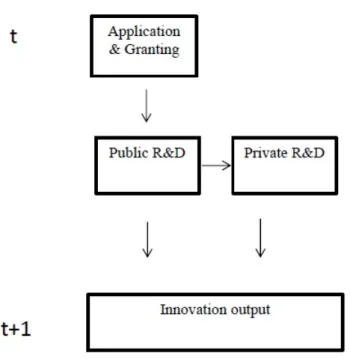
Figure 1 shows a representation of how subsidies may impact the input and output stages of R&D. First, a firm may choose to apply for a R&D subsidy, and the pub-lic agency decides whether or not to grant a subsidy. Furthermore the agency also decides on the subsidy rate, i.e. the share of the total cost of the proposed project that will be covered by the subsidy (see e.g. Takalo et al., 2013 for a structural model on the decision process).1 When learning about the amount of public R&D becom-ing available, the firm will decide on how much to invest in R&D privately. Policy makers hope that subsidizing R&D has a positive effect on the amount firms invest privately. The policy makers logic is intuitive: the firm would not have conducted the project without the subsidy; due to the positive decision on the public R&D grant, however, the firm then conducts the project in addition to others that it would have implemented even in absence of subsidies. As the subsidy never covers the full cost of the proposed R&D project, the government expects that also private R&D increases as response to the R&D grant. As a result, both the public and the private R&D will generate additional innovation output and thus foster technological change in the future. In Figure 1 this is depicted as innovation output in periodt+1.
However, this positive picture on how subsidies help to spur innovation and tech-nological progress may not apply in reality for two reasons. First, the firms might ap-ply with projects that they would even conduct at the same scale if no subsidies were granted. In this case, the subsidy scheme would be subject to so-called full crowding– out effects and no additional R&D projects would be conducted in the economy. In-stead, the granted public funds would simply replace parts of the private investment. Second, even if the subsidized firms implement the subsidized projects in addition to
1The maximum subsidy rate is usually limited to 50% of the total project cost in the EU, but there are exceptions for small and medium–sized firms and for firms in structurally weak regions (so–called Objective 1 regions) where the maximum subsidy rate may exceed 50%.
Figure 1: subsidy-extension of CDM framework
their other R&D activities as expected by the government, and so-called input addi-tionality is thus present, the publicly invested R&D may not necessarily also lead to output additionality, that is, more innovation. As Goolsbee (1998) argues, the granted subsidies might be redirected to higher wages of researchers instead of hiring new staff and/or investing this money in other research–related assets. If higher wages do not coincide with higher marginal productivity of R&D labor, one would find evidence for input additionality but not output additionality. Furthermore, the sub-sidized R&D project might be riskier than the R&D projects that are funded fully privately (see David et al., 2000), and therefore the failure rate might be high, and thus no output additionality may be present either.
Moreover, it is questionable whether the contribution of public R&D to output ad-ditionality at the firm-level is higher or lower than the private marginal productivity. There are reasons for both: given the arguments above on factors that may limit the output additionality of subsidized R&D, it could, on the one hand, be argued that subsidized R&D has a lower marginal productivity than purely privately financed R&D activity. On the other hand, subsidized R&D projects may also show a higher
productivity: the subsidies analyzed in this study are selective, i.e. they are not au-tomatically granted but the project proposals are assessed by experts. Therefore the granted projects are winners of a peer-review projects and therefore firms might have submitted their most promising ideas which may then result in high productivity. In addition, subsidized R&D projects might be closely followed and monitored by the public agency, which could imply a better management of the subsidized R&D projects and this might have a beneficial impact on the innovative output (Barney et al., 2001; Colombo and Grilli, 2005; Teece and Pisano, 1994). Another argument towards a potential output premium of subsidized R&D over private R&D is the so-called signaling effect whereby R&D subsidies act as a quality signal to potential in-vestors and clients of the firm who could as a result be more likely to invest in the project, increasing its chances of success (Lerner, 1999).
The outlined conceptual background thus suggests three main research questions that can only be answered empirically:
1. Do subsidies stimulate additional private investment into R&D?
2. Does publicly funded R&D (and the possibly additionally induced private R&D) lead to output additionality?
3. Is the output additionality of public R&D higher or lower than the one of pri-vately financed R&D?2
2.2
Previous literature
The first quantitative evaluation of R&D policies has been carried out as early as 1957 by Blank and Stigler. After the US R&D budget was significantly raised dur-ing the 1950s Blank and Stigler (1957) questioned the relationship between publicly
2Note that we focus in this paper solely on the effects subsidies may have on the beneficiary firm itself. We do not investigate whether a potential increase in R&D spending generates positive spillover effects to other members of society which is the standard justification for government intervention in the market for R&D.
funded and private R&D. Since then, the literature on quantitative evaluation be-came vast, especially after the year 2000 when surveys about the state of the art were published (see the surveys by David et al., 2000; Klette et al., 2000). The survey au-thors critically reviewed the literature and identified methodological shortcomings in existing studies. In particular, selection bias and endogeneity of subsidies in an R&D investment equation had not been adequately modeled in many early empirical stud-ies.3Since then, the literature on the evaluation of innovation subsidies was revived and many papers using modern micro-econometric techniques were published (see Cerulli, 2010; Zúñiga Vicente et al., 2014 for surveys).
The main focus in literature has been on input additionality of subsidies, mainly based upon a dichotomous subsidy variable (see e.g. Busom, 2000; Lach, 2002; Almus and Czarnitzki, 2003; Duguet, 2004; Gonzales et al., 2005; Gonzales and Pazo, 2008; Czarnitzki and Lopes Bento, 2012). Only a few papers focus on the effect of R&D sub-sidies on R&D output. Czarnitzki and Hussinger (2004); Czarnitzki and Licht (2006); Hussinger (2008); Czarnitzki and Delanote (2015) for example, use the estimated pri-vate and treatment effect obtained from a matching estimator or other selection model in an output equation in order to measure the effect of private and public R&D on innovation output. These papers, however, applied more reduced-form-type mod-els rather than incorporating R&D subsidy variables into a more structural approach such as the CDM model, which is consequently the main contribution of this paper. Thereby, we do not only add to the subsidy evaluation literature, but also to the struc-tural models based upon the framework developed by Crépon et al. (1998).
3Firms receiving a subsidy might be different from companies that do not receive a subsidy: some firms might be more likely to apply for public funding than others; some firms might consider the administrative burden or the information sharing conditional upon being subsidized as reasons not to apply. In addition, funding agencies typically follow a picking-the winner strategy, i.e. firms that are highly innovative and conduct a lot of R&D might be more likely to get a subsidy. In other words, subsidies become an endogenous variable in any equation on innovation-related activities.
3
Extending the CDM model: assessing output
addition-ality of subsidies
The CDM model introduced by Crépon, Duguet and Mairesse in 1998 (Crépon et al., 1998) is essentially a refinement of the knowledge production function framework (Griliches, 1979). The original CDM model had three stages: (i) the firms’ choice to engage in innovation activities or not, (ii) an R&D/innovation investment equation (as measured by R&D intensity), and (iii) an innovation output stage and/or labor productivity. In our application, we focus on the input and output additionality of subsidies in the innovation process and therefore omit the first stage of the original CDM model on the firms’ decision to engage in innovation.4Consequently, the most basic representation of both R&D input (R&D) and output (Output) stages could be modeled as follows:
R&D = z02ω+ε2 &
Output = β1R&D+z01θ+ε1
wherez1and z2refer to vectors of explanatory variables,β1,θ andω are the
coef-ficient vectors to be estimated andε1andε2denote the error terms.
Starting from the last equation, the output stage, R&D captures the full amount invested in R&D, i.e. both subsidies and privately financed R&D. In this context, how-ever, we are interested in the effect of the components of this full R&D input, publicly induced R&D and the purely private R&D.
In order to estimate the output additionality of subsidies, the current literature is dominated by ad–hoc approaches instead of a more structural approach as suggested in this paper. Before turning to the structural approach using the CDM framework,
we briefly discuss ad-hoc approaches which help to motivate our model.
• Approach 1: Dummy variable approach
One intuitive starting point for estimating output additionality is a dummy variable approach, where an (innovation) output measure is simply regressed on R&D input and a dummy variable,DSUBindicating wether a firm received a subsidy, as well as the interaction of the subsidy dummy and R&D inputs.
Output=β1R&D+β2DSUB+β3DSUB×R&D+z01θ+ε1 (1)
This approach is sometimes considered as allowing to conclude that a premium (discount) is present ifβ3 would turn out to be positive (negative), that is, the
subsidy would affect the marginal productivity of R&D upwards (downwards). However, the dummy variable approach neglects that subsidies are not constant across firms, and also that R&D is itself a function of the subsidy. As subsidies are usually varying in terms of the absolute monetary amount granted, this ap-proach can in fact not allow to conclude whether subsidized R&D is more or less productive then privately financed projects.
• Approach 2: Separate R&D input from subsidized amount
Another intuition for estimating output additionality could be to subtract the subsidies from the R&D input and to estimate two separate coefficients.
Output=β1(R&D−SUB) +β2SUB+z01θ+ε1 (2)
whereR&Ddenotes the amount of R&D input andSUBthe amount of subsidies received. This specification would, on first sight, allow to conclude whetherany
output additionality is present, that is, ifβ2is larger than zero, and, moreover, if
the subsidized R&D is more productive than the purely privately financed one if β2>β1, and vice versa. However, this approach still neglects that even the
treatment effects revolves around the question to what extent additional private investment is stimulated by granting subsidies, especially as subsidies are typi-cally distributed as ‘matching grants’, that is, the government pays only a share of the total cost of a project.5
AsR&D−SUBmay not correspond to the R&D investment which is not subsidy– induced, because the subsidy is expected to trigger also a higher private investment, the estimation equation has to be modified further in order to account for the existing treatment effects debate. Therefore we suggest to estimate following output equation
Output=β1(R&D−αSUB) +β2αSUB+z01θ+ε1 (3)
where αSUB corresponds to a firm-specific treatment effect, i.e. the amount
re-ceived by the funding agency ánd the potential additional spending due to this sub-sidy. Theαis estimated in a previous equation by specifying that
R&D=αSUB+z02ω+ε2. (4)
In order to account for the literature on treatment effects estimation, it has to be taken into account thatSUBmay itself be an endogenous regressor in the R&D input equation and therefore, one would need to instrument this variable. Thus, the final model is a recursive system of three equations, where the first equation could be written as follows:
SUB=z03δ+ε3. (5)
Econometric implementation
If the error terms,ε1,ε2andε3were not correlated with each other, this recursive
sys-tem of equations could be estimated sequentially by independent OLS regressions. As this is unlikely to hold, though, consistent estimation requires an instrumental
variable approach, i.e. it is required thatz16=z26=z3 or in other words,z3must
con-tain instruments that are not inz2and bothz3and z2 must contain instruments that
are not part ofz1for model identification.
This system of equations could be estimated using limited information estimators, such as 2SLS, where each equation is estimated separately using the appropriate in-struments. Because of the recursive nature of the system, we opt here for the so-called control function approach. We estimate the first equation by OLS and obtain ˆε3. This
is then used to estimate the 2nd equation including the first stage residuals with OLS:
R&D=αSUB+z02ω+ρ1εˆ3+ε2 (6)
In order to estimate the 3rd equation consistently, we have to plug in the residuals of both preceding stages:
Output=β1(R&D−αSUB) +β2αSUB+z01θ+ρ3εˆ3+ρ2εˆ2+ε1 (7)
In order to test whether subsidies generate an output premium over privately fi-nanced R&D, we present the premium/discount component itself in line with Griliches (1986).6 Following this, β2 can be set equal to a premium/discount component, let’s
say (1+γ2) in which γ2 represents the actual amount of the premium/discount,
times the slope of the private R&D, (R&D−αSUB),β1. In other words,β2then equals
(1+γ2)×β1. In line with this, we rewrite the output equation:
Output=β1[(R&D−αSUB) + (1+γ2)αSUB] +z10θ+ρ3εˆ3+ρ2εˆ2+ε1 (8)
As the regressor(R&D−αSUB)cannot be observed directly, we first have to
es-timate a reduced form of the equation, and back out the structural parameters after
6In a (knowledge) production function, Griliches allowed to look at the effect of different compo-nents of R&D by weighting one of the terms (sayR&D2) differently than the other, labeled asR&D1in this example. The full R&D term can then be decomposed as follows:R&D∗=R&D1+ (1+δ)R&D2, whereδcorresponds to an output premium or discount of this second R&D term.
estimation. We therefore rearrange this equation as follows:
Output = β1R&D+γ2β1αSUB+z10θ+ρ3εˆ3+ρ2εˆ2+ε1 (9)
= β1R&D+πSUB+z01θ+ρ3εˆ3+ρ2εˆ2+ε1 (10)
where π =γ2β1α. The γ2 can then straightforwardly be backed out as follows:
π
β1α. Testing whether there is a premium (discount) amounts to testing whetherγ2is
larger (smaller) than zero. The coefficientβ2itself, pointing toanyoutput
additional-ity equals(1+γ2)×β1=β1+πα.
Since the model estimated by means of the control function approach will produce biased standard errors and as the coefficientα is only identified in the 2nd equation
where R&D inputs are a function of the subsidies, the standard errors in the sequence of innovation input and output equations will be computed via bootstrapping, based upon 200 bootstrap replications.
4
Data, variables and descriptive statistics
4.1
Data sources
The data used in this paper combine firm-level data with detailed subsidy data. The firm-level data consists of the Flemish Community Innovation Survey (CIS) provided by the Centre for R&D Monitoring (ECOOM) from KU Leuven and additional firm-level data obtained from the Belfirst database published by Bureau van Dijk. The CIS is a survey that is largely harmonized across the different European member states in order to get a coherent view on innovation inputs and outputs. Next to informa-tion on the innovative activity of the companies, the CIS data also provide general information on the companies, such as sales, number of employees, founding year and so forth. The CIS data over the years 2004-2010 were complemented with the Belfirst database which basically contains accounting data for the population of Bel-gian firms.
These firm-level data were merged with detailed subsidy information obtained from the agency ’Innovatie door Wetenschap en Technologie’ (IWT).7These data con-tain detailed information on subsidy grants for the population of Flemish firms. For all firms, we know whether they applied for R&D grants, the grant decision, the amount of subsidies granted and the duration of the funded projects.
The sample used in the regressions is thus a random sample of firms included in the CIS data which were supplemented with accounting and subsidy data. The CIS data allows to identify firms that innovated or attempted to innovate, i.e. they introduced at least one product or process innovation or have ongoing innovation ac-tivities or had started innovation projects but abandoned them. We restrict the sample to possible innovators as firms that never even attempted to innovate are irrelevant for the estimation of the efficacy and efficiency of R&D subsidies. After dropping ob-servations with missing values or outliers in relevant variables, we end up with an unbalanced panel of 2,472 observations corresponding to 1,521 different firms.
4.2
Variables
The dependent variables in this study are measures of innovation output, input and subsidies. Innovation output is examined based upon a variable reflecting the per-centage of sales due to new products;TURNNEW= sales due to new productstotal sales ×100.
As common in the literature, innovation input is measured as R&D intensity. On the one hand, one can focus solely on internal R&D expenditures as it is mostly done in the existing literature. On the other hand, one can look at total R&D expenditures of firms, including both internal and external R&D. While the main focus of input additionality studies is on private R&D expenditures, the measure of total R&D ex-penditures is also included in this analysis as subsidy recipients may also contract-out
7The IWT administers the R&D subsidy schemes in Flanders. The scope of its existing funding programs is quite broad as it supports a wide range of activities of small as well as large companies, universities, third level education institutions and other Flemish innovative organizations, individu-ally or collectively. More ample background information on the agency and its activities can be found on the website of the agency, www.iwt.be, as well as in Larosse (2004).
some of their R&D activities. Consequently, we use two alternative measures in the empirical analysis, RDint and RDtot which are calculated as R&D expenditurestotal sales ×100, where R&D expenditures refers either to internal R&D, RDint, or total R&D, RDtot.
Subsidies are the final dependent variable in our model. As we have detailed in-formation on the starting period of the subsidization, the end period and the total amount granted, we can calculate the amount of subsidies received per year, IWT-SUB.8Based upon this variable, subsidy intensity is calculated, relative to sales of the firm:IWTSUBI NT= total salesIWTSUB ×100.
As outlined above in the methodology section, we need candidates for instrumen-tal variables for both the subsidy and R&D input equations. In order to account for the possible endogeneity of subsidies, several relevant variables are used. One of these is the stock of past project applications a firm has filed (APPSTOCK). This variable is constructed using the perpetual inventory method applying a 15% rate of obso-lescence.9 This variable accounts for the firm’s experience with the Flemish subsidy system. In general, a firm that has applied before for a subsidy might be more likely to apply again because the firm is acquainted with the application procedure. As a consequence, its chances of getting a subsidy are in general higher than for a firm not having a history of applying. As this variable may be correlated with firm size and we will separately control for size, we use APPSTOCK divided by employment in the regression analysis.
In the same vein, SRATE_FIRM reflects the stock of success rates of previous ap-plications (also using a 15% rate of obsolescence). This variable reflects to what extent a firm had a successful interaction with the granting agency.
SRATE_OTHER is a similar variable to SRATE_FIRM but captures the previous success of application of all other firms within the same industry, region and size
8The yearly amount of subsidies is calculated based upon a monthly redistribution of the total subsidy grant. E.g. if a firm starts a subsidized project in April 2012 that ends in December 2013, 9/21 of the total amount will be allotted to 2012 and 12/21 to 2013.
9The perpetual inventory method calculates the stock of a specific variable (VAR
t) in time t, let’s
name this STOCKt as follows: STOCKt=(1−δ)×STOCKt−1 + VARt, whereδrefers to the applied
group, the latter being defined by whether a firm can be categorized as an SME or not. This variable is supposed to capture the effect competitors might have on the application process of a firm. At the same time, this variable reflects to what extent the firm’s main competitors are likely to get funding. The presented variables are all supposed to determine the subsidy variable IWTSUBINT but should not depend the firm’s investment decision or innovation outcome.
As instrumental variables in the R&D equation, we first use a variable related to the financial situation of the firm. We use the firms’ firm’s debt ratio (DEBT) (rela-tive to capital and reserves) as a high debt ratio may limit the firms’ opportunities to invest into R&D, but it should have no direct impact on the product market success on the innovations. In addition, we add a long-term lag of the firms’ patent stocks (PSold), i.e. the stock of applications that are at least five years old. We also use its squared value (PSold2) to allow non-linearities. This old patent stock reflects the long term history of innovation activities. This past involvement in innovation is likely to strongly influence both the probability to receive subsidies and R&D expenditures. However, the old patents may be mostly obsolete for current product sales10. In line with this view, it has already often been argued that a large fraction of patents are ”worthless” or become it in a short period of time (Griliches, 1998). Newer patents, however, can be expected to have a positive effect on innovation sales as they sup-posedly prevent others from imitating the product. Therefore, we insert PSnew and its square (PSnew2) in all equations. The patent stock variables are constructed based upon the PATSTAT database, scaled by employment and constructed using the per-petual inventory method applying a 15% rate of obsolescence of knowledge.
Other explanatory variables are included in all equations. A first set of variables controls for firm size and age having an impact on innovation input and output. Firm size is measured by the log of employment (lnEMP). Similarly, in order to control for the firm’s age, the logarithm of this variable is included the estimations (lnAGE).
10Admittedly, the pharmaceutical industry may be an exception, as a single patent may correspond almost to a product and development phases of drugs after patent filings may be long. However, for most industries patents more than five years old may be almost obsolete
The GP dummy indicates whether a firm is part of a group. Group firms might be different from independent firms in their innovation input and innovation output as they are integrated in a broader group of firms. Network effects might thus lead to higher R&D investments and output. At the same time however, this might depend on the integration of the firm in the group and its flexibility. When it comes to sub-sidies, group members might be less likely to receive subsidies as independent firms are advantaged in some policy programs (i.e. SME funding programs). On the other hand, their probability of applying might be higher due to network effects, which might positively impact the probability of receiving subsidies. Group members with foreign headquarters should be considered independently of national groups due to their presence on foreign territory, therefore a dummy FOREIGN is included (for a discussion on multinationals and innovation see e.g. Castellani and Zanfei, 2006). In addition, the dummy EXPORT, reflecting whether a firm is exporting, is included in order to capture international presence, which might be positively related to inno-vation activities of any kind as exporters are exposed to more intense competition than other firms. Finally a set of province dummies captures location effects, indus-try dummies account for other non-observed differences among industries and time dummies capture business cycle effects.11
Note that all time-varying variables enter the regression as lagged values to avoid simultaneity bias.
4.3
Descriptive statistics
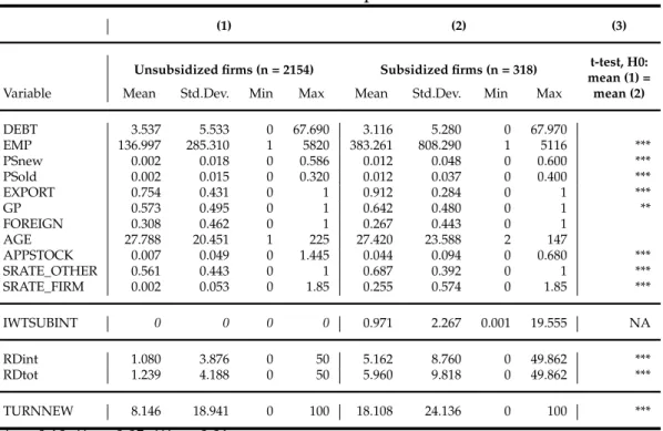
Table 1 shows some descriptive statistics for the firms included in this study, split by whether a firm received a subsidy or not.12
Column 3 presents the significance levels of two-sided t-tests on differences be-tween mean values of the variables of subsidized and unsubsidized firms. Subsidized firms are, on average, larger, more likely to be exporters and part of a group. They are
11An overview of the industry structure is given in table A.1 in appendix. 12The IWTSUBINT variable is thus 0 for all unsubsidized firms by construction.
Table 1: Descriptive Statistics
(1) (2) (3)
Unsubsidized firms (n = 2154) Subsidized firms (n = 318) t-test, H0: mean (1) =
Variable Mean Std.Dev. Min Max Mean Std.Dev. Min Max mean (2)
DEBT 3.537 5.533 0 67.690 3.116 5.280 0 67.970 EMP 136.997 285.310 1 5820 383.261 808.290 1 5116 *** PSnew 0.002 0.018 0 0.586 0.012 0.048 0 0.600 *** PSold 0.002 0.015 0 0.320 0.012 0.037 0 0.400 *** EXPORT 0.754 0.431 0 1 0.912 0.284 0 1 *** GP 0.573 0.495 0 1 0.642 0.480 0 1 ** FOREIGN 0.308 0.462 0 1 0.267 0.443 0 1 AGE 27.788 20.451 1 225 27.420 23.588 2 147 APPSTOCK 0.007 0.049 0 1.445 0.044 0.094 0 0.680 *** SRATE_OTHER 0.561 0.443 0 1 0.687 0.392 0 1 *** SRATE_FIRM 0.002 0.053 0 1.85 0.255 0.574 0 1.85 *** IWTSUBINT 0 0 0 0 0.971 2.267 0.001 19.555 NA RDint 1.080 3.876 0 50 5.162 8.760 0 49.862 *** RDtot 1.239 4.188 0 50 5.960 9.818 0 49.862 *** TURNNEW 8.146 18.941 0 100 18.108 24.136 0 100 *** * p<0.10, ** p<0.05, *** p<0.01
also more likely to have a history of innovation, reflected by a larger patent stock. In line with expectations, the summary statistics also show that subsidized firms have a larger stock of both past project applications and application success rates. On aver-age, close competitors of subsidized firms are more likely to have higher application success rates. With respect to the outcome variables, subsidized firms seem to have higher R&D intensities as well as a larger innovation output.
5
Empirical implementation and results
5.1
Innovation inputs
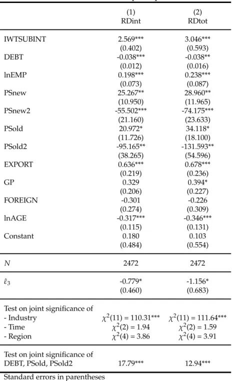
In this section we focus on input additionality effects of subsidies on the innovation input decisions of firms. Table 2 presents the impact of IWT subsidies as measured by subsidy intensity on internal R&D intensity, RDint, in column 1 and total R&D intensity, RDtot, in column 2. As the subsidy variable is possibly endogenous in this
equation it has been instrumented as outlined above. The first stage of this IV regres-sion is shown in Table A.2 in the appendix. All excluded instruments are positive and significant in the first stage and the regression does not suffer from a possible weak instrument bias, as the F-test on joint significance of the instrumental variables in the first stage amounts to a value of 12.74.
We also find support for the common opinion that the subsidy variable is an en-dogenous regressor in the R&D equation as the residuals of the first stage regression, ˆ
ε3 are significantly different from zero in the regression; at least at the 10%
signifi-cance level (see Table 2).13
The results of the R&D equation confirm a positive significant impact of the sub-sidy intensity on innovation input both when this latter is measured as internal R&D intensity and as total R&D intensity. Full crowding out can thus be rejected as subsi-dies do seem to stimulate innovation expenditures.
In order to test whether partial crowding out can be rejected, the following logic can be applied. If the subsidy rate would amount to 50% we should expect that the estimated coefficient of the subsidy variable in the R&D equation amounts at least to the value 2, because the firm would need to finance the same amount as the sub-sidy itself from private resources if the project is implemented to full extent.14 More generally, the estimated coefficient should be larger than the inverse of the subsidy rate (1/SR). The average subsidy rate in our framework is 43.395%, implying that total R&D investment should increase by at least 2.304 times the subsidies received. The results presented in table 2 suggest that this is indeed the case: the estimated coefficient is 3.046.15
13We also computed the Hansen J-test and did not reject the hypothesis that the instruments are ex-ogenous, i.e. the instruments are not only relevant in the first stage but also valid in terms of statistical requirements.
14Note that R&D spending in our case is all money invested, i.e. including the subsidy. If we would have measured R&D net of the subsidy the relevant test in the example outlined above would be whether the estimated coefficient is larger than the value 1.
15Strictly speaking we cannot reject the hypothesis of some crowding–out as a t-test reveals that the estimated coefficient of 3.046 is not significantly larger than 2.304. However, this is not the main focus of the paper and results suggest that the subsidy certainly increases private R&D investment by an economically significant factor.
Table 2: Innovation input equations (1) (2) RDint RDtot IWTSUBINT 2.569*** 3.046*** (0.402) (0.593) DEBT -0.038*** -0.038** (0.012) (0.016) lnEMP 0.198*** 0.238*** (0.073) (0.087) PSnew 25.267** 28.960** (10.950) (11.965) PSnew2 -55.502*** -74.175*** (21.160) (23.633) PSold 20.972* 34.118* (11.726) (18.100) PSold2 -95.165** -131.593** (38.265) (54.596) EXPORT 0.636*** 0.678*** (0.219) (0.236) GP 0.329 0.394* (0.206) (0.227) FOREIGN -0.301 -0.226 (0.274) (0.309) lnAGE -0.317*** -0.346*** (0.115) (0.131) Constant 0.180 0.103 (0.484) (0.554) N 2472 2472 ˆ ε3 -0.779* -1.156* (0.460) (0.683) Test on joint significance of
- Industry χ2(11) = 110.31*** χ2(11) = 111.64***
- Time χ2(2) = 1.94 χ2(2) = 1.59
- Region χ2(4) = 3.86 χ2(4) = 3.91
Test on joint significance of
DEBT, PSold, PSold2 17.79*** 12.94*** Standard errors in parentheses
The coefficients of the other control variables are, in general, in line with expecta-tions. Patent stock, both old and new, seems to have a curvilinear effect on innovation inputs. Larger firms seem to have a higher innovation input and in line with expecta-tions on their international presence, exporters invest more into innovation activities. In addition, the older the firm, the less it invests in innovation activities on average. Group members seem to have a slightly higher total R&D intensity, ceteris paribus.
Finally, the test on the joint significance of DEBT and the old patent stocks show that they may well serve as instrumental variables for the output equation as they have a strong, joint influence on R&D investment (see Table 2).
5.2
Innovation outputs
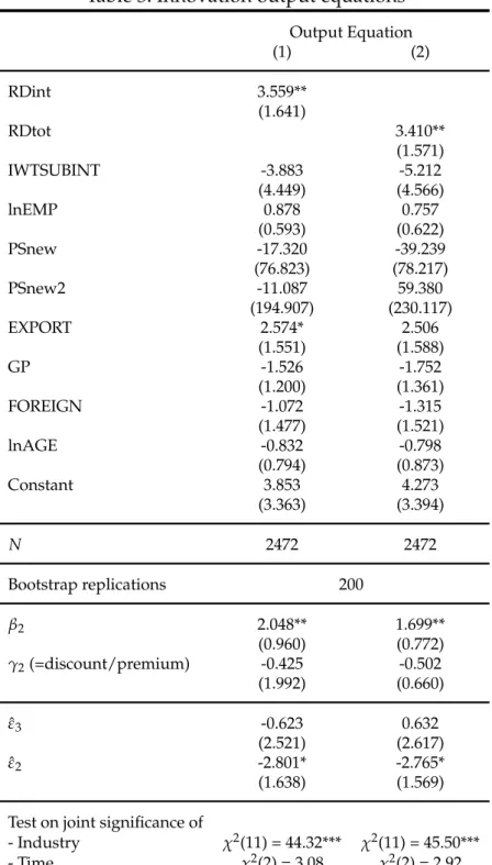
This section assesses the impact of private R&D inputs on output and analyzes to what extent a premium or discount can be found of the subsidized projects with re-spect to innovation output at the firm level. Table 3 presents the results of this esti-mation. The first column presents results when the calculation of the R&D variables is based upon internal R&D intensity (RDint) and column 2 when this is based upon total R&D intensity (RDtot).
Results show that the private part of both total R&D expenditures and internal R&D expenditures has a positive significant effect on innovation output as reflected by the coefficient of RDint and RDtot respectively. IWTSUBINT is not significant. However, as described extensively introduced before, this coefficient should not be interpreted, as it is the reduced form coefficientπ. Instead, in a first step, the structural
parameter,β2, referring to the coefficient of subsidy induced R&D, can be calculated
as introduced above: β2=β1+πα. Results in table 3 show that the subsidy induced
R&D investment has a positive significant effect on output.
Another question in this study is whether this lower coefficient of subsidized R&D reflects a lower productivity when compared to the privately invested R&D. There-fore, we could test whetherβ2is significantly different from β1, or in the logic of the
param-Table 3: Innovation output equations Output Equation (1) (2) RDint 3.559** (1.641) RDtot 3.410** (1.571) IWTSUBINT -3.883 -5.212 (4.449) (4.566) lnEMP 0.878 0.757 (0.593) (0.622) PSnew -17.320 -39.239 (76.823) (78.217) PSnew2 -11.087 59.380 (194.907) (230.117) EXPORT 2.574* 2.506 (1.551) (1.588) GP -1.526 -1.752 (1.200) (1.361) FOREIGN -1.072 -1.315 (1.477) (1.521) lnAGE -0.832 -0.798 (0.794) (0.873) Constant 3.853 4.273 (3.363) (3.394) N 2472 2472 Bootstrap replications 200 β2 2.048** 1.699** (0.960) (0.772) γ2(=discount/premium) -0.425 -0.502 (1.992) (0.660) ˆ ε3 -0.623 0.632 (2.521) (2.617) ˆ ε2 -2.801* -2.765* (1.638) (1.569) Test on joint significance of
- Industry χ2(11) = 44.32*** χ2(11) = 45.50***
- Time χ2(2) = 3.08 χ2(2) = 2.92
- Region χ2(4) = 3.29 χ2(4) = 3.32
Standard errors in parentheses * p<0.10, ** p<0.05, *** p<0.01
eter (γ2= βπ1α).
For the output equation with R&D input measured as RDint, we findγ2= (3.559−3.883∗2.569) =
0.425, suggesting thus a discount of subsidized R&D regarding the marginal pro-ductivity effect of 42.5% with respect to privately financed R&D when internal R&D speding is used as regressor. Similarly, a discount of 50.2% is suggested with respect to total R&D intensity (γ2=(3.410−5.212∗3.046)). However, as shown in table 3, these
coeffi-cients are insignificant, i.e. statistically we do not reject the hypothesis that privately financed R&D and subsidized R&D have equal marginal productivity effects.
In sum, results point to a positive significant effect on innovation output of both purely private and subsidy induced R&D. Furthermore, we do not find evidence of a lower effect of this latter component compared to privately financed R&D in terms of generated sales due to new products.
There is thus no conclusive evidence supporting either one of the arguments out-lined above, in favor of expecting a discount or suggesting a premium of subsidy induced R&D relative to private R&D in terms of innovative output.
6
Conclusion
This paper models input and output additionality in a structural model. It extends the Crépon Duguet Mairesse (CDM) framework by incorporating subsidies as a de-terminant of both the input and output equations. Thereby, this study adds to the CDM framework, the widely spread input additionality literature and the less inves-tigated output additionality strand of research. This is done by explicitly modeling the interdependency between subsidies, innovation input and output.
The empirical study is carried out using Flemish Innovation Survey data coupled with detailed subsidy data. In line with a lot of the prevalent literature, the empirical analysis finds evidence for input additionality of subsidies. In general, crowding–out can thus be rejected and public incentive schemes seem to increase R&D spending in the business sector.
In addition, this analysis reveals that, in general, an increase in private R&D inputs leads to higher innovative performance. In addition, subsidy induced R&D, encom-passing both the subsidy and the additional R&D investment due to this subsidy, also increases sales due to new products. Furthermore, there is no evidence of a lower or higher productivity of public R&D compared to private R&D. Statistically both com-ponents of firms R&D activities have similar marginal effects on sales with new prod-ucts. There is thus no evidence suggesting that policy makers either select projects with lower private value or that subsidized projects fail much more frequently than others.
Of course, our study has a number of caveats that remain for further research. A specific shortcoming of this study is that the subsidy application and granting deci-sion stages are not incorporated separately as in Takalo et al., 2013), for instance. As in numerous other studies of this kind, it would be valuable to have access to more balanced panel data that allow to control for unobserved firm-specific effects in the regressions. In addition, future research could further extend this model to heteroge-neous treatment effects in the input stage, i.e. the estimation of firm-specificαi, and
References
Aghion, P. and Howitt, P. (1998), ‘Capital accumulation and innovation as complementary factors in long-run growth’,Journal of Economic Growth3, 111–130.
Almus, M. and Czarnitzki, D. (2003), ‘The effects of public R&D subsidies on firms’ innova-tion activities: the case of Eastern Germany’,Journal of Business and Economics Statistics
21, 226–236.
Arrow, K. (1962), Economic welfare and the allocation of resources for invention,inR. Nelson, ed., ‘The rate and direction of inventive activity: economic and social factors’, Princeton University Press, pp. 609–625.
Barney, J., Wright, M. and Ketchen, D. (2001), ‘The resource-based view of the firm: ten years after 1991’,Journal of Management27, 625–641.
Blank, D. and Stigler, G. (1957), ‘The demand and supply of scientific personnel’, National Bureau of Economic Research, New York.
Busom, I. (2000), ‘An empirical evaluation of the effects of R&D subsidies’,Economics of Inno-vation and New Technology9, 111–148.
Castellani, D. and Zanfei, A. (2006),Multinational firms, innovation and productivity.
Cerulli, G. (2010), ‘Modelling and measuring the effect of public subsidies on business R&D: A critical review of the econometric literature’,The economic record.
Colombo, M. G. and Grilli, L. (2005), ‘Founders’ human capital and the growth of new technology-based firms: a competence-based view’,Research Policy34, 795–816.
Crépon, B., Duguet, E. and Mairesse, J. (1998), ‘Research, innovation and productivity: an econometric analysis at the firm level.’,Economics of Innovation and New Technology7, 115– 158.
Czarnitzki, D. and Delanote, J. (2015), ‘R&D policies for young SMEs: input and output ef-fects’,Small Business Economics45(3), 465–485.
Czarnitzki, D. and Hussinger, K. (2004), ‘The link between R&D subsidies, R&D spending and technological performance’,ZEW working paper, 4-56.
Czarnitzki, D. and Licht (2006), ‘Additionality of Public R&D Grants in a Transition Economy: the Case of Eastern Germany’,The Economics of Transition14, 101–131.
Czarnitzki, D. and Lopes Bento, C. (2012), ‘Evaluation of public R&D policies: A Cross-Country Comparison’, World Review of Science, Technology and Sustainable Development
9(2/3/4), 254–282.
David, P., Hall, B. and Toole, A. (2000), ‘Is public R&D a complement or substitute for private R&D? a review of the econometric evidence’,Research Policy29, 497–529.
Duguet, E. (2004), ‘Are R&D subsidies a substitute or a complement to privately funded R&D? evidence from France using propensity score methods for non experimental data’,Revue d’Economie Politique114, 263–292.
Geroski, P. and Toker, S. (1996), ‘The turnover of market leaders in UK manufacturing indus-try, 1979-86’,International journal of industrial organization14, 141–158.
Gonzales, X., Jaumandreu, J. and Pazo (2005), ‘Barriers to innovation and subsidy effective-ness’,RAND Journal of Economics36, 930–949.
Gonzales, X. and Pazo, C. (2008), ‘Do public subsidies stimulate private R&D spending?’,
Research Policy37, 371–389.
Goolsbee, A. (1998), ‘Does R&D Policy primarily benefit scientists and engineers?’,American Economic Review88, 298–302.
Griliches, Z. (1979), ‘Issues in assessing the contribution of research and development to pro-ductivity growth.’,Bell Journal of economics10, 92–116.
Griliches, Z. (1986), ‘Productivity, R&D and basic research at the firm level in the 1970s”,
American Economic Review76, 141–154.
Griliches, Z. (1998), Patent statistics as economic indicators: a survey,in‘R&D and productiv-ity: the econometric evidence’, University of Chicago Press, pp. 287–343.
Hussinger, K. (2008), ‘R&D and subsidies at the firm level: an application of parametric and semi-parametric two-step selection models’,Jounal of Applied Econometrics23, 729–747. Klette, T., Moen, J. and Griliches, Z. (2000), ‘Do subsidies to commercial R&D reduce market
failures? microeconometric evaluation studies’,Research Policy29, 471–495.
Lach, S. (2002), ‘Do R&D subsidies stimulate or displace private R&D? evidence from israel’,
Jounal of Industrial Economics50, 369–390.
Larosse, J. (2004), ‘Conceptual and empirical challenges of evaluating the effectiveness of in-novation policies with ’behavioral additionality’, case of IWT R&D subsidies’,IWT Flan-ders, Belgium.
Lerner, J. (1999), ‘The government as venture capitalist: the long-run impact of the SBIR pro-gram’,Journal of Business72(3), 285–318.
Mansfield, E. (1962), ‘Entry, Gibrat’s law, innovation and the growth of firms’,American Eco-nomic Review52(5), 1023 – 1051.
Mansfield, E. (1988), ‘Industrial R&D in Japan and the United States: a comparative study’,
American Economic Review78, 223–228.
Nelson, R. (1959), ‘The simple economics of basic scientific research’,Journal of political economy
49, 297–306.
Scherer, F. (1965), ‘Corporate inventive ouput, profits, and growth’,journal of political economy
73(3), 290–297.
Stiglitz, J. and Weiss, A. (1981), ‘Credit Rationing in Markets with Imperfect Information’,
American Economic Review71, 393–410.
Takalo, T., Tanayama, T. and Toivanen, O. (2013), ‘Estimating the benefits of targeted R&D subsidies’,Review of Economics and Statistics95, 255–272.
Teece, D. and Pisano, G. (1994), ‘The dynamic capabilities of firms: an introduction’,Industrial and corporate change3.
Zúñiga Vicente, J., Alonso-Borrego, C., Forcadell, F. and Galan, J. (2014), ‘Assessing the effect of public subsidies on firm R&D investment: a survey’,Journal of Economic Surveys28, 36– 67.
Appendices
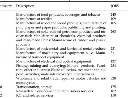
Table A.1: Industry structure
Industry Description ]OBS
1 Manufacture of food products, beverages and tobacco 245 2 Manufacture of textiles 109 3 Manufacture of wood and wood products; manufacture of
pulp, paper and paper products; publishing and printing; 105 4 Manufacture of coke, refined petroleum products and
nu-clear fuel; Manufacture of chemicals, chemical products and man-made fibres; Manufacture of rubber and plastic products
263
5 Manufacture of basic metals and fabricated metal products 231 6 Manufacture of machinery and equipment n.e.c.;
Manu-facture of transport equipment
311 7 Manufacture of electrical and optical equipment 127 8 Fishing; mining and quarrying; Mineral products;
Furni-ture; other industries; Waste collection, treatment and dis-posal activities; materials recovery; Other services
254
9 Wholesale and retail trade; repair of motor vehicles and motorcycles
320 10 Transportation, storage 175 11 Research & Development; other business services 182 12 ICT and related services 150
Table A.2: First stage : Subsidy regression (1) IWTSUBINT APPSTOCK 4.669** (2.304) SRATE_OTHER 0.105*** (0.033) SRATE_FIRM 0.864*** (0.256) DEBT 0.004 (0.003) lnEMP -0.018 (0.015) PSnew -0.566 (3.340) PSnew2 13.893* (8.426) PSold -3.698 (4.130) PSold2 23.002 (20.562) EXPORT 0.044 (0.039) GP -0.058 (0.037) FOREIGN 0.073* (0.039) lnAGE -0.028 (0.019) Constant 0.014 (0.082) N 2472
Test on joint significance of
Industry χ2(11) = 45.12***
Time χ2(2) = 1.99
Region χ2(4) = 18.14***
Standard errors in parentheses * p<0.10, ** p<0.05, *** p<0.01
Columns 1 and 4 of Table A.3 show an OLS regression of the output equation without accounting for the endogeneity of the R&D input and without including the subsidy variable. Columns 2 and 5 show OLS regressions where subsidies are included and the R&D variables are interacted with the subsidies. Columns 3 and 6 present the regressions where R&D expen-diture is calculated net of subsidies and subsidies are included as a separate regressor. All of these equations are estimating the marginal effects of R&D and subsidies not correctly as we argue in Section 3 of the paper.
Table A.3: ’Naive’ OLS innovation output equations (1) (2) (3) (4) (5) (6) RDint 0.841*** 0.985*** (0.128) (0.197) RDintnosub 0.782*** (0.143) RDtot 0.732*** 0.868*** (0.114) (0.179) RDtotnosub 0.673*** (0.128) IWTSUBINT 1.739 1.720 (1.077) (1.061) DSUB 6.252*** 6.275*** (1.590) (1.591) RDintDSUB -0.499** (0.247) RDtotDSUB -0.452** (0.222) lnEMP 1.299*** 1.105*** 1.345*** 1.293*** 1.103*** 1.344*** (0.388) (0.396) (0.389) (0.390) (0.397) (0.391) PSnew 74.257* 57.176 73.662* 71.650* 56.034 71.303* (41.736) (42.594) (41.587) (42.124) (42.881) (41.897) PSnew2 -145.870** -108.381 -157.744** -136.385* -103.402 -150.224** (73.335) (75.245) (73.093) (74.614) (76.141) (74.070) EXPORT 4.608*** 4.300*** 4.564*** 4.634*** 4.325*** 4.585*** (0.858) (0.863) (0.857) (0.857) (0.862) (0.857) GP -0.665 -0.708 -0.627 -0.685 -0.742 -0.641 (1.011) (1.011) (1.012) (1.012) (1.012) (1.012) FOREIGN -1.885* -1.567 -1.919* -1.963* -1.640 -1.995* (1.075) (1.080) (1.069) (1.076) (1.081) (1.070) lnAGE -1.761*** -1.702*** -1.730*** -1.770*** -1.700*** -1.736*** (0.563) (0.564) (0.562) (0.566) (0.566) (0.565) Constant 4.199* 4.612* 4.012 4.260* 4.612* 4.051 (2.537) (2.533) (2.547) (2.543) (2.535) (2.553) N 2472 2472 2472 2472 2472 2472
Test on joint significance of
- Industry F(11) 4.74*** 4.53*** 4.75*** 4.78*** 4.56*** 4.80*** - Time F(2) 1.47 1.79 1.61 1.49 1.77 1.63 - Region F(4) 1.44 1.48 1.32 1.44 1.47 1.31 Standard errors in parentheses
FACULTY OF ECONOMICS AND BUSINESS DEPARTMENT OF MANAGERIAL ECONOMICS, STRATEGY AND INNOVATION
Naamsestraat 69 bus 3500 3000 LEUVEN, BELGIË tel. + 32 16 32 67 00 fax + 32 16 32 67 32 [email protected] www.econ.kuleuven.be/MSI