Automatic parameter setting for
Arnoldi-Tikhonov methods
S. Gazzola, P. Novati
Department of Mathematics
University of Padova, Italy
March 16, 2012
Abstract
In the framework of iterative regularization techniques for large-scale linear ill-posed problems, this paper introduces a novel algorithm for the choice of the regularization parameter when performing the Arnoldi-Tikhonov method. Assuming that we can apply the discrepancy principle, this new strategy can work without restrictions on the choice of the regu-larization matrix. Moreover this method is also employed as a procedure to detect the noise level whenever it is just overestimated. Numerical ex-periments arising from the discretization of integral equations and image restoration are presented.
1
Introduction
In this paper we consider the solution of ill-conditioned linear systems of equa-tions
Ax=b, A∈RN×N, b∈RN, (1) in which the matrixAis assumed to have singular values that rapidly decay and cluster near zero. These kind of systems typically arise from the discretization of linear ill-posed problem, such as Fredholm integral equations of the first kind with a compact kernel; for this reason they are commonly referred to as linear discrete ill-posed problems (see [5], Chapter 1, for a background).
While working with this class of problems, one commonly assumes that the available right-hand side vectorb is affected by noise, caused by measurement or discretization errors. Therefore, throughout the paper we suppose that
b=b+e,
where b represents the unknown noise-free right-hand side, and we denote by
xthe solution of the error-free system Ax =b. We also assume that a fairly accurate estimate ofε=∥e∥is known, where ∥ · ∥denotes the Euclidean norm.
Because of the ill-conditioning ofAand the presence of noise inb, some sort of regularization is generally employed to find a meaningful approximation of
x. In this framework, a popular and well-established regularization technique is Tikhonov method, which consists in solving the minimization problem
min x∈Rn
{
∥Ax−b∥2+λ∥Lx∥2}, (2)
whereλ >0 is the regularization parameter andL∈R(N−p)×N is the regular-ization matrix (see e.g. [3] and [5], Chapter 5, for a background). We denote the solution of (2) byxλ. Common choices forLare the identity matrixIN (in this case (2) is said to be in standard form) or scaled finite differences approxima-tions of the first or the second order derivative (whenL̸=IN (2) is said to be in general form). We remark that, especially when one has a good intuition of the behavior of the solution x, a regularization matrix different from the identity can considerably improve the quality of the approximation given by the solution of (2). The ideal situation is when the features of the exact solution that one wants to preserve belong to the null space of the matrixL, since L acts as a penalizing filter (see [14] and the references therein for a deeper discussion).
The choice ofλ is also crucial, since it weights the penalizing term and so specifies the amount of regularization one wants to impose. Many techniques have been developed to determine a suitable value for the regularizing param-eter, usually based on the amount of knowledge of the error on b (again we refer to [5], Chapter 7, for an exhaustive background; we also quote the recent paper [15] for the state of the art). When a fairly accurate approximation ofε
is available (as in our case), a widely used method is the so-called discrepancy principle. It prescribes to take, as regularization parameter, the value ofλthat solves the following equation
∥b−Axλ∥=ηε, (3) where η >1 is a user-specified constant, typically very close to 1. The vector
b−Axλ is called discrepancy.
In this paper we solve (2) using an iterative scheme called Arnoldi-Tikhonov (AT) method, first proposed in [2]. This method has proved to be particu-larly efficient when dealing with large scale problems, as for instance the ones arising from image restoration. Indeed, it is based on the projection of the orig-inal problem (2) onto Krylov subspaces of smaller dimensions computed by the Arnoldi algorithm. For reasons closely related to the parameter choice strat-egy, this method has been experimented mostly when (2) is in standard form [10]. Recently, an extension which employs the generalized Krylov subspaces and that therefore can deal with general form problems, has been introduced in [14].
Here we mainly focus the attention on general form problems, but we adopt a different approach from the one derived in [14], since we work with the usual Krylov subspaces Km(A, b) = span{b, Ab, . . . , Am−1b} (or, if an approximate solutionx0is available, withKm(A, b−Ax0)). We call this method Generalized
Arnoldi-Tikhonov (GAT) to avoid confusion with the standard implementation of the AT method. The parameter choice strategy presented in this paper is extremely simple and does not require the problem (2) to be in standard form. Moreover, this new algorithm can handle rectangular matricesL, which is an evident advantage since in many applications this option is the most natural one. Our basic idea is to use a linear approximation of the discrepancy
∥b−Axm∥ ≈αm+λβm,
where xm is the mth approximation of the GAT method, and to solve with respect toλthe corresponding equation
αm+λβm=ηε.
As we shall see, the value of αm in the above equation will be just the GM-RES residual, whereasβmwill be defined using the discrepancy of the previous step. In this way, starting from an initial guessλ0, we will actually construct a
sequence of parametersλ1, λ2, ..., such that λm−1 will be used to compute xm until the discrepancy principle (3) is satisfied. We will be able to demonstrate that the the above technique is in fact a secant zero finder.
As we shall see, the procedure is extremely simple and does not require any hypothesis on the regularization matrixL. For this reason, in the paper we also consider the possibility of using the GAT method to approximate the noise level
εwhenever it is just overestimated by a quantityε > ε. In a situation like this the discrepancy principle generally yields poor results if the approximation of
ε is coarse. Anyway, our idea consists in restarting the GAT method, and to use the observed discrepancy to improve the approximation ofε step by step. The examples so far considered have demonstrated that this approach is really effective, and the additional expense due to the restarts of the GAT method does not heavily affect the total amout of work. This is due to the fact that the GAT method is extremely fast whenever an initial approximationx0is available.
The paper is organized as follows. In Section 2 we review the AT method and we describe its generalized version, the GAT method. In Section 3 we introduce the new technique for the choice ofλ. In Section 4 we display the results obtained performing common test problems, as well as some examples of image restoration. In Section 5 we suggest an extension of the previous method that allows to work even when the quantity ε is overestimated. Finally, in Section 6, we propose some concluding remarks.
2
The Arnoldi-Tikhonov method
The Arnoldi-Tikhonov (AT) method has been introduced in [2] with the basic aim of reducing the problem
min x∈RN
{
in the case ofL=IN, to a problem of much smaller dimension. The idea is to project the matrixAonto the Krylov subspaces generated byAand the vector
b, i.e., Km(A, b) = span{b, Ab, . . . , Am−1b}, with m ≪ N. The method was even introduced to avoid the matrix-vector multiplication withAT required by Lanczos type schemes (see e.g [1], [2], [8], [11]). For the construction of the Krylov subspaces the AT method uses the Arnoldi algorithm (see [16], Section 6.3, for an exhaustive background), which yields the decomposition
AVm=Vm+1Hm+1, (5)
whereVm+1 = [v1, ..., vm+1]∈RN×(m+1)has orthonormal columns which span
the Krylov subspaceKm(A, b) andv1 is defined asb/∥b∥. The matrixHm+1∈
R(m+1)×mis an upper Hessenberg matrix. Denoting byh
i,jthe entries ofHm+1,
in exact arithmetics the Arnoldi process arrests whenever hm+1,m = 0, which meansKm+1(A, b) =Km(A, b).
The AT method searches for approximations belonging toKm(A, b). In this sense, replacingx=Vmym(ym∈Rm) into (4) withL=IN, yields the following reduced minimization problem
min ym∈Rm {H m+1ym−VmT+1b 2 +λ∥ym∥ 2} , (6) sinceVT
mVm=Im. Remembering thatv1=b/∥b∥we also obtain
VmT+1b=∥b∥e1, wheree1= (1,0, ...,0)
T ∈Rm+1.
Looking at (6), we can say that the AT method can be regarded to as a reg-ularized version of the GMRES. We remark that a variant of this method, the so called Range Restricted Arnoldi-Tikhonov (RRAT) method, has been proposed in [10]. The RRAT method consists in starting the Arnoldi process with v1 = Ab/∥Ab∥, i.e. to work with the Krylov subspaces Km(A, Ab) = span{Ab, A2b, ..., Amb}, which leads again to (6), but with a different Hm+1
and Vm+1. The basic aim of this variant, which in general can be applied to
many Krylov solver, is to reduce the noise contained in b, at the beginning, considering the productAb. For both methods (AT and RRAT) the solution of (4) is then approximated byxm=Vmym.
The method considered in this paper is an extension of the AT method in order to work with a general regularization operator L ̸= IN and with an arbitrary starting vectorx0. We consider the minimization problem
min x∈RN { ∥Ax−b∥2+λ∥L(x−x0)∥ 2} , (7)
which is a slight modification of (4) that allows to incorporate an initial approx-imationx0 of the exact solution (eventually, ifx0 is not available, we consider
x0= 0 and we definitely solve (4)). We search for approximations of the type
where Vm ∈ RN×m is defined as in (5), except that now its columns form an orthonormal basis of the Krylov subspaceKm(A, r0), where r0 =b−Ax0.
Substituting (8) into (7) we obtain the reduced minimization problem min ym∈Rm { ∥AVmym−r0∥ 2 +λ∥LVmym∥ 2} = min ym∈Rm { ∥Hm+1ym− ∥r0∥e1∥ 2 +λ∥LVmym∥ 2} ,
which can be rewritten as the following least square problem min ym∈Rm ( √Hm+1 λLVm ) ym− ( ∥r0∥e1 0 ) 2. (9)
In the sequel we will refer to the above reduced minimization problem as Gen-eralized Arnoldi-Tikhonov (GAT) method.
We note that the problem (9) has a coefficient matrix of dimension [(m+1)+ (N−p)]×m, since, in general,L∈R(N−p)×N. At a first glance, this formulation could seem computationally disadvantageous, if compared to (6), where the ma-trixLVmis replaced by the identity matrix of ordermand the coefficient matrix of the corresponding least square problem has dimension (2m+1)×m. However, we remark that the GAT method can deal with arbitrary regularization matrices so that this drawback is usually balanced by the positive effect that a suitableL
can have on noisy problems. Furthermore, it is very important to observe that the GAT method and, in general, each Krylov solver based on the construction of the Krylov subspacesKm(A, b), is generally very fast for discrete ill-posed problems, and hence the number of columns of the matrix in (9) is very small; therefore this computational disadvantage is actually negligible, as revealed by many numerical experiments. Of course, with the word “fast” we just mean that the approximations rapidly achieve the best attainable accuracy since for this kind of problems an iterative solver typically exhibits semiconvergence or, at best, stagnates.
3
The parameter selection strategy
As already said in the Introduction, we assume to knowε=∥b−b∥. Under this hypothesis, it turns out that a successful strategy to define a suitable regular-ization parameter, as well as a stopping criterium, is the discrepancy principle (3) adapted to the iterative setting of the AT (or GAT) method. At each it-eration we can define the function ϕm(λ) =∥b−Axm,λ∥ and we say that the discrepancy principle is satisfied as soon as
ϕm(λ)≤ηε,
whereη'1. We remark that if we rather know the norm of the relative amount of noiseεe=∥e∥/∥b∥, then the discrepancy principle reads
The quantityεeis commonly referred to as noise level.
For the GAT method in which the approximations are of the form xm,λ = x0+Vmym,λ ∈x0+Km(A, r0), whereym,λ solves (9), the discrepancy can be rewritten as
∥b−Axm,λ∥=∥r0−AVmym,λ∥=∥c−Hm+1ym,λ∥, (10) wherec=VT
m+1r0=∥r0∥e1∈Rm+1. Sinceym,λ solves the normal equation (HmT+1Hm+1+λVmTL
TLV
m)ym,λ=HmT+1c,
associated to the least square problem (9), by (10) we obtain
ϕm(λ) =Hm+1(HmT+1Hm+1+λVmTL TLV
m)−1HmT+1c−c. (11)
Dealing with expressions of type (11) for the discrepancy, a standard ap-proach consists in solving, with respect toλ, the nonlinear equation
ϕm(λ) =ηε. (12)
In [12] the authors present, for the case L = IN, a cubically convergent zero finder which involves quantities that can be computed quite cheaply. The strat-egy adopted in [10] is to first determine a suitable value ofm(that assures that the equation (12) has a unique solution) and then apply the above mentioned cubic zero finder. However the value ofminitially determined may be too small to guarantee a good approximation and usually one or two extra iterations are performed to improve the quality of the solution.
Using the method that we are going to describe, suitable values for λand
mare determined simultaneously. Our basic hypothesis is that the discrepancy can be well approximated by
ϕm(λ)≈αm+λβm, (13) i.e., a linear approximation with respect to λ, in which αm, βm ∈ R can be easily computed or approximated. For what concernsαm, the Taylor expansion of (11) suggests to chose
αm=ϕm(0) =Hm+1(HmT+1Hm+1)−1HmT+1c−c,
which is just the norm of the residual of the GMRES, which can be evaluated working in reduced dimension, independently of the choice ofL. In accordance with our notations, we denote byym,0 the projected GMRES solution, i.e., the
solution of
min
y∈Rm∥Hm+1y−c∥. (14)
For what concerns βm, suppose that, at the step m, we have used the pa-rameterλm−1(computed at the previous step or, ifm= 1, given by the user) to
computeym,λm−1, by solving (9) with λ=λm−1. Then we can easily compute
the corresponding discrepancy by (10)
ϕm(λm−1) =c−Hm+1ym,λm−1, (15)
and consequently, using the approximation (13), we obtain
βm≈
ϕm(λm−1)−αm λm−1
. (16)
To selectλmfor the next step of the Arnoldi algorithm we impose
ϕm+1(λm) =ηε, (17) and force the approximation
ϕm+1(λm)≈αm+λmβm. (18) Hence by, (16) and (17), we define
λm=
ηε−αm ϕm(λm−1)−αm
λm−1. (19)
The method (19) has a simple geometric interpretation which allows to see it as a zero finder. Indeed, we know thatϕm(λ) is a monotonically increasing function such thatϕm(0) =αm(cf. also [10]). Hence, the linear function
f(λ) =αm+λ ( ϕm(λm−1)−αm λm−1 ) ,
interpolates ϕm(λ) at 0 andλm−1, and the new parameter λm is obtained by solving f(λ) = ηε. Hence (19) is just a secant method in which the leftmost point is (0, αm). In the very first steps of (19) instability can occur: this is due to the fact that we may haveαm> ηε. In this situation the result of (19) may be negative and therefore we use
λm= ηε−αm ϕm(λm−1)−αm λm−1. (20)
Anyway, we know that, independently of the definition of λm−1, after some
stepsαm< ηε(compare also the arguments given in [10]) so that (20) actually represents one step of a zero finder. In Figure 1 we display what typically happens at them-th iteration of the GAT method when the conditionαm< ηε is satisfied.
Numerically, formula (20) is very stable, in the sense that after the dis-crepancy principle is satisfied, λm ≈ const. This is due to the fact that both ϕm(λm−1) and αm = ϕm(0) stagnates. Indeed, since the approxima-tions are computed minimizing the residual within a Krylov subspace, when-everKm+1(A, b) ≈ Km(A, b), the values of ϕm(λm−1) and αm =ϕm(0) tends to remain almost constant because, in any case b−AVmym,λ ∈ Km+1(A, b),
even if the solutions of (9), ym,λm−1, and the one of GMRES, ym,0, are badly
φm(λ)
ηε
αm
λm−1 λm
Figure 1: Zero finder interpretation of formula (19).
Remark 1 It is interesting to observe that formula (19) is somehow related to the standard techniques used for approximating the local error of a discrete method for ordinary differential equations, whenever a stepsize selection strategy
is adopted. Indeed, for a method of orderp, the local error at the instanttmin
the interval of integration is of the type
LEm=cmhpm+1,
where cm is an unknown constant depending on the method and the problem,
andhm is the stepsize previously selected. Since an approximation of LEm is
generally known, i.e.,LEm≈LEm∗, we have
cm≈ LEm∗ hpm+1 .
In this way, to define the new stepsizehm+1, one imposes
LEm+1=cm+1h
p+1
m+1≤ϵ,
whereϵis the prescribed tolerance; forcing cm+1=cm yields the method
hm+1= ( ϵ LEm∗ ) 1 p+1 hm.
In (19) the role ofLEm andcm is played byϕm(λm−1)andβmrespectively.
While not considered in this paper, we remark that this parameter choice technique can also be used together with the Range-Restricted approach [10] and even in the case of Krylov methods based on the Lanczos unsymmetric
process [2]. As already mentioned in the previous sections we again emphasize the fact that the method just described can work without hypothesis on the reg-ularization matrix L, and that essentially involves quantities that are strictly connected to the projected problem. At each iteration we simply have to mon-itor the value ofϕm(λ) for λ= 0 and λ= λm−1, so that the only additional
cost is due to the computation (in reduced dimension) of the GMRES residual, attainable inO(m2) operations (if the QR update is not employed, otherwise in
justO(m) operations).
If compared to the other parameter choice strategies so far used in connection with the AT method, we realize that the present one is intrinsically simpler and cheaper. In fact, if at each iteration we want to apply the L-curve criterium to the standard form reduced problem (6), as proposed in [2] where this algorithm is referred to asLm-curve method, we have to compute the SVD of Hm+1 in
order to solve the system (9) for many values ofλ. Then we need to employ a reliable algorithm to choose the point of maximum curvature, that sometimes may even provide an unsatisfactory value forλ. On the other side, using the method proposed in [10], once determined a suitable m, we have to apply a convergent zero-finder to solve the nonlinear equation (12). The latter requires, at each step, the value of the first and the second derivative ofϕmcomputed for theλdetermined at the previous step and to do this we have to solve two linear systems of dimensionm. Actually, since in both cases all the extra computations involve the reduced matrices, we also stress that the computational overload can still be considered negligible. However, the generalization of these strategies to the case of the GAT method is not straightforward: we believe that the most accessible approach is to first transform the problem (4) into standard form (by employing, e.g., theA-weighted pseudoinverse ofL) and then apply the AT method to the transformed problem. Anyway this approach is not as general as the GAT method since, in order to obtain a square matrix associated to the transformed problem,Lmust be square itself (as explained in [13]). Moreover, this initial transformation affects the overall computational cost because the operations are of course in full-dimension.
Below we present the algorithm used to implement the method.
Algorithm 2 Generalized Arnoldi-Tikhonov
Input: A,b,L,x0,λ0,ε,η
Form= 1,2, ...until∥b−Axm,λ∥ ≤ηε
1. UpdateVm,Hm+1 with the Arnoldi algorithm (5);
2. Solve (9) with λ=λm−1 and evaluateϕm(λm−1) by (15);
3. Compute the GMRES solution and evaluate αm=ϕm(0);
4
Computed examples
To support the new method (20), that from now on we callsecant update, we show some numerical experiments. In particular, when possible, we compare the performance of our formula with respect to the ones proposed in [2] and [10]. In all the examples we suppose to know the exact solutionxand the exact right-hand side vector is constructed takingb=Ax. The elements of the noise vector
eare normally distributed with zero mean and the standard deviation is chosen such that ∥e∥/∥b∥ is equal to a prescribed level εe. In this section we always take the initial guess x0 = 0 and set η = 1.001. All the computations have
been executed using Matlab 7.10 with 16 significant digits on a single processor computer Intel Core i3-350M.
Example 1. We consider a problem coming from a first-kind Fredholm integral equation used to model a one-dimensional image restoration process
∫ π/2 −π/2 K(s, t)f(t)dt = g(s), −π/2≤s≤π/2, (21) where K(s, t) = (cos(s) + cos(t))2 ( sin(u) u )2 , u=π(sin(s) + sin(t)), f(t) = 2 exp(−6(t−0.8)2) + exp(−2(t+ 0.5)2).
We use the Matlab codeshaw.m from [4] in order to discretize (21) using 200 collocation points defined byti= (i−0.5)π/200,i= 1, . . . ,200 and to produce a symmetric matrixA∈R200×200and the solutionx. The condition number of
Ais around 1020. We will consider a noise levelεe= 10−3.
In order to present a straightforward comparison with the methods com-monly used in connection with the AT method, in this first example we will take L = I200. In this context, when we employ the Lm-curve criterium, we stop at iterationme if the norm of the discrepancy associated to the parameter computed using theLme-curve is below the known thresholdηε.
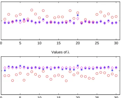
In Figure 2 we display the results obtained performing 30 tests (for each test we defined a new perturbed right-hand side to lessen the dependence of the results on the random components of e). Both the Lm-curve and the secant update method determine a regularized solution which always belongs to the Krylov spaceK8(A, b). However the new method is in every situation the more
stable one, since the relative error norms and the values ofλdetermined during the last iteration are always comparable. The same does not hold for theLm -curve method, that on average produces approximated solutions of slightly worse quality. We also show the norms of the relative error and the values of the regularization parameter determined solving the nonlinear equationϕ8(λ) =ηε
by Newton’s method.
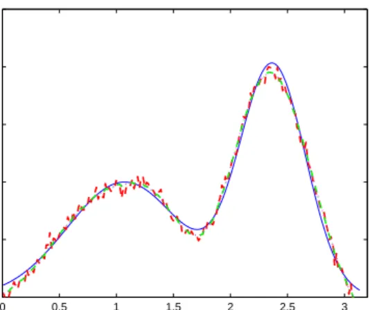
In Figure 3 we plot the solution, corresponding to the test #8 reported in Figure 2, computed using theLm-curve criterium and our secant approach. We
0 5 10 15 20 25 30 10−1.5 10−1.3 10−1.1 Relative Errors 0 5 10 15 20 25 30 10−10 10−5 Values of λ
Figure 2: The norms of the relative error (above) and the values of λ at the corresponding to the last iteration (below) for each one of the 30 tests performed. The asterisk denotes the secant update method, the circle denotes theLm-curve method and the diamond denotes the values obtained solvingϕ8(λ) =ηε.
can see that, employing Tikhonov regularization method in standard form, the quality of the solution obtained using both methods are comparable, but the one computed by theLm-curve method shows instability around the solution. This is due to the fact that this criterium allows a slight undersmoothing since it typically selects values ofλsmaller than the secant update method (cf. Figure 2).
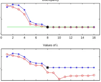
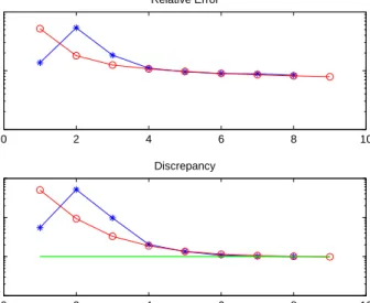
In Figure 4 we compare the behavior of theLm-curve method and the one of our secant update at each iteration. The results correspond to the test #22 re-ported in Figure 2. Since, in this example, the discrepancy principle is satisfied after only 8 iterations, we decide to compute some extra iterations to evaluate the behavior of both methods after the stopping criterium is fulfilled. In partic-ular, we can note that the secant approach exhibits a very stable progress since, once the threshold is reached, the norm of the discrepancy stagnates and the values of the regularization parameterλremain almost constant.
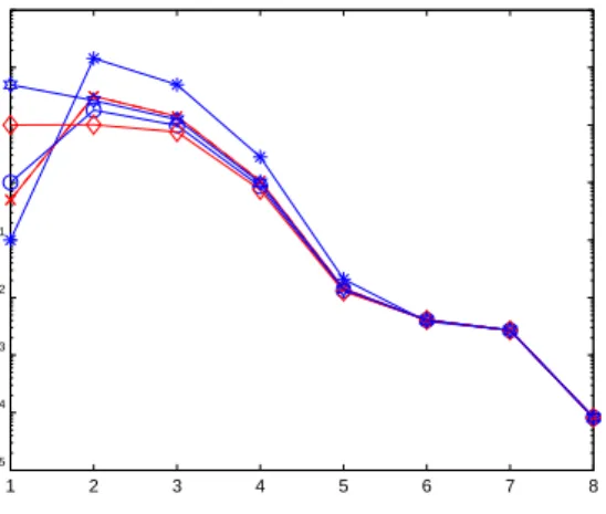
In Figure 5 we display the values of the regularization parameter, at each iteration, obtained varying the initial value λ0 given in input. We choose
de-0 0.5 1 1.5 2 2.5 3 0 0.5 1 1.5 2 2.5
Figure 3: Computed solutions of Example 1. Exact solution (solid line), regu-larized with the secant update (dash-dot line), reguregu-larized with the Lm-curve method (dashed line).
termine a suitable value of λ independently of the choice of the initial guess. As already said, at the beginning we just forceλm to be positive by (20), and then everything is handled by the conditionαm< ηε. Whenever this condition is satisfied, (20) is just a zero finder, so that the curves ofλoverlap after some steps.
Example 2. We now consider some examples coming from 2D image restora-tion problems. In particular we will focus on the deblurring and denoising of grayscale images, which consists in recovering then×noriginal imageX from an available blurred and noisy one B (see [7] for a background). To describe these problems we will obviously adopt a linear model and therefore we write the unknown exact image as x = vect(X) ∈ RN, N = n2. We will always
consider a Gaussian Point-Spread Function (PSF) defined by
hσ(x, y) = 1 2πσ2exp ( −x2+y2 2σ2 ) ,
and zero boundary conditions. This lead to a symmetric Toeplitz matrix given by
A= (2πσ2)−1T⊗T ∈RN×N,
where T ∈ Rn×n is a symmetric banded Toeplitz matrix whose first row is a vectorvdefined by
vj= {
e−(j2−σ1)22 for j = 1, . . . , q,
0 2 4 6 8 10 12 14 16 10−4 10−2 100 Discrepancy 0 2 4 6 8 10 12 14 16 10−5 100 Values of λ
Figure 4: Comparison between the values of the norm of the discrepancy and the values of the regularization parameter computed, at each iteration, by the
Lm-curve method (circles) and by the secant update (asterisks). The horizontal line in the upper graphic represents the thresholdηε. The values corresponding to the 8th iteration, the one at which both methods would stop, are marked with a ticker asterisk.
The parameter q is the half-bandwidth of the matrix T, and the parameter
σ controls the shape of the PSF (the larger σ, the wider the function). The boundary conditions are set to zero. We use Hansen’s functionblur.m from [6] to build the blurring matrixA. We consider a noise level eε= 10−2 and, as
stated at the beginning of this section, we construct the corrupted image, in vector form, asb=Ax+e.
In this context, we will exclusively consider Tikhonov regularization in gen-eral form. In the following we list the main regularization matrices that we have employed. We display the matrices in rectangular form and we use the notation ˆ
L when we consider their square versions obtained by appending or prepend-ing a suitable number of rows in such a way that the bidiagonal or tridiagonal
1 2 3 4 5 6 7 8 10−5 10−4 10−3 10−2 10−1 100 101 102 103
Figure 5: The value of the regularization parameter computed at each iteration by the secant update method, varying the initial guessλ0.
pattern of the original matrix is preserved.
L1 : = 1 −1 . .. . .. 1 −1 ∈R(N−1)×N, (22) L1L : = ( In⊗L1 L1⊗In ) ∈R2n(n−1)×N, (23) L1M : =In⊗Lˆ1+ ˆL1⊗In ∈RN×N, (24) L2 : = 1 −2 1 . .. . .. . .. 1 −2 1 ∈R(N−2)×N, (25) L2L : =In⊗Lˆ2+ ˆL2⊗In ∈RN×N. (26) The operators (22) and (25) represent scaled finite difference approximations of the first and the second derivative, respectively; sometimes The operator (23) is taken from [9], the matrix (26) represents a discretization of the two dimensional Laplace operator. We also introduce the matrix (24) that is the sum of the discretized first derivatives in the vertical and horizontal direction.
Our first task is to compare the performance of theLm-curve criterium and of the new method. We consider the popular test image peppers.png, in its original size 256×256 pixels. The corresponding linear system has dimension 65536. We corrupt the original image using a Gaussian blur whose parameter is
σ= 2.5; we setq= 6,εe= 10−2and we takeL
2as regularization matrix. In order
functioncgsvd.m, belonging to the same package, with the purpose of working with the matrixL2Vk which has more rows than columns. In Figure 6 we can examine the quality of the reconstruction obtained using both the Lm-curve criterium (box (c)) and the secant approach (box (d)). In Figure 7 we report the history of the norm of the relative error and of the discrepancy for both methods. We can see that the restored images are almost identical, even if the norm of the relative error is equal to 7.88·10−2if we use theL
m-curve method and 8.34·10−2 if we use our secant approach; the number of iterations is 9 in the first case, 8 in the second case. However, considering the running time, the difference between the two approaches is more pronounced: using theLm-curve criterium we need 3.05 seconds to compute the solution, while the new method restores the available image in 0.49 seconds. This gap is mainly due to the fact that, using the Lm-curve method, at each step we have to evaluate the Generalized Singular Value Decomposition (GSVD) of the matrix pair (Hk+1, L2Vk) and the dimension of second matrix is the same of the unreduced problem.
(a) (b)
(c) (d)
Figure 6: Original image peppers.png (a), blurred and noisy image(b), re-stored image with the Lm-curve criterium (c) and restored image with the secant update method(d).
We now focus exclusively on our method. We want to test the behavior of the GAT method varying the regularization matrix. As a matter of fact the corrupted image is always restored in less than a second and the results obtained
0 2 4 6 8 10 10−2 10−1 100 Relative Error 0 2 4 6 8 10 10−3 10−2 10−1 100 Discrepancy
Figure 7: Restoration of peppers.png. Comparison between the norm of the relative error (above) and the norm of the discrepancy (below) obtained us-ing the Lm-curve criterium (circles) and the secant update (asterisks). The horizontal continuous line marks the thresholdηε.
using different regularization matrices taken from the list (22)-(26) are very similar. In particular, since the test image is smooth and lacks of highly definite edges, the best result is obtained applying the second derivative operatorL2. To
improve the quality of the restoration, once the stopping criterium is fulfilled at a certain step withλas regularization parameter, we try to carry on some extra iterations with λ fixed. We will denote this approach with the abbreviation
Lt,ex, wheretis one of the subscripts presented in (22)-(26) andexdenotes the number of extra iterations performed.
In Table 1 we record the results obtained considering an underlying Gaussian blur function with σ = 1.5. The results displayed in Table 2 are relative to
σ= 2.5. The parameterqis set equal to 6 and the noise leveleεis equal to 10−2
in both cases.
Finally we consider the performance of the new method applied to the restoration of corrupted medical images. We take the test imagemri.tiffrom Matlab, of size 128×128 pixels, which represents a magnetic resonance image of a section of the human brain. Contrary to the previous test image, the present one is characterized by well marked edges. We again consider a Gaussian blur with parameter σ = 1.5. The half-bandwidth of T is q = 6 and the noise level is equal to 10−2. In Table 3 we report the results obtained changing the
Reg. Matr. Relative Error Iterations Running time (sec) IN 7.3930·10−2 4 0.21 L1 5.5585·10−2 6 0.34 L1L 5.5594·10−2 6 0.39 L1M 5.5665·10−2 6 0.31 L1M,4 5.0402·10−2 10 0.62 L2 5.2268·10−2 7 0.39 L2L 5.2423·10−2 7 0.40 L2L,4 5.0298·10−2 11 0.79
Table 1: Results of the restoration ofpeppers.pngaffected by a Gaussian blur with σ = 1.5 and a noise level equal to 10−2. In the first column we list the
regularization matrices considered.
Reg. Matr. Relative Error Iterations Running time (sec)
IN 1.1268·10−1 6 0.23 L1 8.4488·10−2 8 0.48 L1L 8.4487·10−2 8 0.53 L1M 8.4446·10−2 8 0.47 L1M,3 7.6920·10−2 11 0.73 L2 8.3142·10−2 8 0.47 L2L 8.3742·10−2 8 0.47 L2L,3 7.6927·10−2 11 0.80
Table 2: Results of the restoration ofpeppers.pngaffected by a Gaussian blur with σ = 2.5 and a noise level equal to 10−2. In the first column we list the regularization matrices considered.
employing the regularization matrixL1M and running the GAT algorithm for 5 extra iterations.
5
Noise level detection
The Generalized Arnoldi-Tikhonov method used in connection with the param-eter selection strategy presented in Section 3 can be successfully employed also to estimate the noise levelε/b if it is not a-priori known. In a situation like this, the discrepancy principle may yield poor results and other techniques such as the L-curve criterium or the GCV method are generally used (here we again quote [15] for a recent overview about the existing parameter choice strategies). If we assume that that εis overestimated by a quantity ε, we may expect that applying the GAT method we can fully satisfy the discrepancy principle
Reg. Matr. Relative Error Iterations Running time (sec) IN 1.8615·10−1 6 0.07 L1 1.8459·10−1 6 0.10 L1L 1.8471·10−1 6 0.10 L1M 1.8434·10−1 6 0.08 L1M,5 1.7078·10−1 11 0.17 L2 1.7704·10−1 8 0.11 L2L 1.7700·10−1 8 0.11 L2L,5 1.6854·10−1 13 0.27
Table 3: Results of the restoration ofmri.tifaffected by a Gaussian blur with
σ= 1.5 and a noise level equal to 10−2.
even takingη= 1, that is,
ϕm(λm−1)< ε, (27)
for a givenm. Applying the secant update method (20) for the definition of the parameterλ, the discrepancy would then stabilize around ε, if the method is not arrested (cf. Figure 4). Our idea is to restart it immediately after (27) is fulfilled, working with the Krylov subspaces generated byAandb−Axm,λm−1,
wherexm,λm−1 is the last approximation obtained. At the same time we define ε:= ϕm(λm−1) as the new approximation of the noise. We proceed until the
discrepancy is almost constant and we introduce a threshold parameter δ to check this situation step-by-step. This idea has been implemented following the algorithm given below.
Algorithm 3 Restarted Generalized Arnoldi-Tikhonov
Input: A,b,L,λ(0),η,δ, andε 0=ε > ε. Define x(0)= 0. Fork= 1,2, ...until ∥εk−εk−1∥ ∥εk−1∥ ≤ δ. (28)
1. Run Algorithm 2 with x0 =x(k−1), ε =εk−1, λ0 = λ(k−1). Let x(k) be
the last approximation achieved,ϕ(k)the corresponding discrepancy norm,
andλ(k) the last parameter value;
2. Defineεk :=ϕ(k);
3. Defineλ(k)=ϕϕ(k(−k)1)λ
(k).
We remark that Step 3 of the above algorithm is rather heuristic. Indeed, Algorithm 2 does not provide a further update forλwhenever the discrepancy principle is satisfied, since it is assumed to remain almost constant (cf. Figure 4 and 7). Anyway, in this situation, we may expect that improving the quality of the noise estimate, we haveϕ(k)≤ϕ(k−1), so that the corresponding estimated
(A) (B) (C)
Figure 8: Restoration of mri.tif using L1M,5. Original image (A), blurred
and noisy image(B), restored image(C).
in practice. The definition in Step 3 ensures thatλ(k)≈constwheneverϕ(k)≈
ϕ(k−1) (cf. (20)).
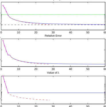
We test the procedure just described, with and without Step 3 of Algorithm 3, considering again the test imagemri.tifand, as before, we build the blurring matrix A with parameters σ = 1.5 and q = 6. Then we corrupt the blurred image in order to obtain ε/∥b∥ = 10−3. At this point we assume to know only an overestimateε, such thatε/∥b∥= 10−2. We employ the regularization matrixL1M defined by (24). In Figure 9 we display the results. We can clearly observe that, after 4 iterations, that is, after the first call of the GAT method, the norm of the discrepancy lays below the overestimated threshold ε At this point we allow the GAT method to restart immediately and to go on until the approximation is satisfactory. The implementation with δ = 0.01, including the last line of Algorithm 3, fulfils the condition (28) after 24 restarts with an estimateε24/∥b∥ = 1.03·10−3, while the version without it needs 56 restarts
to deliver the estimateε56/∥b∥= 1.05·10−3; in the first case the total running
time is 0.48 seconds, in the second case the total running time is 1.45 seconds. In this example, after the first call, the discrepancy principle is always satisfied after the first iteration. If we do not include the update described at Step 3, the
value ofλconsidered at each restart is equal to the one computed at the end of the first call. 0 10 20 30 40 50 60 10−2 10−3 Discrepancy 0 10 20 30 40 50 60 10−0.8 10−0.7 10−0.6 Relative Error 0 10 20 30 40 50 60 10−2 100 10−3 Value of λ
Figure 9: Results of Algorithm 3 applied to the restoration of mri.tif with overestimated noise level. In the first box we also plot two horizontal lines, which represent the overestimated and the true noise level. In each box, the initial 4 iterations, corresponding to the first call of Algorithm 2, are highlighted using a small circle. The continuous line represents the slower version of Algorithm 3 (without Step 3), the dashed line represents its quicker version (with Step 3).
In Figure 10 and 11 we compare the quality of the reconstruction after the first call (when the overestimated discrepancy principle is satisfied) and at the end of the scheme using Step 3 of Algorithm 3.
The numerical experiments performed on various kind of discrete ill-posed problems has proved that this approach is really robust and fairly accurate. We have not found examples in which the procedure failed. The method is restarted many times until the discrepancy is almost constant and this constant is much close to the real noise level.
We remark that generally each restart of the method allows to satisfy (27) after the first step of the Arnoldi algorithm, and hence without an heavy extra work. Anyway, since the discrepancy typically stagnates, one may even try to
(i) (ii)
(iii) (iv)
Figure 10: Restoration ofmri.tif. Original image(i), blurred and noisy image
(ii), restoration after the first 4 steps(iii), restoration with Algorithm 3 after 24 restarts(iv).
employ a rational extrapolation to avoid too many restarts, and then apply Algorithm 2 using the extrapolated value.
6
Conclusions
In this paper we have proposed an approximated version of the classical dis-crepancy principle that can be easily coupled with the iterative scheme of the Arnoldi-Tikhonov method, since it simultaneously determines the best value of the regularization parameterλ and the dimension m of the reduced problem. This technique is considerably fast and simpler than others commonly used, since it only exploits quantities that are naturally related to the problem we want to solve. The numerical experiments that we have performed so far show that the results computed by our new algorithm are comparable, if not better, to the results computed using the most established methods. Moreover, the ro-bustness and the simplicity of the approach described allows to employ it even as noise-level detector, as demonstrated experimentally in Section 5.
(i) (ii) (iii) (iv)
Figure 11: Restoration ofmri.tif. Blow-up of the corresponding images shown in Figure 10.
be successfully employed to regularize huge ill-posed linear problems coming from many applications, especially the ones concerning the deblurring and de-noising of corrupted images.
References
[1] ˚A. Bj¨orck, A bidiagonalization algorithm for solving large and sparse
ill-posed systems of linear equations, BIT 28 (1988) 659 670.
[2] D. Calvetti, S. Morigi, L. Reichel, F. Sgallari,Tikhonov regularization and
the L-curve for large discrete ill-posed problems, J. Comput. Apll. Math.
123 (2000) 423-446.
[3] M. Hanke, P.C. Hansen, Regularization methods for large-scale problems, Surv. Math. Ind. 3 (1993) 253-315.
[4] P.C. Hansen, Regularization Tools: A Matlab package for analysis and
[5] P.C. Hansen, Rank-Deficient and Discrete Ill-Posed Problems. Numerical
Aspects of Linear Inversion. SIAM, Philadelphia, 1998.
[6] P.C. Hansen,Regularization Tools version 3.0 for Matlab 5.2, Numer. Al-gorithms, 20 (1999), pp. 195-196.
[7] P.C. Hansen, J.G. Nagy, D.P. O’Leary,Deblurring Images. Matrices,
Spec-tra and Filtering. SIAM, Philadelphia, 2006.
[8] M.E. Kilmer, D.P. O’Leary,Choosing regularization parameters in iterative
methods for ill-posed problems, SIAM J. Matrix Anal. Appl. 22 (2001) 1204
1221.
[9] M.E. Kilmer, P.H. Hansen, M.I. Espa˜nol, A projection-based approach to
general-form Tikhonov regularization, SIAM J. Sci. Comput. 29 (2007), no.
1, 315–330
[10] B. Lewis, L. Reichel,Arnoldi-Tikhonov regularization methods, J. Comput. Appl. Math 226 (2009) 92-102.
[11] D.P. O’Leary, J.A. Simmons, A bidiagonalization-regularization procedure
for large-scale discretizations of ill-posed problems, SIAM J. Sci. Statist.
Comput. 2 (1981) 474 489.
[12] L. Reichel, A. Shyshkov, A new zero-finder for Tikhonov regularization, BIT 48(2008) 627-643.
[13] L. Reichel, Q. Ye,Simple square smoothing regularization operators, Elec-tron. Trans. Numer. Anal. 33 (2009) 63-83.
[14] L. Reichel, F. Sgallari, Q.Ye, Tikhonov regularization based on
generalized Krylov subspace methods, Appl. Numer. Math. (2010),
doi:10.1016/j.apnum.2010.10.002 (article in press).
[15] L. Reichel and G. RodriguezOld and new parameter choice rules for
dis-crete ill-posed problems. Submitted, 2012.
[16] Y. SaadIterative methods for Sparse Linear Systems, 2nd edition, SIAM, Philadelphia, 2003.