Robust Routing vs Dynamic Load-Balancing A Comprehensive Study and New Directions

Robust Routing vs Dynamic Load-Balancing

A Comprehensive Study and New Directions

Pedro Casas

, Federico Larroca

, Jean-Louis Rougier

and Sandrine Vaton

‡_{Universidad de la Rep´ublica, Montevideo, Uruguay}

Abstract—Traffic Engineering (TE) has become a challenging task for network management and resources optimization due to traffic uncertainty and to the difficulty to predict traffic varia-tions. To address this uncertainty in a robust and efficient way, two almost antagonist approaches have emerged during the last years: Robust Routing and Dynamic Load-Balancing. The former copes with traffic uncertainty in an off-line preemptive fashion, computing a stable routing configuration that is optimized for a large set of possible traffic demands. The latter balances traffic among multiple paths in an on-line reactive fashion, adapting to traffic variations in order to optimize a certain cost-function. Much has been said and discussed about the advantages and drawbacks of each approach, but very few works have tried to compare the performance of both mechanisms, particularly in the same network and traffic scenarios. This paper brings insight into several Robust Routing and Dynamic Load-Balancing algorithms, evaluating their virtues and shortcomings and presenting new mechanisms to improve previous proposals. Among others, such a study intends to help network operators in choosing an adequate mechanism to cope with traffic uncertainty.

Index Terms—Traffic Uncertainty, Stable and Reactive Robust Routing, Dynamic Load Balancing.

I. INTRODUCTION

As network services and Internet applications evolve, net-work traffic is becoming increasingly complex and dynamic. The convergence of data, telephony and television services on an all-IP network directly translates into a much higher variability and complexity of the traffic injected into the network. Recent Internet traffic studies from major network technology vendors like Cisco Systems forecast the advent of the Exabyte era [1], a massive increase in network traffic driven by high-definition video. Furthermore, current evolution and deployment-rate of broadband access technologies (e.g. Fiber To The Home) is such that the assumption of infinitely provisioned core links will soon become obsolete. Thus, simply upgrading link capacities may no longer be an econom-ically viable solution. To make matters worse, the presence of unexpected events such as network equipment failures, large-volume network attacks, flash crowd occurrences and even external routing modifications induces large uncertainty in traffic patterns. In the light of this traffic scenario, network operators are searching for reliable routing mechanisms. The term reliabilityrefers to the ability of the network to perform This work was partially funded by CELTIC project TRANS and FP7 project Euro-NF

and maintain its functions in usual circumstances, as well as under unexpected events. Two almost antagonist approaches have emerged in the recent years to cope with both the traffic increasing dynamism and the need for cost-effective solutions: Robust Routing (RR) and Dynamic Load-Balancing (DLB).

In RR, traffic uncertainty is taken into account directly within the routing optimization, computing a single routing configuration for all traffic demands within someuncertainty set where traffic is assumed to vary. This uncertainty set can be defined in different ways, depending on the available information: largest values of links load previously seen, a set of previously observed demands (previous day, same day of the previous week, etc.), etc. The criteria to search for this unique routing configuration is generally to minimize the max-imum link utilization over all demands of the corresponding uncertainty set. While this routing configuration is not optimal for any single demand within the set, it minimizes the worst case performance over the whole set.

DLB copes with traffic uncertainty and variability by split-ting traffic among multiple paths in real-time. In this dynamic scheme, each origin-destination pair of nodes within the net-work is connected by several a priori configured paths, and the problem is simply how to distribute traffic among these paths in order to optimize a certain function. DLB is generally defined in terms of a link-cost function, where the portions of traffic are adjusted in order to minimize the total network cost. Those who promote DLB highlight among others the fact that it is the most resource-efficient possible scheme, and that given the configured paths it supports every possible traffic demand, all of this in an automated and decentralized fashion. Those who advocate the use of RR claim that there is actu-ally no need to implement supposedly complicated dynamic routing mechanisms, and that the incurred performance loss for using a single routing configuration is negligible when compared with the increase in complexity. Network operators are reluctant to use dynamic mechanisms and prefer stable routing configurations, as they claim they get a better feeling of what is going on in the network. In this work we provide substantial evidence on the virtues and shortcomings of both mechanisms, on the one hand by quantifying the performance loss of RR with respect to DLB, and on the other hand by analyzing the temporal response of RR and DLB under significant and unpredicted traffic variations.

A. Related Work

There is a large literature on routing optimization with uncertain traffic demands. Thus, here we shall only mention a few papers, and do not intend our list to be exhaustive.

Traditional routing optimization algorithms rely on a single or a small group of expected traffic demands [2], [3]. In the scenario described before such approach is not suitable and Robust Routing techniques [4]–[6] should be used instead. The objective in Robust Routing is to find a unique static routing configuration that fulfills a certain criteria for a broad set of traffic demands, generally the one that minimizes the maximum link utilization over the whole set of demands. In [4], the authors capture traffic variations by introducing a polyhedral set of demands, which allows for easier and faster linear optimization. Oblivious Routing [5] also defines linear algorithms to optimize worst-case performance for different sizes of traffic uncertainty sets. The drawback of robust routing is its inherent dependence on the definition of the set of traffic demands: larger sets allow to handle a broader group of traffic demands, but at the cost of routing inefficiency; conversely, tighter sets produce more efficient routing schemes, but subject to poor performance guarantees. Another problem related to robust routing is that optimization under uncertainty is generally more complex than classical optimization, which forces the use of simpler optimization criteria.

A completely different approach is provided by Dynamic Load-Balancing [7]–[9], where traffic is split among a priori established paths in order to avoid network congestion. Two of the most well-known proposals in this area are MATE and TeXCP. In MATE [7], a convex link cost function is defined, which depends on the link capacity and load. The objective is to minimize the sum over all links of this cost, for which a simple gradient descent method is proposed. TeXCP [8] proposes a somewhat simpler objective: minimize the biggest utilization each origin-destination pair obtains in its paths. A rough description of the algorithm is that origin nodes iteratively increase the portion of traffic sent through the path with the smallest utilization. Another load-balancing scheme which has the same objective but a relatively different mechanism is REPLEX [9]. Dynamic load-balancing presents a desirable property, that of keeping routing adapted to dynamic traffic. However, for these adaptive and distributed algorithms, a tradeoff between adaptivity (convergence speed) and stability must be found, which may be particularly difficult in situations where abrupt traffic changes may occur.

As regards a comparative study between RR and DLB, to the best of our knowledge the only paper that performs a similar analysis is [6]. This paper presents COPE, a RR mechanism that optimizes routing for predicted demands and bounds worst-case performance to ensure acceptable efficiency under unexpected traffic events. In this work, authors compare the performance of COPE with a dynamic approach which they claim models the behavior of mechanisms such as MATE and TeXCP. Given a time-series traffic demands, this dynamic approach consists of computing an optimal routing for each

traffic demandiand evaluate its performance with the follow-ing traffic demandi+1. There are two important shortcomings of this DLB simulation. Firstly, adaptation in DLB is iterative and never instantaneous. Secondly, in all DLB mechanisms paths are set a priori and remain unchanged during operation. This is not the case in their dynamic approach, where each new routing optimization may change not only traffic portions but paths themselves. For these reasons, we believe that the comparison provided in [6] is biased against dynamic schemes.

B. Contributions of the Paper

This paper presents a fair and comprehensive comparative analysis between RR and DLB mechanisms. The analysis is comprehensive as it evaluates the performance of both mechanisms based on different performance indicators and considering normal operation as well as unpredicted traffic events. We believe our comparison is fair because it considers the particular characteristics of each mechanisms under the same network and traffic conditions. To the date and to the best of our knowledge this is the first work that conducts such a comparative evaluation, necessary indeed not only from a research point of view but also for network operators who seek for proper solutions to face future network scenarios. Based on this comparative analysis we develop and evaluate new variants of RR and DLB mechanisms, improving some of the shortcomings found in both static and dynamic approaches. The remainder of this paper is organized as follows. In Sec. II we introduce a preliminary version of the RR and DLB mechanisms, describe the framework of the evaluation, and discuss some first results. Sec. III presents new variants to the former mechanisms which alleviate the shortcomings detected. The evaluation of the complete set of algorithms under different traffic scenarios is conducted in Sec. IV. We finally draw conclusions of this comparative analysis in Sec. V.

II. STABLEROBUSTROUTING ANDDYNAMICLOAD BALANCING

We will begin by introducing the notation used in this paper. The network topology is defined bynnodes and a set

L={l1, . . . , lq}ofqlinks, each with a corresponding capacity (c1, c2, . . . , cq). The Traffic Matrix (TM)X ={xi,j}denotes the traffic demand between every origin node i and every destination nodej (i=j) of the network; we shall note each of these pairs as OD pairs. Let X ={xk} be the vector rep-resentation of the TM, where we have reordered OD pairs by indexk=1, .., m(m=n.(n−1)). LetN={OD₁, . . . ,ODm} be the set of m OD pairs. Each OD pairk can distribute its traffic arbitrarily among a set of wk pathsPk. In this sense, we shall call rkp the portion of traffic xk sent through path

p∈Pk, where0rk_p1 and_p∈Pkrk_p = 1.

Letλp_l be an indicator variable that is 1 if pathptraverses link l and 0 otherwise, and Y = {ρ1, . . . , ρq} a vector representation of links load. ThenXandY are related through the routing matrixR={rkl}, whererkl =p∈Pkλ

p

l. rpk. The variable r_lk indicates the fraction of traffic from OD pair k

GivenX, the optimal multi-path routing problem consists in choosing the set of pathsPkfor each OD pairkand computing the routing matrix R, in order to optimize a certain objective functionf(X, R). A simplified version of this problem is the optimal load-balancing problem which, given a set of paths, calculates R. In this work we consider different performance indicators, which result in different objective functions.

A very important link-level performance indicator is link utilization ul = ρl/cl; a value of ul close to one indicates that the link is operating near its capacity. Network operators usually prefer to keep links utilization relatively low in order to support sudden traffic increases and link/node failures. A network-wide performance indicator is the maximum link utilizationumax:

umax(X, R) = max_l∈L {ul} (1) The maximum link utilization constitutes by far the most popular TE objective function. However, its minimization presents a clear drawback: setting the focus too strictly on

umax often leads to worse distributions of traffic, adversely

affecting the mean network load and thus the end-to-end delay. In this sense we will consider the total network link utilization

utot as another possible objective function:

utot(X, R) =

l∈L

ul (2)

Minimizing utot may provide better network-wide

perfor-mance, as long as the maximum link utilization remains bounded; we discuss this issue in Sec. III.

The last performance indicator we shall consider in this work is the queuing delay. This indicator is quite versatile in the sense that big delays translate in bad performance for all traffic. Assume that queuing delay on link l is given by the function dl(ρl). Given this function we can compute the queuing delay of pathpasdp=l∈pdl(ρl). As a measure of the global performance, we consider the expected end-to-end queuing delaydmean defined as:

dmean(X, R) = k∈N p∈Pk rk_p. xkdp= l∈L ρl. dl(ρl) (3) That is to say, a weighted mean end-to-end queuing delay, where the weight for each path is how much traffic is sent through it (rk_p. xk), or in terms of links, the weight for each link is how much traffic is traversing it (ρl). We prefer this performance indicator to a simple total delay because it reflects more precisely performance as perceived by traffic. Two situations where the total delay is the same, but in one of them most of the traffic is traversing heavily delayed links should not be considered as equivalent. Note that, by Little’s law, the value fl(ρl) := ρl. dl(ρl) is proportional to the volume of data in the queue of link l. We will then use this last value as the addend in the last sum in (3), since it is easier to measure than the queuing delay.

Based on these definitions we will introduce the different optimization algorithms that strive to minimize some of these performance indicators, considering either the RR or DLB approach. minimize umax subject to: k∈N p∈Pk λp l. rpk. xk umax.cl ∀l∈L, ∀X∈X p∈P(k)r k p = 1 ∀k∈N rk p 0 ∀p∈Pk, ∀k∈N umax 1 TABLE I

ROBUSTROUTINGOPTIMIZATIONPROBLEM(RROP)

A. Stable Robust Routing

In a robust perspective of TE, demand uncertainty is pre-emptively taken into account within the routing optimization, computing a single routing configuration for all demands within some uncertainty set. In this work we consider a polyhedral uncertainty set X, more precisely a polytope as in [4], based on the intersection of several half-spaces that result from linear constraints imposed to traffic demand. As an example, let us define an uncertainty setXbased on a given routing matrixRo and the peak-hour links traffic load Ypeak obtained with this routing matrix:

X = X∈Rm, Ro.XYpeak, X 0

This definition of the uncertainty set has a major advantage: routing optimization can be performed from easily available links traffic loadY without even knowing the actual value of traffic demandX.

The now traditional Robust Routing Optimization Problem (RROP) [4] consists on minimizing the maximum link utiliza-tionumax, considering all demands within polytopeX(see Ta-ble I). The solution to the proTa-blem is twofold; on the one hand, a routing configuration Rrobust = argmin

R maxX∈Xumax(X, R) and on the other hand, a worst-case performance threshold

urobustmax = max_X∈Xumax(X, R). Given a proper definition of the

uncertainty set, the obtained robust routing configuration is applied during long-term periods of time; in this sense, we refer to robust routing as Stable Robust Routing(SRR).

The authors of [4] have shown that RROP can be effi-ciently solved by linear programming techniques, applying a combined columns and constraints generation method. This method iteratively solves the problem, progressively adding new constraints and new columns to the problem. The new constraints are the extreme points of the uncertainty set X, and the new columns represent new paths added to reduce the objective function value. Only extreme points of X are added as new constraints, as it is easy to see that every traffic demand X ∈X can be expressed as a linear combination of these extreme demands.

Regarding new added paths, the algorithm in [4] may not be the best choice from a practical point of view since the number of paths for each OD pair is not a priori restricted and the characteristics of added paths are not controlled. For example, it would be interesting to have disjoint paths to route

traffic from each single OD pair, improving resilience. For this reason we modify the algorithm to select new paths, both limiting the maximum number of paths in Pk and taking as new candidates the shortest paths with respect to link weights

wl(i) = (+ (1−rkl(i)))−1. In this case, rlk(i) corresponds to the fraction of trafficxk that traverses linkl after iteration

i andis a small constant that avoids numerical problems. If OD pair k uses a single path p,rk_l = 1 for every link l∈p, and so this path is removed from the graph where new shortest paths are computed (wl→ ∞,∀l∈p). While this may result in a sub-optimal performance, it allows a real and practical implementation. In case there are no disjoint paths for OD pair k, we use the column constraint generation method used in [4] to add new paths for OD pair k.

B. Dynamic Load Balancing

As mentioned before, the objective in DLB is to minimize a certain objective function f(X, R) in a distributed fashion (i.e. without relying on any centralized entity). Algorithms that achieve this are typically greedy, which present the desirable property of requiring minimum coordination among OD pairs. In this kind of mechanisms, a path costφpis defined, and each OD pair greedily minimizes the cost it obtains from each of its paths. This context constitutes an ideal case study for game theory, and is known asRouting Gamein its lingo [10], [11]. Since each OD pair may arbitrarily balance traffic among its paths, we will assume that OD pairs are constituted of infinitely many agents. These agents control an infinitesimal amount of traffic, and decide through which path to send their traffic. In this contextrkp then represents the portion of agents of OD pairkthat havepas their choice. If each of these agents acts selfishly, then the system will be at equilibrium when no agent may decrease its cost by changing its path decision. This situation constitutes what is known as a Wardrop Equilibrium

(WE) [12], which is formally defined as follows:

Definition 1: The paths vector{rkp}p∈Pkis a Wardrop

Equi-librium if for each OD pairk∈N and for each couple of paths

p, q∈Pk withrkp >0 it holds thatφp≤φq.

The path cost φp is in turn defined in terms of a link cost function φl(ρl). There are roughly two kinds of games depending on the definition ofφp. ABottleneck Routing Game defines φp = max_l∈p φl(ρl). It may be proved that its WE coincides with the paths vector that minimizes the maximum link cost (i.e.R=argmin

R maxl φl(ρl)) [13]. It is easy then to see that if we were interested in minimizingumax(X, R), the

WE of a Bottleneck Routing Game withφl(ρl) =ulcoincides with the optimum. In the rest of the paper we shall note this game as MinUG (Minimum Utilization Game).

ACongestion Routing Gameon the other hand, defines the path cost as φp = l∈pφl(ρl). The WE of a Congestion Routing Game coincides with a local minimum of the potential function Φ(R) = _l∈L0ρlφl(x)dx [10]. If we were to minimize dmean(X, R), we should then play a Congestion

Routing Game with a link cost equal to the derivative of the link mean queue size (i.e.φl(ρl) =fl(ρl)). We shall note this

second game as MinDG (Minimum Delay Game).

We will now briefly discuss how, given the path cost functionφp, the WE may be achieved for both routing games. In a recent article [14], the authors proved that if all OD pairs useno-regretalgorithms, and under certain simple conditions on φp (positive, continuous and non-decreasing), the global behavior will approach the WE. One such algorithm is the classic Weighted Majority Algorithm (WMA) [15], whose pseudo-code for OD pair kis the following:

Algorithm 1 Weighted Majority Algorithm (WMA) 1: fort= 1, . . . ,∞do

2: Obtain path costsφp ∀p∈Pk

3: forevery pathp∈Pk do

4: ifφp>min q∈Pkφq then 5: r_pk←β×rk_p 6: end if 7: end for 8: Normalize ther_pk 9: end for

At each iterationt, those paths whose cost is bigger than the minimum are punished by multiplying their respective r_pk by a certain constantβ <1(throughout our simulations we have used β = 0.95). Actually, and in order to avoid unnecessary changes in the traffic distribution, we shall only update rkp when the corresponding path cost is bigger than the minimum cost plus a certain margin (in the case of MinUG we fixed the margin at 0.005, and for MinDG we used 5% of the minimum).

C. A Preliminary Comparison

In this subsection we shall present some first simulations that will help us gain insight into the mechanisms and highlight some of their respective shortcomings. Before, we will discuss how we performed these and the rest of the simulations.

As the reference network we used Abilene, an Internet2 backbone network. Abilene consists of 12 router-level nodes connected by 30 links (only intra-domain links were consid-ered). The used topology and traffic demands are available at [18]. Traffic data consists of 6 months of traffic matrices collected every 5 minutes via Netflow. As measured demands do not significantly load the network, we re-scaled them by multiplying all their entries by a constant. The functionfl(ρl) and its derivative were obtained as described in [16]. The method described in the paper allows to obtain an accurate approximation of the actual functionfl(ρl)from link load and queue size measurements without assuming any given model. It is important to mention that in [16] we show that a simple M/M/1 model has little to do with real measurements.

To be as fair as possible, all mechanisms use the same set of paths, namely those calculated by SRR as dis-cussed in Sec. II-A. The polytope X is computed based on the historical routing matrix of Abilene Ro: X = {X ∈Rm, Ro.XYmax, X 0}, where Ymax contains the maximum link load values observed at normal operation during the evaluation period. Ro is available at [18].

100 250 400 550 700 0.1 0.2 0.3 0.4 0.5 0.6 0.7 0.8 Time (min) umax Actual Minimum MinUG MinDG RROP H RROP L 100 250 400 550 700 20 40 60 80 100 Time (min) dmean (kB) Actual Minimum MinUG MinDG RROP H RROP L

(a) Maximum link utilization (b) Expected e2e queuing delay Fig. 1. Maximum link utilization and expected end-to-end queuing delay over time.

The TMs are fed to the mechanisms in consecutive temporal order. Both DLB mechanisms (MinUG and MinDG) are initiated at arbitrary values of rpk, which will be updated as new link load measurements arrive. We have assumed that each OD pair receives these measurements every minute, meaning that for each new TM five updates of their corresponding r_pk

values will be performed. Results are shown then for every minute. As a reference, we also computed the optimum values

umax(X, R)anddmean(X, R)for every TMX of the dataset.

Figure 1(a) shows the results for the maximum link uti-lization umax. The considered demands are the TMs with

indexes between 1050 and 1200 from dataset X23 in [18]. The evaluation starts with a normal traffic pattern, whereumax

does not even exceed 0.10. At the 100th minute one of the OD pairs abruptly starts generating an anomalous amount of traffic. We consider two different definitions for polytope X in the evaluation of SRR: a first polytope adapted to low load traffic, i.e. traffic in normal operation before the 100th minute, and a second polytope adapted to high load traffic, i.e. traffic after the occurrence of the anomaly. In the sequel we refer to SRR as RROP, recalling that the optimization problem is the one in Table I. In this sense, we shall use RROP L for the SRR adapted to normal operation traffic and RROP H for the SRR adapted to high load anomalous traffic. There is a major difference between RROP H and RROP L; in the first case, the anomalous traffic belongs to the uncertainty set and results are only 0.05 higher than the optimum. RROP L performs quite bad during the anomalous event, a result somehow expected given the definition of the polytope.

On the other hand, dynamic schemes have an important overshoot, with a difference with the optimum umax of ap-proximately 0.40. Moreover, it takes them more than 200 minutes to converge. However, it should be noted that when it eventually converges, MinUG obtains a maximum utilization very similar to the optimum. Since it was not designed with this performance indicator in mind, MinDG obtains a difference with respect to the optimum, that in this case is approximately 0.10. Similar results are obtained for dmean in

Fig. 1(b). Once MinDG converges, it obtains an end-to-end queuing delay very similar to the actual optimum. On the other hand, MinUG and RROP H obtains a queuing delay that exceeds the optimum by approximately 25%.

minimize uaof=α . umax+ (1−α). utot

subject to: l∈L k∈N p∈Pk λp_l clr k p. x(k)utot ∀X∈X k∈N p∈Pk λp l. rkp. x(k)umax.cl ∀l∈L, ∀X∈X p∈P(k)r k p= 1 ∀k∈N rk p0 ∀p∈Pk, ∀k∈N TABLE II

ROBUSTROUTINGAOF PROBLEM(RRAP)

III. IMPROVING THEALGORITHMSPERFORMANCE The simple evaluation conducted in Sec. II-C shows some conception drawbacks of both SRR and DLB algorithms presented in Sec. II. In this section we shall explain the origins of these problems and present enhanced mechanisms to overcome them.

A. Improving Stable Robust Routing

The SRR approach presents two important problems, one related to the objective function it intends to minimize and the other one as an inherent consequence of using a single static routing configuration. Let us begin by the objective function problem. As we stated in Sec. II, the minimization of umax

may often lead to a worse distribution of traffic, adversely affecting for instance dmean. This is exactly the case in Fig.

1(b) for RROP H. Usingdmean(X, R)as the objective function

in RROP results in a difficult optimization problem, asfl(ρl) is not a linear function. Instead, we could use the total network link utilizationutot(X, R)as the objective function. However,

simply minimizingutotresults in an unbounded value ofumax,

which is not practical from an operational point of view. An alternative approach is to minimize both the value of

umax and utot at the same time, which constitutes a

multi-objective optimization problem. The difficulty that this kind of problem presents is that traditional single-objective opti-mization techniques cannot be directly applied. An intuitive and easy approach to address this issue is to construct a single aggregated objective function (AOF) that combines both objective functions. We define a weighted linear combination of umax and utot as the new objective function uaof =

α . umax+ (1−α). utot, where0α1is the combination

fraction. Table II presents the resulting optimization problem, which we shall note as Robust Routing AOF Problem (RRAP). The problem is solved using the same recursive algorithm as in RROP. As we show in the results from Sec. IV, the optimum of this problem achieves better global performance.

As we illustrated in Fig. 1, the other important drawback of SRR is its inherent dependence on the definition of the uncertainty set. In [17] we proposed an adaptive version of SRR, known as Reactive Robust Routing (RRR). The basic idea in RRR consists of computing a set of paths Pk and a robust routing configuration Ro_robust for expected traffic in

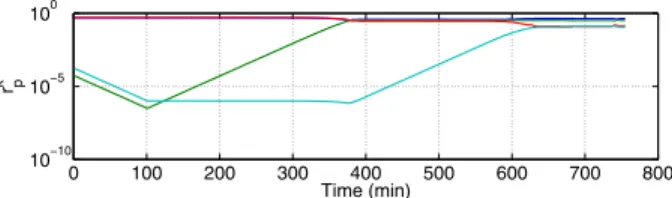
0 100 200 300 400 500 600 700 800 10−10 10−5 100 Time (min) rp k

Fig. 2. Evolution ofrk_pfor the anomalous OD pair (MinDG)

nominal operation. Additionally, and using this set of paths, we compute a routing configuration Rj_robust for every single anomalous traffic event Aj, j ∈ N, where Aj represents a large volume anomaly in traffic from OD pairj. Using a single anomaly detection/localization sequential algorithm, the RRR balances traffic among pathsPkaccording toRjrobustwhen an anomaly of type Aj is detected and localized. This way we avoid to define an uncertainty set that encompasses all possible anomalous traffic. We refer the reader to [17] for details on the implementation of RRR.

B. Improving Dynamic Load Balancing

The DLB algorithms evaluated in Sec. II-C present an important overshoot and a significant settling time in the presence of sudden and large traffic variations. If the traffic anomaly is a perfect step, then the overshoot is unavoidable. We will try to address the long settling time instead. Figure 2 depicts the evolution over time of the correspondingrpkvalues of the anomalous OD pair for MinDG in the example of Sec. II-C. We may see that, although the rkp change exponentially fast, at the moment of the anomaly the values that should increase are so small that it takes them a very long time to converge. A possible solution is to impose a minimum value to allrk_p. However, this will affect the precision of the algorithm and will still result in significant settling times.

Actually, r_pk may be regarded as an indicator of the perfor-mance of path p in the previous iterations. A very small rpk means that p performed very badly with respect to the rest of the paths in the past. However, when the anomaly occurs, conditions severely change and history is no longer as relevant. If we consider that we are in such situation, we could for instance completely ignore history and restart the game by setting r_pk = 1/wk∀k∈Pk. Before deciding how to reassign

rpk, we will discuss how an OD pair may decide if it should restart its game or not.

Consider a situation where most of the traffic for OD pair

k is routed through a path that is not the cheapest, and that ther_pk corresponding to the minimum-cost path is very small. This could mean that although the former performed better in the past, this is no longer true and some traffic should be re-routed to the latter. This is more so as the difference in cost increases. However, this “suspicious” situation could be due to noisy measurements. To make sure that the game have actually changed and that it should be restarted, we will require such a situation to persists during a certain number of consecutive iterations. Once we detected that the game should be restarted, we will re-route some of the traffic that was being

routed through the path with the biggestrk_pto the cheapest one. The amount will be proportional to the relative difference in cost to avoid overreacting. Finally, remember that with WMA fast adaptation is achieved when the r_pk are not too small. The objective with this “game restart” is simply to move rkp from critically small values. The algorithm will then rapidly converge to the optimum. We now present the pseudo-code of the complete algorithm for OD pairk:

Algorithm 2 WMA with Restart (WMA-R) 1: fort= 1, . . . ,∞do

2: Obtain path costsφp ∀p∈Pk

3: Determinepmin=argmin

p∈Pk

φp andpmax=argmax

p∈Pk

rk p 4: if(rk_pmin<0.1)and(φp_min+φth< φp_max)then

5: nk_e←nk_e+ 1 6: else

7: nk_e←0

8: end if

9: ifnk_e≤nk_ththen

10: Perform a normal iteration of WMA (cf. Algorithm 1)

11: else 12: nk_e←0 13: Δr←min φ_φp_pmax min −1,1 ×rpkmax−rkp_min 2 14: r_pk_max←rk_pmax−Δr 15: r_pk_min←r_pk_min+ Δr 16: end if 17: end for

The new variable nk_e counts the number of consecutive occurrences of a “suspicious” situation,. The threshold φth is to make sure that the difference in cost between paths is significant. In particular, we used nk_th = 3, for MinUG we used φth = 0.005 and for MinDG φth = 0.2φpmin. Finally,

note that when the game is restarted, we re-route a certain amount of traffic frompmax topmin, but at most the amount

of traffic routed through each path is equalized. IV. EVALUATION ANDDISCUSSION

In this section we evaluate the performance of the different RR and DLB algorithms presented in this work, considering both normal operation and anomalous traffic situations. We present and discuss three simulation case-scenarios: starting from a normal traffic variation scenario, we increase the number of OD pairs that present anomalous traffic variations. This allows for performance comparison at different levels of traffic variability.

A. Normal Operation

The first case-scenario is the simplest one, which corre-sponds to traffic in normal operation. The only variability is due to typical daily fluctuations. Fig. 3 shows the evolution over time of umax and dmean for the different mechanisms,

when fed with 260 TMs from set X01 in [18]. All algo-rithms perform similarly as regards maximum link utilization, depicted in Fig. 3(a). This may be further appreciated in Fig. 4(a), where we present a boxplot of the difference in

200 400 600 800 1000 1200 0.3 0.35 0.4 0.45 0.5 0.55 Time (min) umax Actual Minimum MinUG MinDG RROP RRAP 200 400 600 800 1000 1200 40 45 50 55 60 65 70 75 Time (min) dmean (kB) Actual Min. MinUG MinDG RROP RRAP

(a) Maximum link utilization (b) Expected e2e queuing delay Fig. 3. Maximum link utilization and expected end-to-end queuing delay under normal operation.

RROP RRAP MinUG MinDG

0 0.05 0.1 0.15 umax (diff)

(a) Maximum link utilization

RROP RRAP MinUG MinDG

1 1.1 1.2 1.3 1.4 dmean ( re la ti ve )

(b) Expected e2e queuing delay Fig. 4. Results overview for the first simulation case-scenario - normal operation.

Naturally, the algorithm that performs best is MinUG, although its improvement over the rest is not significant.

Results with respect to dmean are quiet different, as it can

be seen in Fig. 3(b) and 4(b); the latter shows the dmean

obtained by each mechanism divided by the corresponding actual minimum. We may verify that the best results are obtained by MinDG, followed closely by both RRAP and MinUG. However, RROP systematically obtains a significant difference with respect to the optimum, generally of about 30%. These results further highlight the limitations of RROP as previously discussed in Sec. III-A: using only umax as a

performance objective results in a relatively low maximum utilization, but neglects the rest of the links, impacting global performance. For the case of RRAP, we used α= 0.5 in this and the other case-scenarios.

B. One Anomalous OD Pair

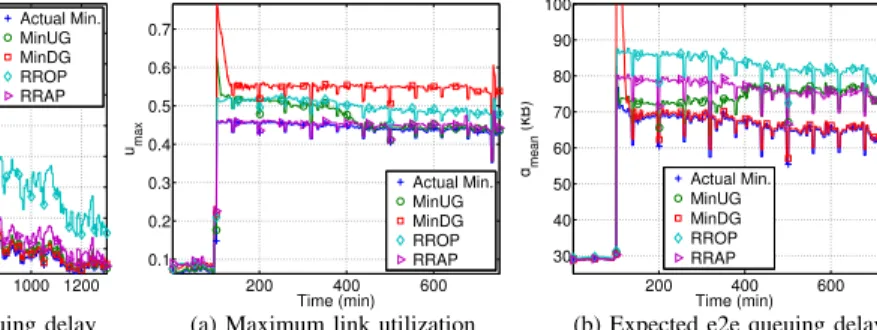
The second case-scenario is the one considered in Sec. II-C, whose main characteristic was the sudden and abrupt increase of traffic generated by one OD pair. Notice in Fig. 5 how the improvements discussed in Sec. III-B for MinUG and MinDG result in a relatively smaller over-shoot than before, but most importantly the settling time has been significantly decreased (cf. Fig. 1).

To be fair with DLB mechanisms, both RRAP and RROP use the RRR mechanism previously described in III-A to adapt traffic balancing after the detection of the anomalous traffic variation. Regarding umax, Fig. 6(a) shows that results

obtained by RRAP are quite good and close to the optimum. Surprisingly enough, the results for RROP are somewhat

200 400 600 0.1 0.2 0.3 0.4 0.5 0.6 0.7 Time (min) umax Actual Min. MinUG MinDG RROP RRAP 200 400 600 30 40 50 60 70 80 90 100 Time (min) dmean (kB) Actual Min. MinUG MinDG RROP RRAP

(a) Maximum link utilization (b) Expected e2e queuing delay Fig. 5. Maximum link utilization and expected end-to-end queuing delay under abrupt and large traffic variations.

RROP RRAP MinUG MinDG

0 0.05 0.1 0.15 0.2 0.25 0.3 umax (diff)

(a) Maximum link utilization

RROP RRAP MinUG MinDG

1 1.1 1.2 1.3 dmean ( re la ti ve )

(b) Expected e2e queuing delay Fig. 6. Results overview for the second simulation case-scenario - abrupt traffic variation.

worse, although the difference is not significant. This differ-ence is probably due to the fact that both RROP and RRAP are solved numerically and not exactly in order to reduce computation time. Results fordmeanfollow the same tendency

as in Sec. IV-A, although both RRAP and MinUG perform somewhat worse than before.

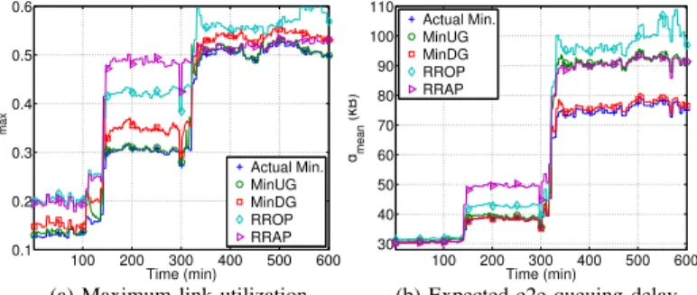
C. Two Anomalous OD Pairs

In this case-scenario two OD pairs largely increase their traffic demand, one at approximately the 150th minute and the other at the 320th. They both present this anomalous traffic until the end of the simulation. We shall then separate the simulation in three parts: the first third where traffic is normal, the second third were only one OD pair is anomalous, and the last third were both OD pairs are anomalous. The anomaly localization algorithm of RRR was designed for the case of one single anomalous OD pair. Because of this, we will further illustrate the tradeoff between size of the considered uncertainty set and efficiency of the obtained routing, and chose the uncertainty polytope by the traffic loads seen after the second anomaly.

In Fig. 7(a) we may see that, as expected, theumaxobtained

by both RROP and RRAP in the last third of the simulation are very close to the optimum. However, in the rest of the simulation the difference may be important, specially in the second part where the difference for RRAP is almost 0.2. It is important to highlight the results obtained by MinDG and MinUG. Notice that the overshoot this time is much smaller than before (a maximum of 0.1 in umax for MinDG) and the

100 200 300 400 500 600 0.1 0.2 0.3 0.4 0.5 0.6 Time (min) umax Actual Min. MinUG MinDG RROP RRAP 100 200 300 400 500 600 30 40 50 60 70 80 90 100 110 Time (min) dmean (kB) Actual Min. MinUG MinDG RROP RRAP

(a) Maximum link utilization (b) Expected e2e queuing delay Fig. 7. Maximum link utilization and expected end-to-end queuing delay under gradual and large traffic variations.

RROP RRAP MinUG MinDG

0 0.05 0.1 0.15 0.2 umax (diff)

(a) Maximum link utilization

RROP RRAP MinUG MinDG

1 1.1 1.2 1.3 1.4 dmean ( re la ti ve )

(b) Expected e2e queuing delay Fig. 8. Results overview for the third simulation case-scenario - gradual traffic variation.

of the anomalous OD pairs is more gradual than before, which clearly favors dynamic schemes in their performance.

V. CONCLUSIONS ANDFUTUREWORK

From the study we performed in this paper we may reach several conclusions. The most important is probably that we have shown that using a single and unique routing configura-tion is not a viable soluconfigura-tion when traffic is relatively dynamic. It obtains a very poor performance either when faced with unforseen TMs or when its design tries to consider as many TMs as possible. It is clear from our study that some form of dynamism is necessary, which could be either RRR (Reactive Robust Routing) or DLB (Dynamic Load-Balancing).

RRR computes a nominal operation routing configuration, and has an alternative routing (using the same paths than in normal operation) for certain possible anomalous situa-tions. In order to detect these anomalous situations, link load measurements have to be gathered. On the other hand, DLB gathers these same measurements but also requires updating load-balancing in a relatively small time-scale. The added complexity is then to distribute these measurements to all ingress routers (instead of a central entity) and updating the load-balancing in real-time.

Our results show that the additional complexity involved in DLB is not justified when the variability (or the anomalies) are not very significant. However, the use of DLB under highly dynamic traffic is very appealing and generally provides better results than RR. Moreover, if the anomalies may not be correctly detected, the only effective solution is DLB.

Regarding RR in particular, a local performance criterium such as umax, widely used in current network optimization problems, does not represent a suitable objective function as regards global network performance. The use ofumaxtogether

with other performance indicator (such as utot) through the

framework of Multi-Objective Optimization provides interest-ing results and deserves further analysis. For instance, we are currently working on the analysis of the Pareto-Optimal solu-tions of the problem, and comparing the resulting performance with that obtained by the AOF approach we presented here.

Dynamic approaches as DLB are generally met with re-luctancy due to their transient behavior under strong traffic variations. However, we have shown that this transient be-havior can be effectively controlled, or at least alleviated, by simple mechanisms. Concerning the two different games we presented, conclusions are similar to those of RR. Minimizing

dmeaninstead ofumaxresults in a somewhat bigger maximum

utilization, but a (sometimes much) better global performance. It should also be highlighted that this paper represents one of the first studies using no-regret algorithms for load-balancing. The results presented here, which were obtained using the most basic of these algorithms, were very promising. There exist other more sophisticated algorithms of this kind, whose exploration we left for future work.

REFERENCES

[1] Cisco-Systems, “Global IP Traffic Forecast and Methodology 2006-2011, white paper”, 2007 - updated 2008, available at http://www.cisco.com.

[2] M. Roughan, M. Thorup and Y. Zhang, “Traffic Engineering with Estimated Traffic Matrices”, inACM IMC ’03, 2003.

[3] C. Zhang, Z. Ge, J. Kurose, Y. Liu and D. Towsley, “On Optimal Routing with Multiple Traffic Matrices”, inIEEE INFOCOM ’05, 2005.

[4] W. Ben-Ameur and H. Kerivin, “Routing of Uncertain Traffic Demands”, in

Optimization and Engineering, vol. 6, pp. 283-313, 2005.

[5] D. Applegate and E. Cohen, “Making Intra-Domain Routing Robust to Changing and Uncertain Traffic Demands: Understanding Fundamental Tradeoffs”, inACM SIGCOMM ’03, 2003.

[6] H. Wang, H. Xie, L. Qiu, Y. Yang, Y. Zhang and A. Greenberg, “COPE: Traffic Engineering in Dynamic Networks”, inACM SIGCOMM ’06, 2006.

[7] A. Elwalid, C. Jin, S. Low and I. Widjaja, “MATE: MPLS Adaptive Traffic Engineering”, inIEEE INFOCOM ’01, 2001.

[8] S. Kandula, D. Katabi, B. Davie and A. Charny, “Walking the Tightrope: Respon-sive yet Stable Traffic Engineering”, inACM SIGCOMM ’05, 2005.

[9] S. Fischer, N. Kammenhuber and A. Feldmann, “REPLEX: dynamic traffic engineering based on wardrop routing policies”, inCoNEXT ’06, 2006. [10] E. Altman, T. Boulogne, R. El-Azouzi, T. Jim´enez and L. Wynter, “A survey on

networking games in telecommunications”,Comput. Oper. Res., vol. 33, no. 2, pp. 286-311, 2006.

[11] F. Larroca and J.L. Rougier, “Routing Games for Traffic Engineering”, inICC ’09. [12] J. Wardrop, “Some theoretical aspects of road traffic research”,Proceedings of the

Institution of Civil Engineers, Part II, vol. 1, no. 36, pp. 352-362, 1952. [13] R. Banner and A. Orda, “Bottleneck Routing Games in Communication Networks”,

IEEE Journal on Selected Areas in Comm., vol. 25, no. 6, pp. 1173-1179, 2007. [14] A. Blum, E. Even-Dar and K. Ligett, “Routing without regret: on convergence to

nash equilibria of regret-minimizing algorithms in routing games”, inPODC ’06. [15] N. Littlestone and M. K. Warmuth, “The weighted majority algorithm”, Inf.

Comput., vol. 108, no. 2, pp. 212-261, 1994.

[16] F. Larroca and J.L. Rougier, “Minimum-Delay Load-Balancing Through Non-Parametric Regression”, inIFIP/TC6 Networking ’09, 2009.

[17] P. Casas, L. Fillatre and S. Vaton, “Robust and Reactive Traffic Engineering for Dynamic Traffic Demands”, inNGI ’08, 2008.

[18] Y. Zhang, “Abilene Dataset 04”, http://www.cs.utexas.edu/∼yzhang/research/ AbileneTM/.