Contents lists available atSciVerse ScienceDirect
Theoretical Computer Science
journal homepage:www.elsevier.com/locate/tcs
Hypervolume-based multiobjective optimization: Theoretical
foundations and practical implications
Anne Auger
a, Johannes Bader
b, Dimo Brockhoff
a,∗, Eckart Zitzler
b aTAO Team INRIA Saclay—Île-de-France, LRI Paris Sud University, 91405 Orsay Cedex, FrancebComputer Engineering and Networks Lab, ETH Zurich, 8092 Zurich, Switzerland
a r t i c l e i n f o Keywords: Multiobjective optimization Evolutionary algorithms Hypervolume indicator Reference point Optimalµ-distributions
a b s t r a c t
In recent years, indicator-based evolutionary algorithms, allowing to implicitly incorporate user preferences into the search, have become widely used in practice to solve multiobjective optimization problems. When using this type of methods, the optimization goal changes from optimizing a set of objective functions simultaneously to the single-objective optimization goal of finding a set of µ points that maximizes the underlying indicator. Understanding the difference between these two optimization goals is fundamental when applying indicator-based algorithms in practice. On the one hand, a characterization of the inherent optimization goal of different indicators allows the user to choose the indicator that meets her preferences. On the other hand, knowledge about the sets ofµpoints with optimal indicator values – the so-calledoptimalµ-distributions– can be used in performance assessment whenever the indicator is used as a performance criterion. However, theoretical studies on indicator-based optimization are sparse.
One of the most popular indicators is the weighted hypervolume indicator. It allows to guide the search towards user-defined objective space regions and at the same time has the property of being a refinement of the Pareto dominance relation with the result that maximizing the indicator results in Pareto-optimal solutions only. In previous work, we theoretically investigated theunweightedhypervolume indicator in terms of a characterization of optimalµ-distributions and the influence of the hypervolume’s reference point for general bi-objective optimization problems. In this paper, we generalize those results to the case of theweightedhypervolume indicator. In particular, we present general investigations for finiteµ, derive a limit result forµgoing to infinity in terms of a density of points and derive lower bounds (possibly infinite) for placing the reference point to guarantee the Pareto front’s extreme points in an optimalµ-distribution. Furthermore, we state conditions about the slope of the front at the extremes such that there is no finite reference point that allows to include the extremes in an optimalµ-distribution— contradicting previous belief that a reference point chosen just above the nadir point or the objective space boundary is sufficient for obtaining the extremes. However, for fronts where there exists a finite reference point allowing to obtain the extremes, we show that forµto infinity, a reference point that is slightly worse in all objectives than the nadir point is a sufficient choice. Last, we apply the theoretical results to problems of the ZDT, DTLZ, and WFG test problem suites.
©2011 Elsevier B.V. All rights reserved.
∗Corresponding address: LIX, École Polytechnique, Palaiseau, France. Tel.: +33 01 69 33 4113.
E-mail addresses:[email protected](A. Auger),[email protected](J. Bader),[email protected](D. Brockhoff),
[email protected](E. Zitzler).
0304-3975/$ – see front matter©2011 Elsevier B.V. All rights reserved.
1. Introduction
Multiobjective optimization aims at optimizing several criteria simultaneously. In the last decades, evolutionary algorithms have been shown to be well-suited for those problems in practice [13,11]. A recent trend is to use quality indicators to turn a multiobjective optimization problem into a single-objective one by optimizing the quality indicator itself. Anindicator-based algorithmuses a specific quality indicator to assign every individual a single-objective fitness—most of the time proportional to theindicator loss, a measure of how much the quality indicator decreases if the corresponding individual is removed from the population. Instead of optimizing the objective functions directly, indicator-based algorithms therefore aim at finding a set of solutions that maximizes the underlying quality indicator and a fundamental question is whether these two optimization goals coincide or how they differ. In practice, the population size of indicator-based algorithms is usually finite, i.e., equal to
µ
∈
N, and the optimization goal changes to finding a set ofµ
solutions optimizing the quality indicator.1We call such a set anoptimalµ
-distribution for the given indicatorgeneralizing the definition given by Auger et al. [2]. In this case, the additional questions arise how the number of pointsµ
influences the optimization goal and to which set ofµ
objective vectors the optimalµ
-distribution is mapped, i.e., which search bias is introduced by changing the optimization goal. Ideally, the optimalµ
-distribution for an indicator only contains Pareto-optimal points and an increase inµ
covers more and more points until the entire Pareto front is covered ifµ
approaches infinity. It is clear that in general, two different quality indicators yield a priori two different optimalµ
-distributions, or in other words, introduce a different search bias. This has for instance been shown experimentally by Friedrich et al. [19] for the multiplicativeε
-indicator and the hypervolume indicator.The hypervolume indicator and its weighted version [33] are particularly interesting indicators since they are refinements of the Pareto dominance relation [37].2Thus, an optimal
µ
-distribution for these indicators contains only Pareto-optimal solutions and the set (probably unbounded in size) that maximizes the (weighted) hypervolume indicator covers the entire Pareto front [18]. Many other quality indicators do not have this fundamental property. It explains the success of the hypervolume indicator as quality indicator applied to environmental selection of indicator-based evolutionary algorithms such as ESP [22], SMS-EMOA [5], MO-CMA-ES [24], or HypE [3]. Nevertheless, it has been argued that using the (weighted) hypervolume indicator to guide the search introduces a certain bias. Interestingly, several contradicting beliefs about this bias have been reported in the literature which we will discuss later on in more detail (see Section3). They range from stating thatconvex regions may be preferred to concave regionsto the argumentation thatthe hypervolume is biased towards boundary solutions. In the light of those contradicting beliefs, a thorough investigation of the effect of the hypervolume indicator on optimalµ
-distributions is necessary.Another important issue when dealing with the hypervolume indicator is the choice of the reference point, a parameter, both the unweighted and the weighted hypervolume indicator depend on. The influence of this reference point on optimal
µ
-distributions has not been fully understood, especially for the weighted hypervolume indicator, and only rules-of-thumb exist on how to choose the reference point in practice. In particular, it could not be observed from practical investigations how the reference point has to be set to ensure to find the extremes of the Pareto front. Several authors recommend to use the corner of a space that is a little bit larger than the actual objective space as the reference point [26,5]. For performance assessment, others recommend to use the estimated nadir point as the reference point [32,31,23]. Also here, theoretical investigations are highly needed to assist in practical applications.First theoretical studies on optimal
µ
-distributions for the (unweighted) hypervolume indicator and the choice of its reference point have been published in an earlier work by the authors [2]. The theoretical analyses resulted in a better understanding of the search bias the hypervolume indicator introduces and in theoretically founded recommendations on where to place the reference point in the case of two objectives. In particular, some beliefs about the indicator’s search bias could be disproved and others confirmed, the optimalµ
-distributions for linear Pareto fronts were characterized exactly (see also [10]), and lower bounds on the reference point’s objective values that allow to include the extremes of the Pareto front in certain cases have been given. Recently, a specific result of Auger et al. [2] has been already generalized to the weighted hypervolume indicator [1] and another exact result for specific Pareto fronts have been provided [19].In this paper, we extend all results by Auger et al. [2] to the weighted case and provide a general theory of the weighted hypervolume indicator in terms of both the inherently introduced search bias and the choice of the reference point.
•
In particular, we characterize the sets ofµ
points that maximize the (weighted) hypervolume indicator; besides general investigations for finiteµ
, we derive a limit result forµ
going to infinity in terms of a density of points. The presented results for the weighted hypervolume indicator comply with the results for the unweighted case [2].•
Furthermore, we investigate the influence of the reference point on optimalµ
-distributions, i.e., we derive lower bounds for the objective values of the reference point (possibly infinite) for guaranteeing the Pareto front’s extreme points in an optimalµ
-distribution and investigate cases where the extremes are never contained in such a set; these results generalize the work by Auger et al. [2] to the weighted hypervolume indicator.1 Sometimes, the population size might not be fixed, e.g., when deleting all dominated solutions, but the maximum number of simultaneously considered solutions is typically upper bounded by a constantµ.
•
In addition, we prove, in case the extremes can be obtained, that for any reference point dominated by the nadir point – with any small but positive distance between the two points – there is a finite number of pointsµ
0(possibly large in practice) such that for allµ > µ
0, the extremes are included in optimalµ
-distributions.•
Last, we apply the theoretical results to linear Pareto fronts [2,10] and to benchmark problems of the ZDT [34], DTLZ [15], and WFG [21] test problem suites resulting in recommended choices of the reference point including numerical and sometimes analytical expressions for the resulting density of points on the front.The paper is structured as follows. First, we recapitulate the basics of the (weighted) hypervolume indicator and introduce the notations and definitions needed in the remainder of the paper (Section2). Then, we consider the bias of the weighted hypervolume indicator in terms of optimal
µ
-distributions. After characterizing optimalµ
-distributions for a finite number of solutions (Section3.1), we derive results on the density of points if the number of points goes to infinity (Section3.2). Section4investigates the influence of the reference point on optimalµ
-distributions especially on the extremes. The application of the results to test problems is presented in Section5, and Section6concludes the paper.2. The hypervolume indicator: general aspects and notations
Throughout this study we consider, without loss of generality, minimization problems wherekobjective functions Fi
:
X→
Z, 1≤
i≤
khave to be minimized simultaneously. The vector functionF:=
(
F1, . . . ,
Fk)thereby maps each solutionxin the decision spaceXto its corresponding objective vectorF(
x)
in the objective spaceF(
X)
=
Z⊆
Rk. Furthermore, we assume that the underlying dominance structure is given by the weak Pareto dominance relation≼
which is defined between arbitrary solution pairs. We sayx∈
X weakly dominates y∈
Xif for all 1≤
i≤
k,Fi(
x)
≤
Fi(y)
and write x≼
y. This weak Pareto dominance relation is generalized to sets of solutions in the following straightforward manner: we say a setAof solutions weakly dominates another solution setBif for allb∈
Bthere exists ana∈
Asuch thata≼
b. The Pareto(-optimal) set Psconsists of all solutionsx∗∈
X, such that there is nox∈
Xthat satisfiesx≼
x∗andx∗̸≼
x. The image ofPsunderF is calledPareto(-optimal) frontorfrontfor short. We also use the weak Pareto dominance relation notation≼
among objective vectors, i.e., for two objective vectorsx=
(
x1, . . . ,
xk),y=
(
y1, . . . ,
yk)∈
Rkwe definex≼
yif and only if for all 1≤
i≤
k:
xi≤
yi.In the following, in order to simplify notations,3we define the indicators forsets of objective vectors A
⊆
Rkinstead for solution sets A′⊆
Xas it was already done before [33,2]. The weighted hypervolume indicatorIH,w(A,
r)
for a set of objective vectorsA⊆
Zis then the weighted Lebesgue measure of the set of objective vectors weakly dominated by the solutions in Athat at the same time weakly dominate a so-called reference pointr∈
Z[3]4:IH,w(A
,
r)
=
Rk
w(
z)
1H(A,r)(z)
dz (1)whereH
(
A,
r)
:= {
z∈
Z| ∃
a∈
A:
a≼
z≼
r}
,1H(A,r)(z)
is the characteristic function ofH(
A,
r)
that equals 1 iff z∈
H(
A,
r)
and 0 otherwise, andw
:
Rk→
R>0is a strictly positive weight function integrable on any bounded set, i.e.,
B(0,γ )
w(
z)
dz<
∞
for anyγ >
0, whereB(
0, γ )
is the open ball centered in 0 and of radiusγ
. In other words, we assume that the measure associated tow
isσ
-finite.5Throughout the paper, the notationIHrefers to the non-weighted hypervolume where the weight is 1 everywhere, and we will explicitly use the term non-weighted hypervolume forIHwhile the weighted hypervolume indicatorIH,wis, for simplicity, referred to as hypervolume.
The left-hand plot ofFig. 1illustrates the hypervolumeIH,wfor a bi-objective problem. The three-objective plot shows the objective values of nine points on the first two axes and the weight function
w
on the third axis. The hypervolume indicatorIH,w(A)
for the setAof nine points equals the integral of the weight function over the objective space that is weakly dominated by the setAand which weakly dominates the reference pointr=
(
r1,
r2)
.In what follows, we consider bi-objective problems. The Pareto front can thus be described by a one-dimensional function f mapping the image of the Pareto set under the first objectiveF1 onto the image of the Pareto set under the second objectiveF2,
f
:
x∈
D→
f(
x),
whereDdenotes the image of the Pareto set under the first objective.Dcan be, for the moment, either a finite or an infinite set. An illustration is given in the right-hand plot ofFig. 1where the functionf describing the front has a domain of D
= [
xmin,
xmax]
.3 Considering an indicator on solution sets introduces the possibility of solutions that map to the same objective vector. Adding such a so-calledindifferent solutionto a solution set does not affect the set’s hypervolume indicator value but the consideration of such solutions makes the text less readable if we want to state the results formally correct.
4 Instead of a reference set as by Bader and Zitzler [3], we consider one reference point only as in earlier publications [33].
5 Several results presented in this paper also hold if the weight is strictly positive almost everywhere, i.e., it can be 0 for null sets. However, we decided to consider only strictly positive weights to keep the proofs simple.
Fig. 1.The hypervolume indicatorIH,w(A)corresponds to the integral of a weight functionw(z)over the set of objective vectors that are weakly dominated by a solution setAand in addition weakly dominate the reference pointr(hatched areas). On the left, the setAconsists of nine objective vectors whereas on the right, the infinite setAcan be described by a functionf: [xmin,xmax] →R. The left-hand plot shows an example of a weight functionw(z), where for all objective vectorszthat are not dominated byAor not enclosed byrthe functionwis not plotted, such that the weighted hypervolume indicator corresponds to the volume of the gray shape.
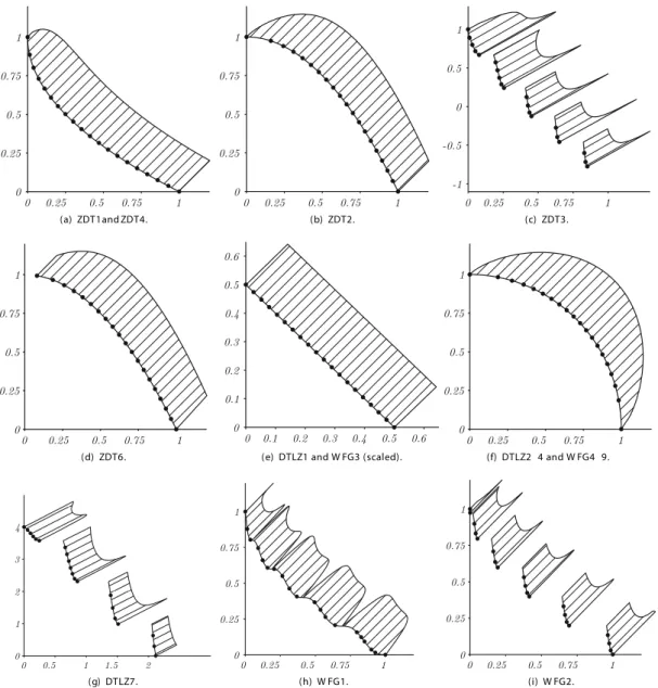
Example 1. Consider the bi-objective problem DTLZ2 [15] which is defined as minimize F1
(
d)
=
1+
g(
dM)
cos(
d1π/
2)
minimize F2(
d)
=
1+
g(
dM)
sin(
d1π/
2)
g(
dM)
=
di∈dM(
di−
0.
5)
2 subject to 0≤
di≤
1 fori=
1, . . .
n (2)wheredMdenotes a subset of the decision variablesd
=
(
d1, . . . ,
dn)∈ [
0,
1]
nwithg(
dM)≥
0. The Pareto front is reached forg(
dM)=
0. Hence, the Pareto-optimal points have objective vectors(
cos(
d1π/
2),
sin(
d1π/
2))
with 0≤
d1≤
1 which can be rewritten as points(
x,
f(
x))
withf(
x)
=
√
1
−
x2andx∈
D= [
0,
1]
; seeFig. 9(f).Sincef represents the shape of the trade-off surface, we can conclude that, for minimization problems,f is strictly monotonically decreasing inD.6The coordinates of a point belonging to the Pareto front are given as a pair
(
x,
f(
x))
with x∈
Dand therefore, a point is entirely determined by the functionf and the first coordinatex∈
D. Forµ
points on the Pareto front, we denote their first coordinates as(
x1, . . . ,
xµ). Without loss of generality, it is assumed thatxi≤
xi+1, for i=
1, . . . , µ
−
1 and for notation convenience, we setxµ+1:=
r1andf(
x0)
:=
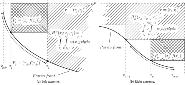
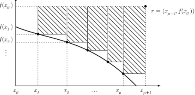
r2wherer1andr2are the first and second coordinate of the reference point (seeFig. 2). The weighted hypervolume enclosed by these points can be decomposed intoµ
components, each corresponding to the integral of the weight functionw
over a rectangular area (seeFig. 2). The resulting weighted hypervolume writes:IH,w((x1
, . . . ,
xµ)):=
µ
i=1
xi+1 xi
f(x0) f(xi)w(
x,
y)
dy
dx.
(3)When the weight function equals one everywhere, one retrieves the expression for the (non-weighted) hypervolume [2] IH
((
x1, . . . ,
xµ)):=
µ
i=1
(
xi+1−
xi)(f(
x0)
−
f(
xi)). (4)Indicator-based evolutionary algorithms that aim at optimizing a unary indicatorI
:
2X→
Rsuch as the hypervolume transform a multiobjective problem into the single-objective one consisting of finding a set of points maximizing the respective indicatorI. In practice, the cardinality of these sets of points is usually upper bounded by a constantµ
, typically the population size. Generalizing the definition by Auger et al. [2], we define anoptimalµ
-distributionas a set ofµ
points maximizingI.Definition 1 (Optimal
µ
-Distribution). Forµ
∈
Nand a unary indicatorI, a set ofµ
points maximizingIis called an optimalµ
-distribution forI.The rest of the paper is devoted to understand optimal
µ
-distributions for the hypervolume indicator in the bi-objective case. Thex-coordinates of an optimalµ
-distribution for the hypervolumeIH,wwill be denoted(
xµ1, . . . ,
xµµ)
and will thus satisfyIH,w((xµ1
, . . . ,
xµµ))
≥
IH,w((x1, . . . ,
xµ)) for all(
x1, . . . ,
xµ)∈
D× · · · ×
D.
6 Iffis not strictly monotonically decreasing, we can find Pareto-optimal points(x1,f(x1))and(x2,f(x2))withx1,x2∈Dsuch that, without loss of generality,x1<x2andf(x1)≤f(x2), i.e.,(x1,f(x1))dominates(x2,f(x2)).
Fig. 2.Computation of the hypervolume indicator forµsolutions(x1,f(x1)), . . . , (xµ,f(xµ))and the reference pointr=(r1,r2)in the bi-objective case as defined in Eqs. (3) and (4) respectively.
Note, that the optimal
µ
-distribution might not be unique, and(
xµ1, . . . ,
xµµ)
therefore refers tooneoptimalµ
-distribution. The corresponding value of the hypervolume will be denotedIH,wµ , i.e.,IH,wµ=
IH,w((xµ1, . . . ,
xµµ))
.Remark 1. Looking at Eqs. (3) and (4), we see that for a fixedf, a fixed weight
w
, and a fixed reference point, the problem of finding a set ofµ
points maximizing the weighted hypervolume amounts to finding the solution of aµ
-dimensional single-objective maximization problem, i.e., optimalµ
-distributions are the solution of a single-objective problem ofµ
variables.3. Characterization of optimal
µ
-distributions for hypervolume indicatorsSeveral contradicting beliefs about the bias introduced by the hypervolume indicator have been reported in the literature. For example, Zitzler and Thiele [36] stated that, when optimizing the hypervolume in maximization problems, ‘‘convex regions may be preferred to concave regions’’, which has been also stated by Lizarraga-Lizarraga et al. [30] later on, whereas Deb et al. [14] argued that ‘‘[. . . ] the hypervolume measure is biased towards the boundary solutions’’. Knowles and Corne [28] observed that a local optimum of the hypervolume indicator ‘‘seems to be ‘well-distributed’’’ which was also confirmed empirically [29,16]. Beume et al. [5], in addition, state several properties of the hypervolume’s bias: (i) optimizing the hypervolume indicator focuses on knee points; (ii) the distribution of points on the extremes is less dense than on knee points; (iii) only linear front shapes allow for equally spread solutions; and (iv) extremal solutions are maintained. In the light of these contradicting statements, a thorough characterization of optimal
µ
-distributions for the hypervolume indicator is necessary. Especially for the weighted hypervolume indicator, the bias of the indicator and the influence of the weight functionw
on optimalµ
-distributions in particular has not been fully understood.In this section, we first prove the existence of optimal
µ
-distributions for lower semi-continuous fronts, we show the monotonicity inµ
of the hypervolume associated with optimalµ
-distributions, and derive necessary conditions satisfied by optimalµ
-distributions. In a second part, we derive the density associated with optimalµ
-distributions whenµ
grows to infinity.3.1. Finite number of points
3.1.1. Existence of optimal
µ
-distributionsBefore to further investigate optimal
µ
-distributions forIH,w, we establish a setting ensuring their existence. We will from now on assume thatDis a closed interval that we denote[
xmin,
xmax]
such thatfwrites:x
∈ [
xmin,
xmax] →
f(
x).
A function is lower semi-continuous if for allx0, lim infx→x0f
(
x)
≥
f(
x0)
. Iffis decreasing (which is the case whenfdescribes a Pareto front), lower semi-continuous is equivalent to continuity to the right. As shown in the following theorem, a sufficient setting for the existence of optimal distributions is the lower semi-continuity off.Theorem 1 (Existence of Optimal
µ
-Distributions). Letµ
∈
N, if the function f describing the Pareto front is lower semi-continuous, there exists (at least) one set ofµ
points maximizing the hypervolume.Proof. We are going to prove thatIH,wis upper semi-continuous iffis lower semi-continuous, and then apply the Extreme Value Theorem. SinceIH,wis the sum of
µ
functionsg(
xi,xi+1)
whereg(α, β)
=
βα
(
f(x0)f(α)
w(
x,
y)
dy)
dx, we will prove the upper semi-continuity ofg(
xi,xi+1)
for(
xi,
xi+1)
∈ [
xmin,
xmax]
. This will imply the upper semi-continuity ofIH,w[7, p. 362]. Let(
xi,
xi+1)
∈ [
xmin,
xmax]
and let(
xni,
xni+1)n
∈N converging to(
xi,xi+1)
. We will now prove that lim supg(
xni,
xni+1)
≤
g(
xi,xi+1)
(see [25], p. 481). Since lim sup n→∞ g(
xni,
xni+1)
=
lim sup n→∞
1[xni,xni+1](
x)
1[f(xni),f(x0)](
y)w(
x,
y)
dydx,
and 1[xni,xni+1]
(
x)
1[f(xi),f(x0)](
x)w(
x,
y)
≤
1[xmin,xmax](
x)
1[f(xmax),f(x0)](
x)w(
x,
y)
we can use the (Reverse) Fatou Lemma [25, p. 252] that implies lim supg(
xni,
xni+1)
≤
lim sup1[xni,xni+1](
x)
1[f(xni),f(x0)](
y)w(
x,
y)
dydx.
Sincef is lower semi-conti-nuous, lim inff(
xni)
≥
f(
xi)holds which is equivalent to lim sup(
f(
x0)
−
f(
xni))
=
f(
x0)
−
lim inff(
xni)
≤
f(
x0)
−
f(
xi). Hence, lim sup1[f(xni),f(x0)](
y)
≤
1[f(xi),f(x0)](
y)
and thuslim sup n→∞
g
(
xni,
xni+1)
≤
1[xi,xi+1]
(
x)
1[f(xi),f(x0)](
y)w(
x,
y)
dydx=
g(
xi,xi+1).
We have proven the upper semi-continuity ofgwhich implies the upper semi-continuity ofIH,w
: [
xmin,
xmax]
µ→
R. Given that[
xmin,
xmax]
µis compact, we can imply from the Extreme Value Theorem that there exists a set ofµ
points maximizing the hypervolume indicator.Note that, in case of bi-objectivemaximizationproblems, the lower semi-continuity off has to be changed into upper semi-continuity which has been proven recently for the unweighted hypervolume [9]. Note also that the previous theorem states the existence but not the uniqueness, which cannot be guaranteed in general. With this respect, we would like to mention that the question of uniqueness is related loosely to another property of the hypervolume which is not discussed here but has high importance in practice: for indicator-based algorithms and the analysis of their convergence speed, it is highly important whetherlocaloptima are observed during the search. This property is, however, defined within the decision spaceXand especially depends on the mapping between the decision space and the objective space which is not taken into account in this study.
Furthermore, if the front is not semi-continuous, optimal
µ
-distributions might not exist. In the following proposition, we construct an example of a front where this is the case, i.e., where there isnooptimalµ
-distribution forµ
=
1.Proposition 1. Let r
=
(
r1,
r1)
be a reference point with r1>
1.
2. Consider the front fce: [
0,
1] → [
0,
1.
2]
with fce(
x)
=
1−
x+
0.
2 if x≤
1 2,
1−
x if x∈ ]
1 2,
1]
.
Then f does not admit an optimal1-distribution for the unweighted hypervolume.
Proof. Consider first the linear frontf
:
x∈ [
0,
1] → [
0,
1]
,
x→
1−
x. Here, the optimal 1-distribution is the point(
0.
5,
0.
5)
with a corresponding hypervolume value ofγ
=
(
r1−
12)(
r1−
12)
.7Consider nowh(
x)
=
fce(
x)
for allx∈ [
0,
1]
except forx=
0.
5 whereh(
x)
=
0.
5. Then,his continuous to the right and thus lower semi-continuous. Hence, according toTheorem 1it admits an optimal 1-distribution. In addition, remark that the hypervolume contribution for anyx
∈ [
0,
0.
5[
is strictly smaller forhthan forf and equal forx
∈ [
0.
5,
1]
. Thus(
0.
5,
0.
5)
is also the optimal 1-distribution ofhwith hypervolumeγ
. However, forfce, the hypervolume contribution is strictly smaller than forf forx∈ [
0,
0.
5]
and equal for x∈ ]
0.
5,
1]
with a gap at 0.
5 such thatγ
cannot be reached for any point in[
0,
1]
though one has values arbitrary close from it forxarbitrary close from 0.
5 to the right.We have chosen
µ
=
1 in the previous proposition for the sake of simplicity, however, such a counter-example can be generalized for arbitraryµ
by following the same idea. Let us also note that, lower semi-continuity is not a necessary condition for the existence of optimalµ
-distributions: if we simply introduce the discontinuity of the functionfcein the previous proposition somewhere in]
0,
0.
5[
instead of atx=
0.
5, the optimal 1-distribution would exist (and be located at x=
0.
5) though the function describing the front is not lower semi-continuous.3.1.2. Strict monotonicity of hypervolume in
µ
for optimalµ
-distributionsThe following proposition establishes that the hypervolume of optimal
(µ
+
1)
-distributions is strictly larger than the hypervolume of optimalµ
-distributions. This result is a generalization of Auger et al. [2, Lemma 1].Proposition 2. Let D
⊆
R, possibly finite and f:
x∈
D→
f(
x)
describe a Pareto front. Letµ
1andµ
2∈
Nwithµ
1< µ
2, then Iµ1H,w
<
IH,wµ2holds if D contains at least
µ
1+
1elements xifor which xi<
r1and f(
xi) <r2holds.Proof. To prove the proposition, it suffices to show the inequality for
µ
2=
µ
1+
1. AssumeDµ1= {
x µ11
, . . . ,
x µ1 µ1}
withxµi
∈
Ris the set ofx-values of the objective vectors of the optimalµ
1-distribution forIH,wwith a hypervolume value of Iµ1H,wif the Pareto front is described byf. SinceDcontains at least
µ
1+
1 elements, the setD\
Dµ1 is not empty and we can pick anyxnew∈
D\
Dµ1that is not contained in the optimalµ
1-distribution forIH,wand for whichf(
xnew)
is defined. Letxr
:=
min{
x|
x∈
Dµ1∪{
r1}
,
x>
xnew}
be the closest element ofDµ1to the right ofxnew(orr1ifxnewis larger than all elements ofDµ1). Similarly, letfl:=
min{
r2,
{
f(
x)
|
x∈
Dµ1,
x<
xnew}}
be the function value of the closest element ofDµ1to the left of7 In caseµ=1 andf(x)=1−x, we can easily compute the maximum of the hypervolumeIH,w(x)=(r1−x)(r1−(1−x))=r12−r1+x−x2of the single point atxby computing the derivative ofIH,w(x)and setting it to zero:IH′,w(x)=1−2x=0.
xnew(orr2ifxnewis smaller than all elements ofDµ1). Then, all objective vectors withinHnew
:= [
xnew,
xr[ × [
f(
xnew),
fl[
are weakly dominated by the new point(
xnew,
f(
xnew))
but are not dominated by any objective vector given byDµ1. Furthermore,Hnewis not a null set (i.e., has a strictly positive measure) sincexnew
>
xrandfl>
f(
xnew)
and the weightw
is strictly positive which givesIµ1H,w
<
IH,wµ2 .3.1.3. Characterization of optimal
µ
-distributions for finiteµ
In this section, we derive a general result to characterize optimal
µ
-distributions for the hypervolume indicator ifµ
is finite. The result holds under the assumption that the frontf is differentiable and is a direct application of the fact that solutions of a maximization problem that do not lie on the boundary of the search domain are stationary points, i.e., points where the gradient is zero.Theorem 2 (Necessary Conditions for Optimal
µ
-distributions for IH,w). If f is continuous and differentiable and(
xµ1, . . . ,
xµµ)
are the x-coordinates of an optimalµ
-distribution for IH,w, then for all xµi with xiµ>
xminand xµi<
xmaxf′
(
xµi)
xµi+1 xµiw(
x,
f(
xµi))
dx=
f(xµi) f(xµi−1)w(
xµi,
y)
dy (5)holds where f′denotes the derivative of f , f
(
xµ0)
=
r2and xµµ+1=
r1.Proof. The proof idea is simple: optimal
µ
-distributions maximize theµ
-dimensional functionIH,wdefined in Eq. (3) and should therefore satisfy necessary conditions for local extrema of aµ
-dimensional function stating that the coordinates of local extrema either lie on the boundary of the domain (herexminorxmax) or satisfy that the partial derivative with respect to this coordinate is zero. Hence, we see that the partial derivatives ofIH,whave to be computed. This step is quite technical and is presented inAppendix A.1on page92together with the full proof of the theorem.The previous theorem proves an implicit relation between the points of an optimal
µ
-distribution. However, in certain cases of weights, this implicit relation can be made explicit as illustrated first on the example of the weight functionw(
x,
y)
=
exp(
−
x)
, aiming at favoring points with small values along the first objective.Example 2. If
w(
x,
y)
=
exp(
−
x)
, Eq. (5) simplifies into the explicit relation f′(
xµi)(
e−xµi−
e−x µ i+1)
=
e−xµi(
f(
xµ i)
−
f(
x µ i−1)).
(6)Another example where the relation is explicit is given for the unweighted hypervolumeIH that we can obtain as a corollary of the previous theorem and which coincides with a previous result [2, Proposition 1].
Corollary 1 (Necessary Condition for Optimal
µ
-Distributions for IH). If f is continuous, differentiable and(
xµ1, . . . ,
xµµ)
are the x-coordinates of an optimalµ
-distribution for IH, then for all xµi with xµ
i
>
xminand xµi<
xmax f′(
xµi)(
xµi+1−
x µ i)
=
f(
x µ i)
−
f(
x µ i−1)
(7)holds where f′denotes the derivative of f , f
(
xµ0
)
=
r2and xµµ+1=
r1.Proof. The proof follows immediately from setting
w
=
1 in Eq. (5).Remark 2. Corollary 1implies that the points of an optimal
µ
-distribution forIHare linked by a second order recurrence relation. Thus, in this case, finding optimalµ
-distributions for IH does not correspond to solving aµ
-dimensional optimization problem as stated inRemark 1but to a two-dimensional one. The same remark holds forIH,wandw(
x,
y)
=
exp
(
−
x)
as can be seen in Eq. (6).The previous corollary can also be used to characterize optimal
µ
-distributions for certain Pareto fronts more generally as the following example shows.Example 3. Consider a linear Pareto front, i.e., a front that can be formally defined asf
:
x∈ [
xmin,
xmax] →
α
x+
β
whereα <
0 andβ
∈
R. Then, it follows immediately fromCorollary 1and Eq. (7) that the optimalµ
-distribution forIHmaps to objective vectors with equal distances between two neighbored solutions (see alsoTheorem 7in Section5.1):α
xµi+1−
x µ i
=
f(
xµi)
−
f(
xµi−1)
=
α(
x µ i−
x µ i−1)
fori
=
2, . . . , µ
−
1. Note that this result coincides with earlier results for linear fronts with slopeα
= −
1 [4] or the even more specific case of a front of shapef(
x)
=
1−
x[17].3.2. Number of points going to infinity
Besides for simple fronts, like the linear one, Eq. (5) and Eq. (7) cannot be easily exploited to derive optimal
µ
-distributions explicitly. However, one is interested in knowing how the hypervolume indicator influences the spread of points on the frontFig. 3.Every continuous frontg(x)(left) can be described by a functionf:x′∈ [
0,x′ max] →f(x
′)
withf(x′
max)=0 (right) by a simple translation.
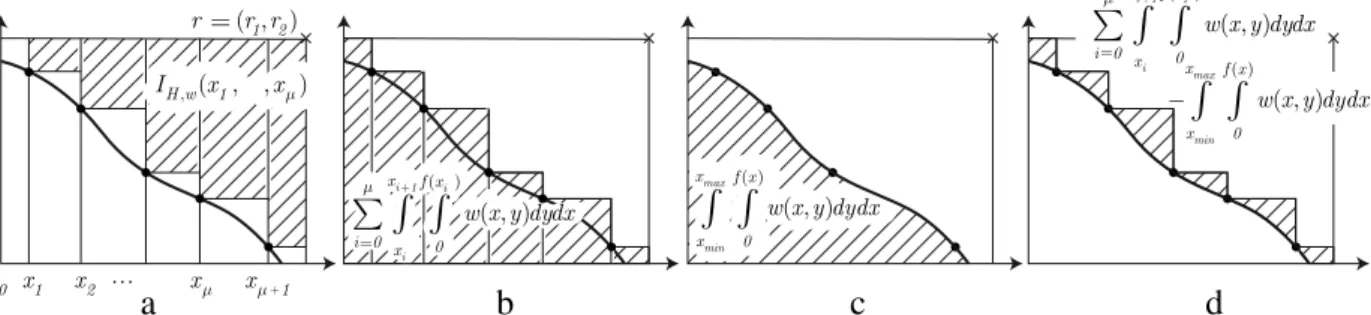
Fig. 4.Illustration of the idea behind deriving the optimal density: Instead of maximizing the weighted hypervolume indicatorIH,w((x1, . . . ,xµ))(a), one can minimize the shaded area in (b) which is equivalent to minimizing the integral between the attainment surface of the solution set and the front itself which can be expressed with the help of the integral off(d).
and in characterizing the bias introduced by the hypervolume. To reply to these questions, we will assume that the number of points
µ
grows to infinity and derive the density of points associated with optimalµ
-distributions for the hypervolume indicator.We assume without loss of generality thatxmin
=
0 and thatf:
x∈ [
0,
xmax] →
f(
x)
withf(
xmax)
=
0 (Fig. 3). We also assume thatf is continuous within[
0,
xmax]
, differentiable, and that its derivative is a continuous functionf′defined in the interval]
0,
xmax[
. Instead of maximizing the weighted hypervolume indicatorIH,w, it is easy to see that, sincer1r2is constant, one can equivalently minimizer1r2
−
IH,w((x1, . . . ,
xµ))=
µ
i=0
xi+1 xi
f(xi) 0w(
x,
y)
dydxwithx0
=
0,f(
x0)
=
r2, andxµ+1=
r1(seeFig. 4(b)). If we subtract the area below the front curve, i.e., the integral
xmax0
(
f(x)0
w(
x,
y)
dy)
dxof constant value (Fig. 4(c)), we see that minimizing µ
i=0
xi+1 xi
f(xi) 0w(
x,
y)
dydx−
xmax 0
f(x) 0w(
x,
y)
dydx (8)is equivalent to maximizing the weighted hypervolume indicator (Fig. 4(d)).
For a fixed integer
µ
, we now consider a sequence ofµ
ordered pointsxµ1, . . . ,
xµµin[
0,
xmax]
that lie on the Pareto front. We assume that the sequence converges – whenµ
goes to∞
– to a densityδ(
x)
that is regular enough. Formally, the density inx∈ [
0,
xmax]
is defined as the limit of the number of points contained in a small interval[
x,
x+
h[
normalized by the total number of pointsµ
when bothµ
goes to∞
andhto 0, i.e.,δ(
x)
=
limµ→∞h→0
(
1 µh
µi=11[x,x+h[
(
xµi))
. As explained above,maximizing the weighted hypervolume is equivalent to minimizing Eq. (8), which is also equivalent to minimizing Eµ
=
µ
µ
i=0
xµi+1 xµi
f(xµi) 0w(
x,
y)
dy
dx−
xmax 0
f(x) 0w(
x,
y)
dy
dx
,
(9)where we have multiplied Eq. (8) by
µ
to obtain a quantity that will converge to a limit whenµ
goes to∞
. Indeed Eq. (8) converges to 0 whenµ
increases. We now conjecture that the equivalence between minimizingEµand maximizing the hypervolume also holds forµ
going to infinity. Therefore, our proof consists of two steps: (1) compute the limit ofEµwhenµ
goes to∞
. This limit is going to be a function of a densityδ
. (2) Find the densityδ
that minimizesE(δ)
:=
limµ→∞Eµ.Lemma 1. If f is continuous, differentiable with the derivative f′continuous, if x
→
w(
x,
f(
x))
is continuous, if xµ1, . . . ,
xµµ converge to a continuous densityδ
, with1δ∈
L2(
0,
xmax
)
,8and∃
c∈
R+such thatµ
sup
sup 0≤i≤µ−1|
xµi+1−
x µ i|
,
|
xmax−
xµµ|
→
cthen Eµconverges for
µ
→ ∞
to E(δ)
:= −
1 2
xmax 0 f′(
x)w(
x,
f(
x))
δ(
x)
dx.
(10)Proof. For the technical proof, we refer toAppendix A.2on page94.
The limit density of a
µ
-distribution forIH,w, as explained before, minimizesE(δ)
. It remains therefore to find the density which minimizesE(δ)
. This optimization problem is posed in a functional space and is also a constrained problem since the densityδ
has to satisfy the constraintJ(δ)
:=
xmax0
δ(
x)
dx=
1. The constraint optimization problem (P) that needs to be solved is summarized in:minimizeE
(δ)
subject toJ
(δ)
=
1.
(P)In a similar way than Theorem 7 in [2] where
−
f′needs to be replaced everywhere by−
f′w
,9we find that the density solution of the constraint optimization problem (P) equalsδ(
x)
=
√
−
f′(
x)w(
x,
f(
x))
xmax 0√
−
f′(
x)w(
x,
f(
x))
dx.
Forxmin
̸=
0, the density readsδ(
x)
=
√
−
f′(
x)w(
x,
f(
x))
xmax xmin√
−
f′(
x)w(
x,
f(
x))
dx.
(11)Remark 3. The previous density corresponds to the density of points of the front projected onto the x-axis, however, if one is interested into the density on the front
δF
10one has to normalize the result from Eq. (11) by the norm of the tangent for points of the front, i.e.,
1+
f′(
x)
2. Therefore, the density on the front isδF
(
x)
=
√
−
f′(
x)w(
x,
f(
x))
xmax xmin√
−
f′(
x)w(
x,
f(
x))
dx 1
1+
f′(
x)
2.
(12)Example 4. Let us consider the test problem ZDT2 [34, see alsoFig. 9] the Pareto front of which can be described by f
(
x)
=
1−
x2withxmin
=
0 andxmax=
1 andf′(
x)
= −
2x[2]. Considering the unweighted case, the density on the x-axis according to Eq. (11) isδ(
x)
=
32
√
xand the density on the front according to Eq. (12) is
δF
(
x)
=
32 √ x
√
1+4x2; seeFig. 9 for an illustration.To summarize, we have seen that the density follows as a limit result from the fact that the integral between the attainment function of the solution set with
µ
points and the front itself (Fig. 4(d)) has to be minimized and the optimalµ
-distribution forIH,wand a finite number of points converges to the density whenµ
increases. Furthermore, we can conclude that the proportion of points of an optimalµ
-distribution withx-values within a certain interval[
a,
b]
converges to
ba
δ(
x)
dxif the number of pointsµ
goes to infinity. How this relates to practice will be presented in Section5where analytical and experimental results on the density for specific well-known test problems are shown.Instead of applying the results to specific test functions, the above results on the hypervolume indicator can also be interpreted in a broader sense: from Eq. (11), we know that it is only the weight function and the slope of the front that influences the density of the points of an optimal
µ
-distribution—contrary to several prevalent beliefs as stated in the beginning of this section. Since the density of points does not depend on the position on the front but only on the gradient and the weight at the respective point, the density close to the extreme points of the front can be very high or very low—it only depends on the front shape. Section4.1.1will even present conditions under which the extreme points will never be8L2(0,x
max)is a functional space (Banach space) defined as the set of all functions whose square is integrable in the sense of the Lebesgue measure. 9 Note that in [2, Theorem 7] and its proof, the density should belong toL2(0,x
max)but also, 1/δ∈L2(0,xmax).
10 The density on the front gives for any curve on the front (a piece of the front) C, the proportion of points of the optimalµ-distribution (forµto infinity) contained in this curve by integration on the curve
CδFds. Since we know that for any parametrization of C, sayt ∈ [a,b] → γ (t) ∈ R2, we have
CδFds= b
aδF(γ (t))∥γ′(t)∥2dt, we can for instance use the natural parametrization of the front given byγ (t)=(t,f(t))giving∥γ′(t)∥2=
1+f′(t)2 that therefore implies thatδ(x)=δF(x)
1+f′(x)2. Note that we do a small abuse of notation writingδ
included in an optimal
µ
-distribution forIH,w—in contrast to the statement by Beume et al. [5]. In the unweighted case, we observe that the density has its maximum for front parts where the tangent has a gradient of−
45◦[see also2]. Therefore,and compliant with the statement by Beume et al. [5], optimizing the unweighted hypervolume indicator stresses the so-called knee-points—parts of the Pareto front decision makers believe to be interesting regions [12,8]. However, choosing a non-constant weight can highly change the distribution of points and makes it possible to include several user preferences into the search. The new result in Eq. (11) now explainshowthe distribution of points changes: for a fixed front, it is the square root of the weight that is directly reflected in the optimal density.
4. Influence of the reference point on the extremes
Clearly, optimal
µ
-distributions forIH,ware in some way influenced by the choice of the reference pointras the definition ofIH,win Eq. (3) depends onrand it is well-known from experiments that the reference point can influence the outcomes of multiobjective evolutionary algorithms drastically [29]. How in general, the outcomes of hypervolume-based algorithms are influenced by the choice of the reference point; however, has not been investigated from a theoretical perspective. In particular, it could not be observed from practical investigations how the reference point has to be set to ensure to find the extremes of the Pareto front.In practice, mainly rules-of-thumb exist on how to choose the reference point. Many authors recommend to use the corner of a space that is a little bit larger than the actual objective space as the reference point. Examples include the corner of a box 1% larger than the objective space [26] or a box that is larger by an additive term of 1 than the extremal objective values obtained [5]. In various publications where the hypervolume indicator is used for performance assessment, the reference point is chosen as the nadir point11of the investigated solution set [32,31,23], while others recommend a rescaling of the objective values everytime the hypervolume indicator is computed [35].
In this section, we ask the question of how the choice of the reference point influences optimal
µ
-distributions and theoretically investigate in particular whether there exists a choice for the reference point that implies that the extremes of the Pareto front are included in optimalµ
-distributions. The presented results generalize the statements by Auger et al. [2] to the weighted hypervolume indicator and give insights into how the reference point should be chosen if the weight function does not equal 1 everywhere. Our main result, stated inTheorems 4and5, shows that for continuous and differentiable Pareto fronts we can give implicit lower bounds on theF1andF2value for the reference point (possibly infinite depending onfandw
) such that all choices above this lower bound ensure the existence of the extremes in an optimalµ
-distribution forIH,w. For the special case of the unweighted hypervolume indicator, these lower bounds turn into explicit lower bounds (Corollaries 2and3). Moreover, Section4.1.1shows that it is necessary to have a finite derivative on the left extreme and a non-zero one on the right extreme to ensure that the extremes are contained in an optimalµ
-distribution. This result contradicts the common belief that it is sufficient to choose the reference point slightly above and to the right to the nadir point or the border of the objective space to obtain the extremes as indicated above. A new result (Theorem 6), not covered by Auger et al. [2], shows that a point slightly worse than the nadir point in all objectives starts to become a good choice for the reference point as soon asµ
is large enough.Before we present the results, recall thatr
=
(
r1,
r2)
denotes the reference point andy=
f(
x)
withx∈ [
xmin,
xmax]
represents the Pareto front where therefore(
xmin,
f(
xmin))
and(
xmax,
f(
xmax))
are the left and right extremal points. Since we want that all Pareto-optimal solutions have a contribution to the hypervolume of the front in order to be possibly part of the optimalµ
-distribution, we assume that the reference point is dominated by all Pareto-optimal solutions, i.e.,r1>
xmax andr2>
f(
xmin)
.4.1. Finite number of points
For the moment, we assume that the number of points
µ
is finite and provide necessary and sufficient conditions for finding a finite reference point such that the extremes are included in any optimalµ
-distribution forIH,w. In Section4.2, we later on derive further results in caseµ
goes to infinity.4.1.1. Fronts for which it is impossible to have the extremes
A previous belief was that choosing the reference point of the hypervolume indicator in a way, such that it is dominated by all Pareto-optimal points, is enough to ensure that the extremes can be reached by an indicator-based algorithm aiming at maximizing the hypervolume indicator. The main reason for this belief is that with such a choice of reference point, the extremes of the Pareto front always have a positive contribution to the overall hypervolume indicator and should be therefore chosen by the algorithm’s environmental selection. However, theoretical investigations revealed that we cannot always ensure that the extreme points of the Pareto front are contained in an optimal
µ
-distribution for the unweighted hypervolume indicator [2]. In particular, a necessary condition to have the left (resp. right) extreme included in optimalµ
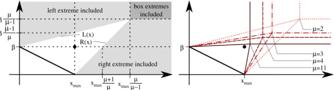
-distributions is to have a finite (resp. non-zero) derivative on the left extreme (resp. right extreme). The following theorem generalizes this result and shows that also for the weighted hypervolume indicator, the same necessary condition holds.Fig. 5. Influence of the choice of the reference pointr =(r1,r2)on optimal 2- (left) and optimal 10-distributions on the ZDT1 problem, in particular on the left extreme. Shown are the best approximations found within 100 CMA-ES runs forr=(1.01,1.01)(▽),r=(1.1,1.1)(◦),r=(2,2)(♦), and
r=(11,11)(△). Note that according to theory, the left extreme is never included in optimalµ-distributions and the lower bound onr1to ensure the right extreme isR1=3 [2].
Theorem 3.Let
µ
be a positive integer. Assume that f is continuous on[
xmin,
xmax]
, non-increasing, differentiable on]
xmin,
xmax[
and that f′is continuous on]
xmin
,
xmax[
and that the weight functionw
is continuous and positive. Iflimx→xminf′
(
x)
= −∞
, theleft extremal point of the front is never included in an optimal
µ
-distribution for IH,w. Likewise, if f′(
xmax
)
=
0, the right extremal point of the front is never included in an optimalµ
-distribution for IH,w.Proof. The idea behind the proof is to assume the extreme point to be contained in an optimal
µ
-distribution and to show a contradiction. In particular, the gain and loss in hypervolume if the extreme point is shifted can be computed analytically. A limit result for the case that limx→xminf′
(
x
)
= −∞
(andf′(
xmax)
=
0 respectively) shows that one can always increase the overall hypervolume indicator value if the outmost point is shifted; see alsoFig. 11. For the technical details, including a technical lemma, we refer toAppendix A.3on page96.Example 5. Consider the test problem ZDT1 [34] with a Pareto front described byf
(
x)
=
1−
√
xwithxmin=
0 andxmax=
1; seeFig. 9(a). The derivativef′(
x)
= −
1/(
2√
x)
equals−∞
at the left extremexminand the left extreme is therefore never included in an optimalµ
-distribution forIH,waccording toTheorem 3.Although one should keep the previous result in mind when using the hypervolume indicator, the fact that the extreme can never be obtained in the cases ofTheorem 3is less restrictive in practice. Due to the continuous search space for most of the test problems, no algorithm will obtain a specific solution exactly – and the extreme in particular – and if the number of points is high enough, a solution close to the extreme12will be found also by hypervolume-based algorithms. However, if the number of points is low the choice of the reference point is crucial and choosing it too close to the nadir point will massively change the optimal
µ
-distribution as can be seen exemplary for the ZDT1 problem inFig. 5.13Moreover, when using the weight function in the weighted hypervolume indicator to model preferences of the user towards certain regions of the objective search, one should pay attention to this fact by increasing the weight drastically close to such extremes if they are desired; see [1] for examples.4.1.2. Lower bound for choosing the reference point for obtaining the extremes
We have seen in the previous section that if the limit of the derivative of the front at the left extreme equals
−∞
(resp. if the derivative of the front at the right extreme equals zero) there is no choice of reference point that allows to have the extremes included in optimalµ
-distributions forIH,w. We assume now that the limit of the derivative of the front at the left extreme is finite (resp. the derivative of the front at the right extreme is not zero) and investigate conditions ensuring that there exists (finite) reference points ensuring to have the extremes in the optimalµ
-distributions.Lower bound for left extreme.
Theorem 4 (Lower Bound for Left Extreme). Let
µ
be an integer larger than or equal to 2. Assume that f is continuous on[
xmin,
xmax]
, non-increasing, differentiable on]
xmin,
xmax[
and that f′is continuous on]
xmin,
xmax[
andlimx→xmin−
f ′(
x
) <
∞
. If there exists aK2∈
Rsuch that for all x1∈ ]
xmin,
xmax]
K2 f(x1)w(
x1,
y)
dy>
−
f′(
x1)
xmax x1w(
x,
f(
x1))
dx,
(13)12 Although the distance of solutions to the extremes might be sufficiently small in practice also for the scenario ofTheorem 3, the theoretical result shows that for a finiteµ, we cannot expect that the solutions approach the extremes arbitrarily close.
13 The shown approximations of the optimalµ-distribution have been obtained by using the algorithm CMA-ES [20, version 3.40beta with standard settings] to solve the two-dimensional optimization problem ofRemark 2with the two leftmost points as variables and a boundary handling with penalties if the leftmost or rightmost point is outside[xmin,xmax](population size 20, best result over 100 runs shown).
then for all reference points r
=
(
r1,
r2)
such that r2≥
K2and r1>
xmax, the leftmost extremal point is contained in optimalµ
-distributions for IH,w. In other words, definingR2asR2
=
inf{
K2satisfying Eq.(13)}
,
(14) the leftmost extremal point is contained in optimalµ
-distributions if r2>
R2, and r1>
xmax.Proof. This proof is presented inAppendix A.4on page97.
Remark 4. The previous theorem states only an implicit condition forK2 and it is not always obvious whether a finite K2with the stated properties exists. There are different reasons for a non-existence of a finiteK2—although we assume that limx→xmin
−
f′
(
x
) <
∞
. One reason can be the fact thatf′(
x1)
is infinite for somex1∈ ]
xmin,
xmax]
such that the right-hand side of Eq. (13) is not finite and thereforeK2cannot be finite as well.Example 6, however, shows an example where f′(
x1
)
= −∞
for anx1∈ ]
xmin,
xmax]
andK2is still finite. Another possible reason for the non-existence of a finiteK2can be a choice ofw
such that the left-hand side of Eq. (13) is always smaller than the right-hand side—even assuming thatw
is continuous does not prevent such a choice ofw
.We will now apply the previous theorem to the unweighted hypervolume and prove anexplicitlower bound for setting the reference point so as to have the left extreme. This results recovers [2, Theorem 2].
Corollary 2 (Lower Bound for Left Extreme). Let
µ
be an integer larger than or equal to 2. Assume that f is continuous on[
xmin,
xmax]
, non-increasing, differentiable on]
xmin,
xmax[
and that f′ is continuous on[
xmin,
xmax[
. Let us assume that limx→xmin−
f′
(
x) <
∞
. IfR2
=
sup{
f′(
x)(
x−
xmax)
+
f(
x)
:
x∈ ]
xmin,
xmax]}
(15) is finite, then the leftmost extremal point is contained in optimalµ
-distributions for IHif the reference point r=
(
r1,
r2)
is such that r2is strictly larger thanR2and r1>
xmax.Proof. The proof is presented inAppendix A.5on page98.
Example 6. Consider again the DTLZ2 test function fromExample 1withf
(
x)
=
√
1
−
x2andf′(
x
)
= −
√
x1−x2 where
xmin
=
0 andxmax=
1. Assumew
=
1, i.e., the unweighted hypervolume indicatorIH. We see thatf′(
xmax)
= −∞
but nevertheless,R2is finite according to Eq. (15), namelyR2
=
sup
−
√
x 1−
x2(
x−
xmax)
+
1−
x2:
x∈ ]
x min,
xmax]
=
6√
3−
9≈
1.
18,
which can be obtained for example with a computer algebra system such as Maple.Lower bound for right extreme. We now turn to the case of the right extreme and address the same question as for the left extreme: assuming thatf′
(
xmax
)
̸=
0, can we find an explicit lower bound for the first coordinate of the reference point ensuring that the right extreme is included in optimalµ
-distributions? The following result holds.Theorem 5 (Lower Bound for Right Extreme). Let
µ
be an integer larger than or equal to 2. Assume that f is continuous on[
xmin,
xmax]
, non-increasing, differentiable on]
xmin,
xmax[
and that f′is continuous on]
xmin,
xmax[
and f′(
xmax)
̸=
0. If there exists aK1∈
Rsuch that for all xµ∈ [
xmin,
xmax[
−
f′(
xµ)
K1 xµw(
x,
f(
xµ))dx>
f(xmin) f(xµ)w(
xµ,y)
dy,
(16)then for all reference points r
=
(
r1,
r2)
such that r1≥
K1and r2>
f(
xmin)
, the rightmost extremal point is contained in optimalµ
-distributions. In other words, definingR1asR1
=
inf{
K1satisfying Eq. (
16)
}
,
(17) the rightmost extremal point is contained in optimalµ
-distributions if r1>
R1, and r2>
f(
xmin)
.Proof. This proof is presented inAppendix A.6on page98.
We will now apply the previous theorem to the unweighted hypervolume and prove an explicit lower bound for setting the reference point so as to have the right extreme. This results recovers [2, Theorem 2].
Corollary 3 (Lower Bound for Right Extreme). Let
µ
be an integer larger than or equal to 2. Assume that f is continuous on[
xmin,
xmax]
, non-increasing, differentiable on]
xmin,
xmax[
and that f′is continuous and strictly negative on]
xmin,
xmax]
. If R1=
sup
x+
f(
x)
−
f(
xmin)
f′(
x)
:
x∈ [
xmin,
xmax[
(18) is finite, then the rightmost extremal point is contained in optimalµ
-distributions for IHif the reference point r=
(
r1,
r2)
is such that r1>
R1and r2>
f(
xmin)
.Proof. The proof is presented inAppendix A.7on page99.
4.2. Number of points going to infinity
The lower bounds we have derived for the reference point such that the extremes are included are independent of
µ
. It can be seen in the proof that those bounds are not tight ifµ
is larger than 2. Deriving tight bounds is, however, difficult because it would require to know for a givenµ
where the second point of optimalµ
-distributions is located. It can be certainly achieved in the linear case (see [10]), but it might be impossible in more general cases. However, we want to investigate now howµ
influences the choice of the reference point so as to have the extremes. In this section, we will denoteRNadir1 andRNadir2 the first and second coordinates of the nadir point, namelyR1Nadir=
xmaxandRNadir2=
f(
xmin)
.We will prove that for any reference point dominated by the nadir point, there exists a
µ
0such that for allµ
larger thanµ
0, optimalµ
-distributions associated to this reference point include the extremes in case the extremes can be contained in optimalµ
-distributions, i.e., if−
f′(
xmin
) <
∞
andf′(
xmax) <
0. Before, we establish a lemma saying that if there exists a reference pointR1allowing t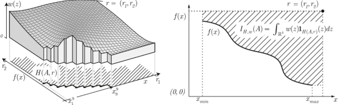
![Fig. 8. Lists for all ZDT, DTLZ, and WFG test problems and the unweighted hypervolume indicator I H : (i) the Pareto front as x ∈ [ x min , x max ] → f ( x ) , (ii) the density δ F ( x ) on the front according to Eq](https://thumb-us.123doks.com/thumbv2/123dok_us/895293.2615099/16.816.98.723.76.675/lists-problems-unweighted-hypervolume-indicator-pareto-density-according.webp)