Dissertation
DETECTOR DEVELOPMENT FOR DIRECTION-SENSITIVE DARK MATTER RESEARCH
by
HIDEFUMI TOMITA
B.S., University of California, San Diego, 2004
Submitted in partial fulfillment of the requirements for the degree of
Doctor of Philosophy 2011
First Reader
Steven P. Ahlen, Ph.D.
University Professor and Professor of Physics
Second Reader
Robert M. Carey, Ph.D. Associate Professor of Physics
I would love to thank my parents, Etsuo and Yoshiko, and my sister, Ai, for always be-lieving in and supporting me in my life journey. Although the life path I have chosen so far may be the furthest from what a typical Japanese man would pick, you were always there for me. I could not have accomplished such a big goal without your support. I would also love to thank Shelby Patton for loving and supporting me for the latter half of my graduate student career. Since I met you, I have become like a fish who found water. You taught me the joy of life and, thanks to you, I will always love my life with you.
I would like to thank Lora Brill for all the love and joy we shared together. I was so lucky to have spent part of my life with you - we grew together, we laughed together, and we cried together. I would not have been who I am without you. Also my best friend, Alvaro Roc-caro; it still hurts me when I think of having you lost so young. But, because of you, I can really appreciate what I have now, and I have enjoyed every single day of my life since then.
Thank you very much to my adviser, Professor Steve Ahlen, for guiding me through my graduate student career. I was very lucky to have joined your group at a most perfect tim-ing imaginable. You taught me disciplines and techniques that I will need as a scientist. Thank you very much to my friend/co-worker, Andrew Inglis, for helping me at work and being such a great friend. And I would love to thank all my friends - all international and American - for sharing an amazing time with me in my life.
DARK MATTER RESEARCH
(Order No. )
HIDEFUMI TOMITA
Boston University Graduate School of Arts and Sciences, 2011
Major Professor: Steven P. Ahlen, University Professor and Professor of Physics
ABSTRACT
The existence of Dark Matter was first proposed by Fritz Zwicky in 1933, based on the ob-served velocity distribution of galaxies in the Coma Cluster. Subsequent studies of visible mass and velocity distributions in other galaxies have confirmed Zwicky’s original observa-tion; there is now little doubt that Dark Matter exists. However, due to the fact that Dark Matter interacts very weakly through non-gravitational forces, nothing is known about the nature of Dark Matter. It is believed that Dark Matter particles are streaming toward the Earth, in the Earth’s rest frame, from the direction of the constellation Cygnus. Obser-vation of this so-called Dark Matter ’wind’ with a direction-sensitive dark matter particle detector would be compelling evidence that Dark Matter does consist of a gas of discrete particles as a new form of matter. The DMTPC collaboration is developing such a detector, and this thesis describes R&D work in support of that project. The DMTPC technique for looking for Dark Matter relies on Dark Matter particles interacting with atomic nuclei, causing the nuclei to recoil and to leave optical signals that can be detected. Since neu-trons are electrically neutral and collide with nuclei, they can mimic Dark Matter signals. Therefore, the reduction of neutron background is critical to the successful detection and identification of Dark Matter particles. One important aspect of this thesis is to fully understand and quantify neutron interactions with our detector. In addition to providing information for understanding Dark Matter experiments, this work also allows us to
number of neutron events in a variety of experimental runs both with and without neutron sources such as a neutron generator and252Cf. From these runs, we have obtained data for both elastic and inelastic interactions of neutrons of various energy ranges with detector gas nuclei. In this thesis, I will also discuss our current background data taking for the Dark Matter research and our plan for scaling up the detector to 100 m3 for a competitive Dark Matter search.
1 History and Theoretical Motivation of Dark Matter 1
1.1 Historical Background . . . 1
1.2 General Detection Method . . . 5
1.2.1 Detection Technique . . . 5
1.2.2 Daily/Seasonal Modulation . . . 6
1.2.3 Other Capabilities of the Detector . . . 9
2 DMTPC Detection Method 11 2.1 Fundamental Detector Concept . . . 11
2.2 CF4 Gas . . . 14
2.3 Neutron Detection . . . 20
3 DMTPC Detector 23 3.1 Detector Introduction . . . 23
3.2 First R&D Wire Chamber at MIT . . . 26
3.3 Prototype Dark Matter Detector at Boston University . . . 32
3.3.1 First Wire Chamber Components . . . 32
3.3.2 Improvement to Mesh Chamber . . . 40
3.3.3 EMCCD . . . 43
3.3.4 Up-To-Date DM Prototype Detector . . . 50
4 Fast-Neutron Tests with Prototype DM Detector at MIT 53
4.1.1 Introduction to Cf Neutron Runs . . . 53
4.1.2 252Cf Run Data with Pure CF4 Gas in BU Prototype . . . 55
4.1.3 Electron Diffusion Check in 40 torr CF4 Gas . . . 59
4.1.4 252Cf Run Data with Gas Mixture of CF4 and4He in BU Prototype 61 4.1.5 Electron Diffusion Check in Gas Mixture of 40 torr CF4 and 4He . . 62
4.1.6 Directionality Capability of our Detector . . . 62
4.2 Fast Neutron Detection from D+T Neutron Generator at MIT . . . 69
4.2.1 Introduction to D+T Neutron Generator Neutron Runs . . . 69
4.2.2 D+T Neutron Generator Run Data with Pure CF4 Gas in BU Pro-totype . . . 71
5 Preliminary TPC Experiment with Xe Gas 79 5.1 Scintillation Characteristics of Xe Gas . . . 79
5.2 Non-Linearity of the Stopping Power of Xe Gas . . . 83
6 Preparations for the Background Neutron Detection Experiment 87 6.1 EMCCD and PMT Dual Readout System . . . 87
6.2 Two Experiments for the BU Prototype Chamber Quantification . . . 90
6.2.1 Spark Experiment . . . 90
6.2.2 Correlation Experiment . . . 95
6.2.3 Electron Diffusion Effect on EMCCD Readout . . . 100
7 Thermal Neutron Measurement with BU Prototype Chamber 103 7.1 Thermal Neutron Absorption of 3He . . . 103
7.2 Thermal Neutron Data Measurement . . . 106
7.3 Thermal Neutron Data Result . . . 110
7.4 Determining the 3D Full Track Length . . . 114
7.5 Change of Gas Gain and Energy Threshold . . . 115 vii
8 Cylon: A New Direction-Sensitive Fast Neutron Detector 127
8.1 Introduction to Cylon . . . 127
8.2 Thermal Neutron Capture Event Data with Cylon Detector . . . 140
8.2.1 Electron Drift Velocity . . . 140
8.2.2 Gain Variation Problem . . . 142
8.2.3 Applying Data Correction to Improve the Gain Non-Uniformity . . . 146
8.2.4 Change of Triggering System . . . 146
8.2.5 Thermal Neutron Flux by Cylon . . . 149
8.3 Cosmic Ray Neutron Data with Cylon as a Fast Neutron Detector . . . 151
8.3.1 Initial Motivation of Cylon Fast Neutron Detector . . . 151
8.3.2 Background Cosmic Ray Neutron Data by Cylon . . . 156
8.4 Detector Improvements . . . 159
8.4.1 Improvement for Active Interrogation . . . 159
8.4.2 Improvement for Gas Gain . . . 161
9 Dark Matter Background Data Run by Cylon 163 9.1 20-Day Background Data by Cylon with Gas Mixture of 3He . . . 163
9.2 Particle Identification in Large Energy or Long Track Region . . . 166
9.3 Particle Identification at MeV Region . . . 167
9.4 Particle Identification at Dark Matter Energy Region . . . 170
9.5 Cosmic Ray Neutron Induced Inelastic Recoils and Summary . . . 172
10 Conclusion and Next Goal 177 10.1 Current Status of DMTPC Collaboration . . . 177
10.2 1 m3 Dark Matter Detector . . . 178
10.2.1 Sensitivity and Limits . . . 178
10.2.2 Design . . . 180 viii
Bibliography 184
Curriculum Vitae 190
1.1 Dark Matter evidence . . . 2
1.2 WMAP data . . . 3
1.3 Bullet cluster . . . 4
1.4 SD and SI exclusion limits . . . 6
1.5 Anual modulation . . . 7 1.6 DAMA/LIBRA data . . . 8 1.7 Daily modulation . . . 9 2.1 DMTPC detection method . . . 12 2.2 CF4 scintillation spectrum . . . 14 2.3 CF4 electron-to-photon ratio . . . 15
2.4 Energy loss of a traveling charged particle . . . 18
2.5 Electron mobility of CF4 gas . . . 19
2.6 Electron diffusion experiment setup . . . 20
2.7 Electron diffusion experiment result . . . 21
2.8 High-energy neutron cross section . . . 22
2.9 Thermal neutron cross section . . . 22
3.1 . . . 25
3.2 Data acquisition schematics . . . 26
3.3 First generation R&D chamber . . . 27
3.4 QE of Kodak KAF-0401 . . . 28 x
3.6 First successful image capture of anα particle . . . 30
3.7 BU prototype chamber . . . 34
3.8 BU prototype wire frames . . . 35
3.9 Wire transfer frame from BNL . . . 35
3.10 BU prototype wire chamber setup . . . 36
3.11 QE of Kodak KAF-1603ME . . . 37
3.12 First generation BU prototype dual-readout system . . . 38
3.13 First correlated data of anα particle by CCD and PMT . . . 39
3.14 BU prototype electron field cage . . . 41
3.15 BU prototype mesh amplification plane . . . 42
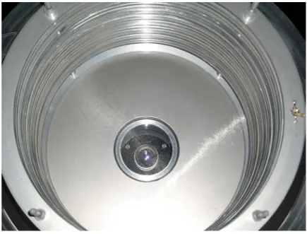
3.16 BU prototype cathode mesh and lens . . . 43
3.17 QE of Kodak KAF-1001E . . . 44
3.18 EMCCD signal-to-noise ratio . . . 45
3.19 QE of EMCCD . . . 46
3.20 EMCCD chip pixels schematics . . . 47
3.21 EMCCD-LED setup . . . 49
3.22 PMT-LED setup . . . 49
3.23 Photon-to-ADU conversion result . . . 49
3.24 Schneider Xenon 0.95/17 lens . . . 50
3.25 Upgraded BU prototype chamber . . . 51
3.26 Glass window light transmission . . . 52
4.1 252Cf . . . 54
4.2 252Cf run in a pure 40 torr CF 4 . . . 56
4.3 SRIM simulation of 252Cf run in a pure 40 torr CF4 . . . 56
4.4 Close-up of252Cf-induced nuclear recoil track in a pure 40 torr CF4 . . . . 58
4.5 252Cf-induced nuclear recoil tracks in a pure 40 torr CF4 . . . 59 xi
4.7 Diffusion result in 40 torr CF4 gas . . . 61
4.8 252Cf run in a gas mixture of 40 torr CF4 and 600 torr 4He . . . 63
4.9 SRIM simulation of 252Cf run in a gas mixture of 40 torr CF4 and 600 torr 4He . . . . 63
4.10 Close-up of 252Cf-induced nuclear recoils in a gas mixture of 40 torr CF4 and 600 torr 4He . . . 64
4.11 252Cf-induced nuclear recoil tracks in a gas mixture of 40 torr CF4 and 600 torr 4He . . . . 65
4.12 Diffusion result in a gas mixture of 40 torr CF4 and 600 torr 4He . . . 66
4.13 MIT NW-13 laboratory schematics . . . 67
4.14 Angular distribution of nuclear recoils in a gax mixture of 40 torr CF4 and 600 torr 4He . . . 68
4.15 Angular distribution of nuclear recoils in a pure 40 torr CF4 gas . . . 70
4.16 D+T neutron generator . . . 70
4.17 Neutron cross sections for both elastic and inelastic interactions . . . 72
4.18 Close-up of high-energy-neutron-induced nuclear recoils in a pure 40 torr CF4 gas . . . 73
4.19 High-energy-neutron-induced elastic nuclear recoil tracks in a pure 40 torr CF4 gas . . . 74
4.20 High-energy-neutron-induced inelastic nuclear recoil tracks in a pure 40 torr CF4 gas . . . 74
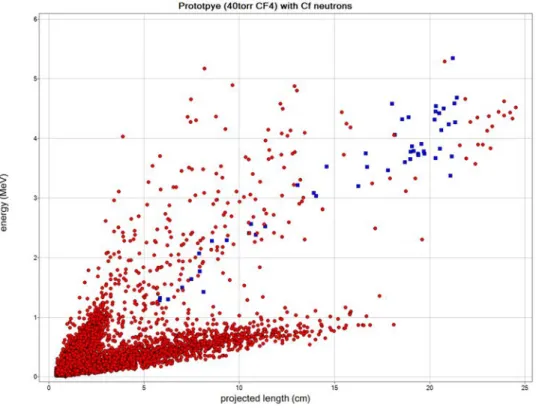
4.21 Range-vs.-energy scatter plots comparison from252Cf and neutron generator runs . . . 75
4.22 Table of inelastic neutron interaction result . . . 76
4.23 Inelastic neutron interaction data comparison to expected values . . . 77
4.24 High-energy-neutron-induced 3α production candidates . . . 78
5.2 α particle track comparison in CF4 and Xe gases . . . 81
5.3 α particle track in Xe gas with varying CF4 gas pressure added . . . 82
5.4 α particle track in Xe gas with varying anode voltages . . . 84
5.5 Non-linearity test of an α particle track in Xe gas mixture . . . 84
5.6 Non-linearity test result . . . 85
6.1 New dual-readout system of EMCCD and PMT . . . 88
6.2 Spark test setup . . . 91
6.3 α particle range in a pure 40 torr CF4 gas . . . 92
6.4 Table of spark test result . . . 93
6.5 Electron drift velocity test setup . . . 96
6.6 Horizontally-moving α particles . . . 96
6.7 α particles traveling at 45◦ angle . . . 97
6.8 α particles traveling at 60◦ angle . . . 97
6.9 Electron drift velocity test result . . . 99
6.10 Electron diffusion effect on EMCCD data measurements . . . 102
6.11 Electron diffusion effect on PMT data measurements . . . 102
7.1 Expected range of P+T tracks in a gas mixture of 40 torr CF4 and 100 torr 3He . . . 104
7.2 Sample image of P+T tracks in a gas mixture of 40 torr CF4 and 100 torr3He105 7.3 P+T track examples . . . 107
7.4 ’bent’ P+T track examples . . . 108
7.5 Background α track examples . . . 109
7.6 Range vs. energy scatter plot by EMCCD . . . 111
7.7 Range vs. energy scatter plot by PMT . . . 112
7.8 Linearity of EMCCD and PMT data . . . 113
7.9 Electron drift velocity in a gas mixture of 40 torr CF4 and 100 torr 3He . . 115 xiii
7.11 ’40 torr CF4 + 100 torr He’ run scatter plot after drift velocity correction 117 7.12 Close-up of ’40 torr CF4 + 100 torr3He’ run scatter plot after drift velocity
correction . . . 118
7.13 ’40 torr CF4+ 100 torr3He’ run scatter plot, with SRIM data superimposed, after drift velocity correction . . . 119
7.14 Change of gain over time . . . 120
7.15 Change of energy threshold over time . . . 122
7.16 Polar angular distribution of data . . . 124
7.17 Change of thermal neutron event rate over time . . . 125
8.1 Cylon . . . 128
8.2 Cylon lens . . . 130
8.3 Cylon lens drop-off at edges . . . 131
8.4 Cylon PMT . . . 132
8.5 Cylon electron amplification region . . . 133
8.6 Cylon resolution byα particles . . . 135
8.7 Linearity of Cylon EMCCD + PMT . . . 136
8.8 Cylon electron field cage . . . 138
8.9 Cylon electron diffusion result . . . 139
8.10 Projected- vs. vertical-track-length in Cylon . . . 141
8.11 Electron drift velocity in Cylon . . . 142
8.12 Cylon3He run data scatter plot . . . 143
8.13 Cylon electron gain fluctuation . . . 144
8.14 Cylon3He run data scatter plot - gain variation corrected . . . 147
8.15 Backgroundα track examples in Cylon . . . 149
8.16 Polar angular distribution of data in Cylon . . . 150
8.17 Change of energy threshold over time in Cylon . . . 151 xiv
8.19 Comparison of thermal neutron event rates by prototype chamber vs. Cylon 153
8.20 Cosmic-ray-neutron-induced track examples in Cylon . . . 155
8.21 Azimuthal distribution of particle tracks in Cylon . . . 156
8.22 Change of Cosmic-ray neutron event rate over time in Cylon . . . 157
8.23 Cylon background run scatter plot, with SRIM data superimposed, after drift velocity correction . . . 158
8.24 Pulsing capability of Cylon detector for an active interrogation . . . 160
8.25 Gas Filtration . . . 162
9.1 Dark Matter Background Data Run with Cylon . . . 164
9.2 Dark Matter Background Data Run with Cylon with SRIM simulation . . . 165
9.3 Cylon DM run: α Background . . . 166
9.4 Cylon DM run: Proton and Muon Background . . . 167
9.5 Cylon DM run: High Energy C or F Recoils . . . 168
9.6 Cylon DM run: MeV Energy Region . . . 169
9.7 Cylon DM run: Two Bands of Partially-Contained P+T Tracks . . . 169
9.8 Cylon DM run: 4He Recoils . . . 170
9.9 Cylon DM run: Low Energy Dark Matter Region . . . 171
9.10 Low Energy C or F Nuclear Recoils . . . 172
9.11 20-day Dark Matter Background Run Total Sensitive Volume . . . 173
9.12 Cylon DM run: Inelastic Collision Event 1 . . . 174
9.13 Cylon DM run: Inelastic Collision Event 2 . . . 174
9.14 Cylon Measurement Comparison to Other/Calculations . . . 175
9.15 Cylon Measurement Cosmic Ray Proton at Sea Level . . . 176
10.1 WIPP . . . 178
10.2 DMTPC exclusion limit in MSSM model . . . 179
10.3 DMTPC 1 m3 Detector Conceptual Design . . . 181 xv
3He Helium-3
4He Helium-4
ADU Analog-to-Digital Unit
AMS Alpha Magnetic Spectrometer
BNL Brookhaven National Lab
BU Boston University
CCD Charge-Coupled Device
CDM Cold Dark Matter
CF4 Carbon Tetrafluoride or Tetrafluoro Methane
DM Dark Matter
DMTPC Dark Matter Time Projection Chamber
EMCCD Electron Multiplying Charge-Coupled Device
eV Electron Volt
GEM Gas Electron Multiplier
GeV Giga Electron Volt
keV Kilo Electron Volt
LHC Large Hadron Collider
LSP Lightest Supersymmetric Particle
MeV Mega Electron Volt
M.F.P. Mean Free Path
MicroMEGAS MicroMEsh GAseous Structure
m.w.e. Meters Water Equivalent
PMT Photo Multiplier Tube
PRB Physics Research Building
QE Quantum Efficiency
Rn Radon
SRIM the Stopping and Range of Ions in Matter
Th Thorium
TPC Time Projection Chamber
U Uranium
WIMP Weakly Interacting Massive Particle
WMAP Wilkinson Microwave Anisotropy Probe
Xe Xenon
History and Theoretical Motivation of
Dark Matter
1.1
Historical Background
In the 1930s during his observation of the Coma Cluster of galaxies, Fritz Zwicky discov-ered that the velocities of those galaxies were much greater than what the visible matter alone should have caused (Zwicky, 1933, 1937). In fact, without some unseen mass within the cluster, the observed velocities were so great that the galaxies would have escaped the cluster. Based on the quantity of light emanating from those galaxies, Zwicky concluded that the total mass required to produce the velocity distribution was an order of magnitude greater than what he had observed. This result led him to propose the existence of some sort of invisible and unknown matter in the Universe, which he named ”dunkle (kalte) Materie”.
In the 1970s, a group of scientists led by Vera Rubin studied the rotational velocities of individual spiral galaxies and concluded, with unambiguous evidence, that the theory pro-posed by Zwicky was correct (Rubin et al., 1978). The center of each spiral galaxy has the highest concentration of visible matter, such as stars, etc. Thus, the greatest amount of light is observed from this region. As the distance from the center increases, the amount of light observed decreases. This led astronomers to assume that most of the mass was
(a) (b)
Figure 1.1: (a) Rotational velocities as a function of the distance from the center of each galaxy. (b) Internal mass contained within a disk of radius r, as a function of r, which is the distance from the center of the galaxy (Rubin et al., 1978).
concentrated at the center of the rotating galaxies. On such a large scale, gravitational in-teraction dominates the motion of the galaxies/stars, and it was natural to believe that the velocities of visible matter would decrease as the distance from the center of each galaxy increased. However, what Rubin discovered was the complete opposite of this presumption; the rotational velocities of visible matter stayed constant from the center to the perimeter of the galaxies (see Fig. 1.1(a)), despite the fact that there was not nearly enough visible mass observed to account for the visible matter’s velocity. Rubin then proposed that most of the visible matter was bundled within a huge spherical halo of dark matter, which provides the necessary mass for the visible matter to rotate with the observed velocities (see Fig. 1.1(b)).
In 2001, NASA launched the Wilkinson Microwave Anisotropy Probe (WMAP) to make precision measurements of the Cosmic Microwave Background radiation (see Fig. 1.2). The measurements revealed that only 4.6 % of the entire energy of the Universe is made of or-dinary or baryonic matter, which constitutes standard model particles such as protons, neutrons, or electrons. It also concluded that 72.1 % of the energy in the Universe is made
Figure 1.2: Seven year WMAP data showing the temperature fluctuations that occurred 13.7 billion years ago (The WMAP Science Team).
up of Dark Energy, which is believed to be responsible for the acceleration of the Universe’s expansion. The remaining 23.3 % of energy is believed to be made up of Dark Matter, the subject of this thesis (Komatsu et al., 2010; Bennett et al., 2003).
More evidence for the existence of Dark Matter came from weak gravitational lensing ob-servations of two colliding clusters of galaxies, called the ’bullet cluster.’ In their paper, Clowe et al. presented the analysis of the details of the two colliding galaxies (Clowe et al., 2006). The two galaxies collided with a velocity of 4500 km/s. After the collision, there is a clear separation between the concentrations of visible matter and the invisible matter. The green lines in Fig. 1.3 show the gravitational contour based on weak lensing measurements and the distribution of Dark Matter is depicted in blue. During the merging event of the two clusters, ordinary gas experienced ram pressure, and the motion of the visible part of the galaxies slowed. This is shown in the color plots of Fig. 1.3. However, Dark Matter does not experience such a force, resulting in the clear separation of the two species of particles baryonic and non-baryonic matter. This phenomenon presented strong evidence for the existence of Dark Matter. There is no question that the majority of the matter in the Universe consists of non-baryonic cold Dark Matter (Bertone et al., 2005). Dark
(a) (b)
Figure 1.3: (a) The merging cluster 1E0657-558. (b) Image from NASA’s Chandra X-ray Observatory (Clowe et al., 2006).
Matter is some type of matter that is heavy enough to cause the orbital velocity of galaxies to be constant, regardless of the distance from galaxies’ centers and the amount of visible matter within the galaxies.
If Dark Matter does exist, it is very likely that it would follow new physics laws beyond the Standard Model of particle physics. One of the leading candidates of Dark Matter is called Weakly Interacting Massive Particles (WIMPs) (Jungman et al., 1996). WIMPs are stable, carry zero electric charge, and interact weakly with baryonic matter. One of the theories that attempts to explain Dark Matter beyond the Standard Model of physics is the theory of Supersymmetry. According to this theory, the lightest supersymmetric par-ticle (LSP) is the Dark Matter parpar-ticle and would interact with ordinary matter through extremely small interaction cross sections. In this model, the conserved quantum number (called R-parity) prevents such LSP particles from decaying into ordinary baryonic matter. They are therefore considered to be stable over the life of the Universe.
1.2
General Detection Method
1.2.1 Detection TechniqueThere are three ways to look for Dark Matter. One is with a particle collider such as the LHC (Kane and Watson, 2008), which is expected to make new discoveries in particle physics. Another detection method is ’indirect detection.’ Such experimental methods include the Alpha Magnetic Spectrometer (AMS) project (Alcaraz et al., 1999). In an indirect detection method, the detectors are launched into outer space and look for WIMP annihilation products. The big challenge in such an experiment is the separation of the Dark Matter signal from the large background that originates in astronomical events such as supernovae. Finally, the method we utilize is called ’direct detection’ of Dark Matter (Gaitskell, 2004). This detection method relies on Dark Matter’s interaction with target nuclei through its extremely weak interaction rate. We attempt to detect the scattering of the target nucleus and energy deposited as it recoils from a collision event with an incoming Dark Matter particle.
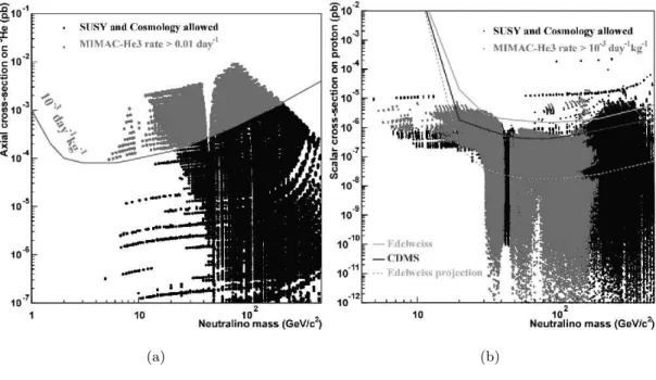
The expected mass of Dark Matter candidates varies from a few GeV to hundreds of GeV(Bertone et al., 2005). In our experiment, we use a time projection chamber (TPC) filled with low pressure carbon tetrafluoride (CF4) gas. Typical WIMP-induced nuclear recoils in such a detector are expected to deposit energy of a few to 100 keV. Dark Matter interactions with ordinary matter would occur through either axial (spin-dependent) or scalar (spin-independent) interactions (see Fig. 1.4). Through the spin-dependent interac-tion with Dark Matter, a fluorine atom is considered to be the most sensitive candidate (Ahlen, 2010). The next most sensitive target would be Xe, followed by iodine and ger-manium. It has been shown that an LSP Dark Matter candidate may have a fairly large cross section through the spin-dependent interaction (Moulin et al., 2005; Gainer, 2010). As I will discuss later in Sec. 2.2, CF4 gas is known for its good scintillation efficiency, low transverse electron diffusion effect and is non-flammable and non-toxic; thus, using fluorine
(a) (b)
Figure 1.4: Expected cross sections calculated in non-MSSM model of (a) spin-dependent and (b) spin-independent interactions on nucleon (Moulin et al., 2005).
as the target gas for the direct detection is a great advantage.
1.2.2 Daily/Seasonal Modulation
In our direct detection method, we attempt not only to identify the energy deposited by Dark Matter induced nuclear recoils, but also the direction of those recoil particles. In a simple Dark Matter halo model, our Solar System rotates around the center of the Milky Way Galaxy with a velocity of approximately 220 km/s within a spherical halo of Dark Matter. In this orbital motion, the direction of the Solar System is pointing towards the constellation Cygnus. Under the simple non-dissipative Dark Matter halo model, the Dark Matter particles are expected to be distributed by the Maxwell-Boltzmann distribution (Navarro et al., 1996; Ullio and Kamionkowski, 2001). From our reference frame on Earth, it seems as if our Solar System is moving through a sea of Dark Matter, due to the rota-tional motion of the Solar System around the center of the Milky Way Galaxy. Thus, the
Figure 1.5: Illustration of an annual modulation. The Earth rotates around the Sun with the rotational inclination of roughly 60 degrees relative to the motion of the Solar System itself rotating around the center of the Milky Way Galaxy.
direction of the Dark Matter flying towards us seems to originate from the direction of the constellation Cygnus. This is called Dark Matter wind. Because the Earth spins on its axis of rotation, the direction of Dark Matter wind changes continuously. This is called a daily modulation. In our experiment, we put emphasis on the directionality characteristics of Dark Matter wind due to the daily modulation effect.
The Earth rotates around the Sun with an inclination of roughly 60 degrees relative to the plane of rotational motion of the Solar System around the center of the Milky Way Galaxy. When the vector of the Earth’s motion lines up with that of the Solar System, the net Earth rotational velocity with respect to the rest of the Milky Way Galaxy reaches its maximum. This occurs during summer time in the northern hemisphere (see Fig. 1.5). Conversely, the total velocity reaches its minimum during the winter, so the amplitude of the Earth’s total velocity relative to the galactic rest frame fluctuates up to a few percent throughout the entire year. This is called an annual modulation. If Cold Dark Matter
Figure 1.6: The annual modulation measurement of Dark Matter signals from DAMA/LIBRA (Bernabei et al., 2008).
is indeed distributed in the way mentioned above, the velocity of the Dark Matter par-ticles flying towards us from the direction of the constellation Cygnus would fluctuate accordingly. Thus, the energy spectrum of Dark Matter induced nuclear recoils for the elastic scattering events would also fluctuate due to the annual modulation (Drukier et al., 1986; Freese et al., 1988). DAMA/LIBRA claims that they measured this Dark Matter induced annual modulation signal in their experiment (Bernabei et al., 2008). Their mea-surement shows the annual modulation of the signal amplitude (see Fig. 1.6). However, their claim has not been broadly accepted. Because background particles such as neutrons would strongly mimic the elastic scatter of Dark Matter particles of target nuclei, their measurements are too ambiguous to argue convincingly that they have only recorded the Dark Matter signals. DAMA’s result has also been excluded by other experiments such as XENON100 or CDMS (Aprile et al., 2010).
In order to make a clean identification of Dark Matter particle collision events, one needs to employ a technique that neatly separates the actual Dark Matter signals from back-ground noise. The technique we use is called a daily modulation (see Fig. 1.7). Due to the daily motion of the Earth, a detector on the Earth’s surface would observe the direc-tion of the incident Dark Matter wind to shift accordingly. For example, for a detector
Figure 1.7: Illustration of a daily modulation. Due to the change of the detector position over 12 hours, the direction of the Dark Matter wind shifts accordingly (Sciolla, 2009). placed in Boston, the Dark Matter wind direction changes by roughly 96 degrees over 12 hours. Thus, if one had the capability of detecting the direction of the Dark Matter wind, the direction of the resultant signal would shift by the same amount. Showing this result together with the energy spectrum due to the Dark Matter velocity would provide unambiguous evidence for the existence of Dark Matter. Although it is very important to identify background particles such as neutrons, only Dark Matter particles would produce such a shift of the incident direction presented by the daily modulation. The anticipated Dark Matter signal with directionality by the daily modulation is much more obvious than the data relying only on the seasonal modulation. Mere event rate comparison of forward and backward direction oriented Dark Matter signals gives roughly an order of magnitude difference (Spergel, 1988).
1.2.3 Other Capabilities of the Detector
So far I have only mentioned the direct detection of an elastic collision of Dark Matter off the target nuclei. Recently, however, the possibility of Dark Matter inelastic collisions have also been pointed out (Cui et al., 2009; Chang et al., 2009). The basic assumption in this theory is that the Dark Matter particles would have both ground and excited states that
are separated by roughly 100 keV. When the coherent inelastic scatter occurs, the Dark Matter particle gets shifted into its higher energy state. Because of the inelastic collision, a new particle, heavier than Dark Matter, will be formed and continue moving in the incident direction of the Dark Matter particle. In their model of Dark Matter, with a Dark Matter particle mass of 250 GeV, Chang et al. estimated an expected count rate of 0.5 /kg/day. Essentially any experiment with a direct detection method could be integrated into this technique. In our experiment, the use of Xe gas would be ideal for this method because the expected Dark Matter mass is rather close to that of the target Xe atoms. Furthermore, no changes would have to be made to our detector in order to search for inelastic collisions; we would simply switch the target gas from CF4 to Xe. Because Xe is very heavy, it would not be too difficult to reach a high target mass with our TPC detector. Although very preliminary, I will show the first study of our prototype Dark Matter detector with Xe gas later in this dissertation (see Chap. 5).
As mentioned earlier, among all the backgrounds in Dark Matter detection, neutron-induced nuclear recoils are the worst because they mimic those from Dark Matter. In Dark Matter experiments, it is very important to shield the detector actively and/or pas-sively from the neutron background. One effective method to achieve this goal is to place the detector deep in a mine so that one can minimize the effect of the cosmic ray back-ground. In this dissertation, I will discuss and quantify our detector’s background neutron measurements capability, which is necessary for the DMTPC Dark Matter experiment.
DMTPC Detection Method
2.1
Fundamental Detector Concept
The DMTPC (Dark Matter Time Projection Chamber) collaboration involves physicists from Boston University, Brandeis University and Massachusetts Institute of Technology. The basic idea of the DMTPC detector concept is shown in Fig. 2.1. The main components of the detector are the anode plate, grid mesh, cathode mesh and field cage rings. Positive high voltage is applied onto the anode, whereas the grid mesh is held at ground (potential); thus, a very intense electric field is created between the two. Inside the detector is filled with low pressure CF4 gas.
When a Dark Matter particle collides with a fluorine nucleus in the detector, it transfers some energy and momentum to the fluorine recoil with typical energies on the order of a few tens of keV. In the inelastic Dark Matter model, the target gas would be Xe. For a neu-tron detector, it works exactly the same except that most of the elastic scattering events occur off target helium atoms of an added 4He gas because of 4He’s large cross section with neutrons. In a low pressure TPC at 40 torr CF4 gas, a Dark Matter-induced fluorine recoil results in a length on the order of a couple of millimeters. When an incident Dark Matter particle collides with a fluorine nucleus, the nucleus is liberated and recoils with some kinetic energy, accompanied by one or more electrons. When this positive ion travels
through the gas, it loses energy by ionizing other atoms and molecules along its path. CF4 has a W value of 54 eV, so the traveling ion loses kinetic energy by an average of 54 eV at each ionization event along the path. The cathode mesh is kept at negative high voltage so that the ionization electrons will travel towards the grounded grid mesh and into the ampli-fication region. When they reach the ampliampli-fication region, which has a much more intense electric field than the drift region, those ionization electrons multiply (electron cascade) with a typical gain of 104 to 105. These so-called ’avalanche’ electrons excite ions of CF4 and cause scintillation of red light to occur (Pansky et al., 1995; Fraga et al., 2003). The photons emitted from this event travel towards the charge-coupled device camera (CCD camera) and photo multiplier tube (PMT) and will be captured as a light signal by those devices. The lens attached to the CCD camera is set to focus on the amplification region so that the 2D particle track projection onto the amplification region will be captured as data by the CCD camera. Although it depends on what type of particle is being measured, a typical charged particle in our experiment with an energy less than the order of MeV will travel only on the order of nanoseconds or less before it comes to rest. This is short compared to the drift time of the electrons as they move toward the anode. When the first light signal above the threshold from either head or tail of the moving particle hits the PMT, it triggers both the CCD and PMT to start recording the information. The camera’s minimum exposure time achievable is at least a factor of 100 greater than the actual time of particle motion; thus, there is no ambiguity about whether the particle is fully or only partially contained within the CCD image as long as the track occurred within the cam-era’s view. Because the PMT is a fast device, it has no problem obtaining an unambiguous signal from the drifting electrons in the detector. Depending on the vertical component of the travelling particle, PMT signals can come in various shapes over time, but they will measure the time between the arrival of the first and last electron at the amplification stage.
(a) (b)
Figure 2.2: (a) Pure CF4 spectrum measured by A. Kaboth of DMTPC collaboration (Kaboth et al., 2008). (b) Spectrum of gas mixture4He + 40 % CF4 (Fraga et al., 2003).
2.2
CF
4Gas
For our Dark Matter TPC experiment with optical readout, CF4 is an ideal gas for multiple reasons. First, fluorine is one of the most sensitive particles to spin-dependent interactions with a Dark Matter particle. It is crucial, however, to use this detector gas at a low pressure so that the fluorine tracks will be long enough to measure. CF4 gas is non-flammable and non-toxic, and it is known for its good scintillation efficiency in the red region, and for its low transverse diffusion of the drifting electrons (Christophorou et al., 1996). Fig. 2.2 illus-trates the spectrum of pure CF4 gas and its mixture with4He gas. What we can learn from them is that the CF4 gas dominates in the scintillation characteristics at the red optical region. Many CCD cameras have their highest quantum efficiency at the red region; thus, the use of CF4gas is very advantageous in our optical-readout technique. The DMTPC has measured the photon per electron ratio in the electron avalanches in a pure CF4 gas, us-ing a sus-ingle wire proportional chamber. As Fig. 2.3 shows, the ratio is approximately 34 %.
Figure 2.3: A linear fit to the number of photons vs. number of electrons from the electron avalanche in the detector’s electron amplification region (Kaboth et al., 2008).
The number of photons acquired from a single fluorine recoil may be approximated in the following equation. For this estimation, I assume all the parameters as explained below.
γ =Krecoil×12 ×WCF1
4
×Ge×Effe→γ×4Sπ Dlens2×Tlens×Twindow×QE×Tgrid×Tcathode
Krecoil (recoil fluorine energy) = 30 keV
WCF4 (average energy to produce electron-ion pair in CF4 gas = 54 keV
Ge (gas electron gain) = 105
Effe→γ (scintillation efficiency) = 0.34
Slens (lens surface area - assume use of Canon 85 mm f/1.2 lens) = 47
D (lens-to-anode distance in cm) = 35
Tlens (lens transmittance in the red region) = 0.85
Twindow (glass window transmittance in the red region) = 0.9
QE (quantum efficiency of the Apogee U6 camera) = 0.65 Tgrid (grid mesh spatial transmission) = 0.8
In this simple model, it is suggested that we would acquire 9,200 photons from a 30 keV fluorine recoil induced by the collision with a Dark Matter particle. The combination of the Canon 85 mm lens and Apogee Alta U6 camera is being used as a part of our DMTPC detector in the WIPP (Waste Isolation Pilot Plant) mine in Carlsbad, New Mexico for the initial background study. In a typical setup, each CCD pixel maps about 300 µm by 300 µm of real space, and a 30 keV recoil would be distributed over about 10 pixels, so each pixel will contain an average of 920 photoelectrons. The Alta U6 camera has a typical RMS readout noise of 8 electrons; thus, the typical signal-to-noise ratio of such a detector would be as large as 115.
In our standard data taking, we employ a pressure of 40 torr for the CF4 gas in the detec-tor. This is a low enough pressure that typical Dark Matter-induced fluorine recoils with energies of the order of tens of keV will travel for a couple of millimeters. This enables us to observe the recoil track with directionality. An even lower pressure would work better in terms of the ratio of particle track length vs. track width after some transverse elec-tron diffusion; however, when the pressure of CF4 gas becomes too low, we begin to face discharge problems in our high voltage amplification system before reaching enough gain in this region. Unfortunately, not much is known about the electric discharge mechanism, especially with the specific gas mixture and pressure settings we are interested in using with CF4 gas. After some trial-and-error, we have come to the conclusion that 40 torr of CF4 gas pressure is the optimum combination and has become our standard data-taking mode for the TPC chamber. It is also hard to get large detector mass with very low pressure.
Our detector relies on the scintillation light that occurs from the drift and cascade electrons exciting the CF4 gas molecule ions. When a charged recoil particle travels through such a gas detector, it continuously loses its energy along its path by ionizing the gas atoms and molecules. However, it does so at different rates along its trajectory (see Fig. 2.4). When
the energy of the recoil particle is greater than the so-called ’Bragg peak’ energy, its rate of energy loss increases as it loses energy. When it reaches the Bragg peak energy, where the particle is losing the greatest amount of energy per unit distance travelled, the ionization, as well as subsequent light collected, is at its greatest value. If the particle starts with energy less than the Bragg peak energy, the energy loss per unit distance travelled, and light collected along the path, will decrease along the path. With the knowledge of this light distribution along the path length for either situation, we can identify the direction of moving particles, which we call a ”head-tail” effect (Dujmic et al., 2008).
After the ionization event in the TPC, the ionization electrons start traveling against the direction of the drift electric field created in the field cage. During this drifting motion, each electron makes copious numbers of collisions with the electrons of the gas molecules. This causes the trajectory of each electron to be not straight; thus, the electrons are mov-ing towards the amplification region takmov-ing random paths. In effect, when the stream of electrons from the initial particle ionization track reach the amplification region for the scintillation, the measured transverse width of the particle track becomes much wider than what it really is. This is called electron diffusion, and it is related in a non-linear fashion with how far the electrons have drifted, what the pressure of the gas is, and the strength of the drift electric field (Christophorou et al., 1996; Ahlen, 2010). The amount of electron diffusion can be described in the following equation.
σdif f usion= q Z N · q 2 µD e N E
Z: electron drift distance N: number density of molecules
D: transverse electron diffusion constant
µe: electron mobility
Figure 2.4: An α particle travelling from left to right through the gas mixture of 40 torr CF4 and 600 torr 4He. The black histogram represents the actual data from the above CCD image, which shows the great agreement with the SRIM Monte Carlo simulation (The Stopping and Range of Ions in Matter) of the stopping power (red markers). Three locations where the particle track is being cut are due to the 530µm fishing wires as spacers between the anode and grid. The energy of theα particle is about 4.8 MeV, and at such a low energy, the stopping power can be approximated by the Bethe-Bloch formula presented in the above plot.
Figure 2.5: The rate of electron diffusion coefficient over the electron mobility as a function of the drift electric field applied over the number density of CF4 gas (Christophorou et al., 1996).
Fig. 2.5 shows the relationship between the amount of electron diffusion coefficient and the drift electric field applied in CF4 gas. Our MIT collaborators have carried out an experiment measuring the electron diffusion relative to the applied drift electric field in the pure CF4 gas detector. In this setup, five241Amαsources were placed in the electron drift region in such a way that each of the electron drift length would be 2 cm, 5 cm, 10 cm, 13 cm, and 17 cm in pure 75 torr of CF4gas in the detector (see Fig. 2.6). The red markers in Fig. 2.7(b) are from our own data (see Fig. 2.7(a)), and one can see how closely our data matches the expected value. Backed up by this result, the best setting of drift electric field that minimizes the electron diffusion in 40 torr of CF4 gas is 125 V/cm. Because there is a limit to how low one can decrease the particle tracks’ diffusion values, it is crucial to keep the recoil track length long enough for us to be able to tell the direction of the path. Similarly, this also means there is a maximum limit of the drift length that we can use in our detector. The problem of the electron diffusion is not confined to establishing the particle tracks’ direction of motion. When diffusion occurs, the light level of the edge of the particle tracks captured in the CCD image goes below the typical thermal and readout noise level of the CCD. If the drift distance is large, the energy and length of the particle
Figure 2.6: The transverse electron diffusion is measured along the two black lines in the figure, which represent a 1.2 mm wide region of interest (Caldwell et al., 2009).
track observed and analyzed become smaller than what they really are, and it will lower the energy and spatial resolution of the detector.
2.3
Neutron Detection
As I already mentioned at the beginning of this dissertation, neutrons are the greatest background for this type of direct detection Dark Matter detector. In order to understand our detector well, we must fully comprehend how neutrons interact in our detector. Dur-ing our research, we have come to realize that our Dark Matter detection method can also be utilized to detect neutrons with great efficiency and a good sense of directionality. Al-though pure CF4 gas is the best choice for our Dark Matter experiment, this is not the case for a neutron detector. Neutrons have a greater cross section with helium. For this type of detector, helium gas, being inert and stable, is among the best target gases for mixing
(a) (b)
Figure 2.7: (a) A linear fit to σdif f usion2 as a function of the drift distance. (b) DMTPC data comparison to others (Caldwell et al., 2009).
with CF4 gas. Thus, 4He gas is the most suitable for fast neutron detection because of its large cross section (see Fig. 2.8) and low mass, which enables it to absorb large energy in neutron collisions. 3He would be the most suitable in detecting thermal neutrons due to its enormous cross section in the thermal neutron absorption events (see Fig. 2.9), but it is quite expensive. In the mixture of either3He or 4He gas, we still use 40 torr of CF4 gas as our standard setup because helium gas by itself does not scintillate strongly enough in the spectrum region to enable us to take a good measurement, but helium gas serves as a neutron capturing medium because of its large cross section with neutrons.
Figure 2.8: Elastic neutron scattering cross sections of carbon, fluorine, and4He (National Nuclear Data Center, Brookhaven National Laboratory).
Figure 2.9: Elastic neutron scattering cross sections of carbon, fluorine, and 3He, in com-parison to the much larger3He absorption cross section (black solid line) (National Nuclear Data Center, Brookhaven National Laboratory).
DMTPC Detector
3.1
Detector Introduction
Historically in experimental particle physics, optical measurements of particle tracks have been employed. Bubble chambers and cloud gas chambers are examples. Now, thanks to the development of technology, CCD camera images are suitable for detecting and analyz-ing nuclear recoils and their directionality. This is because the grid of pixels that makes up the CCD collects light in a linear fashion, and has an extremely high spatial resolution on the order of hundreds of micrometers per pixel. Another essential advantage of using a CCD camera as the image readout device is its superior quantum efficiency.
Typical CCD chips have quantum efficiencies higher than 60 % in the optical region. Our most up-to-date detector prototype, which I will discuss in more detail later, has a quan-tum efficiency of greater than 90 % with red light. When the camera is triggered either internally or externally, the optical image transmitted by photons is saved into each CCD grid as an electrical charge in the CCD’s electrical potential well. Once it reaches the set exposure time, a CCD starts reading out those electrical charges row by row and column by column, resulting in the mapping image of light intensity. There are, roughly speaking, two types of shuttering mechanisms in CCD cameras; one is called nonframe-transfer, and the other fratransfer CCDs. Nonfratransfer CCDs are usually equipped with
chanical shutters. Those shutters open when the camera receives an open exposure signal, and mechanically close after the set exposure time is spent. The advantage of such cameras is that once the shutter is closed, there is no more light entering the light sensing area of the CCD chip. However, due to the shutter speed, one usually cannot set a very small exposure time. Frame-transfer CCDs, on the other hand, can be set to an extremely small exposure time. Unfortunately, because there is no mechanical shutter to prevent light from entering the light sensitive area during the data readout period, this leads to a possible misidentification of particle location by one pixel row or more if there are more than two particle tracks recorded in a single image file. This is because one track triggers the camera and others may happen during the data readout time.
Although the use of a CCD camera is very suitable for particle detection based on its optical detection technique, the 2D nature of the image retrieved from a CCD makes it difficult to distinguish the vertical component of the travelling particle moving through the gas chamber from this information alone. In other words, when a particle with a given energy moves more vertically through the chamber, with a CCD image alone, it is difficult or impossible to distinguish it from a particle with more energy that is moving in a less vertical direction (see Fig. 3.1). In order to compensate for this disadvantage, we read the PMT signal for each event in addition to the optical CCD track image. Signals captured by a PMT are very useful in determining the timing of the interaction and duration of the drifting electrons. The typical time scale of these events is on the order of microseconds or less. Using this PMT information along with the corresponding CCD particle track image successfully, we can recreate the three-dimensional information of each recoil track.
Another important use of the PMT is to exploit it as a trigger for the entire system. Be-cause PMT signals can be read and analyzed in a trigger mode with high speed (∼10 ns) compared to the CCD readout (∼10 ms), it is convenient to use the PMT to trigger the CCD camera, as well as a waveform digitizer, to record the pulse shape obtained by the
(a) (b)
Figure 3.1: Comparison of particle tracks (a) horizontally moving and (b) vertically mov-ing. Particles from both images show a combination of proton and triton tracks due to a thermal neutron capture event of 3He.
same or other PMTs as described in Fig. 3.2. This setup has the added benefit of allowing the camera to continually flush and clean its pixel information until the trigger pulse is received, thereby minimizing the thermal noise in each CCD image. This combination system has been selected among other experimental setups of the camera and PMTs due to the maximization of a frame rate, the speed of events recording, and the quality of data.
In addition to particle interactions due to elastic collisions, another important application of our device, especially as a neutron detector, is the measurement of inelastic collisions. When a high energy cosmic ray or fissile neutron collides with the nucleus of a detector gas atom and transfers enough energy into the nucleus, it can cause the atom to split into two or more lighter ions. We can capture this kind of event in a very robust way with the help of the PMT pulse information, as well as the CCD’s optical images. This lets us measure the inelastic collision cross section and the flux of high energy cosmic ray neutrons.
Figure 3.2: Schematics of a typical triggering/data-taking system.
3.2
First R&D Wire Chamber at MIT
I joined the DMTPC collaboration in the summer of 2006, by which time, a large part of the conceptual work and the basics of this detection method had already been developed. However, our first R&D Dark Matter experiment test chamber was extremely primitive compared to what we have now. It was equipped with only a small CCD camera with a view of 1 cm by 1.5 cm and, in order to achieve good spatial resolution and light collection, a typical drift length on the order of centimeters. Instead of the current mesh system, we were experimenting on a metallic ’wire’ system.
Our first R&D vacuum chamber was a custom made LACO tech chamber with the capa-bility of reaching millitorr range in vacuum after one day of pumping out with a turbo molecular pump (see Fig. 3.3). Inside the chamber was our very first hand-stretched wire amplification region. Two types of wire planes were made, with a 25 µm and 100 µm diameter respectively. The wires were installed with 5 mm spacing onto the 10 cm by 10 cm opening of a G-10 board. Initially, the gap distance in the amplification region, applied voltage, and the gas pressure of the chamber were varied for the tests based on the electric field simulation so that we could get enough gain. But it was important not to
Figure 3.3: Our first R&D Time Projection Chamber from LACO technology in MIT. The 10 cm by 10 cm wire planes (anode and grid) can be seen through the cathode mesh in the middle. A CCD camera was attached to the top of the chamber, looking down into the chamber through a glass window. Regular G-10 boards were used to attach the mesh and wires.
Figure 3.4: Quantum efficiency curve for the Kodak KAF-0401 CCD chip (Eastman Kodak Company).
apply too high an electric field; otherwise, we would end up with frequent sparking events. Our first CCD camera for this R&D was a simple and inexpensive one from Finger Lake Instrumentation, which cost about $2,000. It was equipped with Kodak KAF-0401 CCD chip with 768 by 512 numbers of pixels. The size of each pixel was 9µm by 9µm, and the CCD camera was capable of cooling down the chip to negative 20◦C in room temperature. Although the CCD chips were made specifically for the red region, the actual quantum efficiency was only 35 % (see Fig. 3.4).
A regular 55 mm Sears photographic lens was attached to the CCD camera. An 241Am
α source was extracted from a generic smoke detector and placed so that the α particles traveled directly across the drift region. Although the basic theory of the scintillation mechanism had already been established, we had not been successful capturing the actual ion track from an241Amα particle source. After a series of trials, we succeeded in captur-ing our firstαparticle track in an optical image, proving that our technique works. During this time, we learned that the cleanliness inside the chamber was essential for maintaining gas quality, and we minimized the possible leakage in the vacuum chamber and discovered the significance of pumping out the chamber for a long period of time. When a vacuum
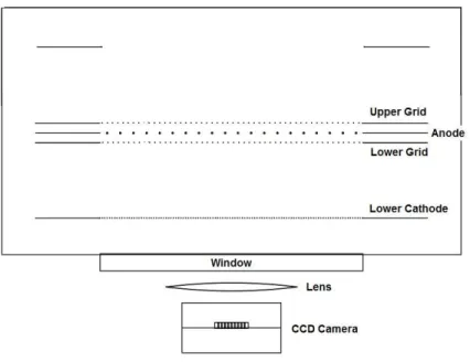
Figure 3.5: Schematics of our first TPC system. The electron drift region was only on the order of a couple centimeters with no field-shaping device. In order to avoid sparks, we started with fairly large amplification gap on the order of several millimeters at the sacrifice of the electron gain.
chamber is pumped down to low pressure, the impurities, mainly water, start coming out of the surface of the chamber and cause the detector gas inside to degrade. This is called outgassing. One can never achieve zero outgassing level; however, by pumping out for a long time or using the right material, the gas impurity level in the vacuum chamber was sufficiently low to allow data taking. Fig. 3.5 is the schematic of our very first R&D TPC system. The ground plate at bottom in the figure is no longer in use in our TPC system.
The dimensional specifications of the successful TPC prototype were as follows: anode frame was made with 100µm diameter wires at 5 mm of spacing, grid (ground) wires were made with 25 µm diameter wires at 2 mm of spacing to each other, and the cathode was made with mesh of 25µm stainless steel wires at 250µm pitch because there was very little difficulty in using mesh for the cathode; imperfection in stretching the mesh does not affect the integrity of the system. For this test, we used -1 kV for the cathode and +2.25 kV for the anode. The locations of the devices are shown in Fig. 3.5. The chamber was filled with
Figure 3.6: One of our very first optical images of an ion (α particle) travelling through low-pressure CF4 gas, and the scintillation due to the electron cascade captured by our CCD device. Theα particle starts from the top-right of the view to the bottom-left. Only a partial track is captured within the image because of the small field of view.
CF4 gas at 37 torr, which is in the range of gas pressure we are interested in the search for Dark Matter. Due to the limited quality of the CCD camera and gain available from our very first TPC amplification system, we had to place the lens as close to the amplification region as possible on the other side of the viewing port, so the actual viewing size was very small. Fig. 3.6 is the first image of an α particle track captured in our R&D prototype chamber, where the α particle was moving from right top to left bottom in the view. The CF4 gas purity level was essential for this successful optical measurement of theα particle tracks.
In Fig. 3.6, the actual size in scale is 2.5 cm horizontally and 1.7 cm vertically, and an electron multiplication gain reached on the order of 104. However, in order to have an ac-ceptable signal-to-noise ratio and capture clear images, software binning was necessary. A software binning is a method of combining neighboring multiple pixel information together in order to reach a higher gain at the sacrifice of spatial resolution. In this image, the actual image superpixel size was approximately 200 µm by 200 µm. In order to include
as many scintillation spots as possible, I rotated the CCD camera to an angle relative to the direction of the anode wires. In Fig. 3.6, the241Amα source was placed in such a way that theα particle traveled transverse to the direction of the anode wires. As mentioned earlier, the spacing of the anode wires was kept at 5 mm, so the distance between each scintillation spot in Fig. 3.6 was 5 mm.
When an α particle moved through gas inside the experimental chamber, it ionized the atoms along its path. If the particle traveled parallel to the direction of the wires, the ionization electrons scintillated along the wire, which was the path of the moving particle. On the other hand, if the particle moved perpendicular to the direction of the wires, it would leave pin points of the scintillation as shown in Fig. 3.6. Although the wire chamber worked beautifully, the spatial resolution of particle tracks was relatively poor. Also, the variation in wire spacing caused variations in gain; thus, it was very difficult to achieve good energy resolution. Furthermore, we did not have much knowledge about the purity of gas in the chamber at that point. However, we successfully captured signals fromα par-ticles optically. This proved that the fundamentals of our detection concept and method would work rather beautifully due to the robustness and simplicity of the detector, and the optical particle image readout by a CCD camera.
After the first success of capturing the αparticle track images with this wire chamber, we made an attempt to make a mesh anode plane. The basics of the design were the same, but with the mesh plane we could achieve much higher spatial resolution. This attempt turned out to be very challenging because we had no organized method of stretching out a mesh plane with equal tension in all directions. In order for the mesh plane to work, the gap distance in the amplification region had to be extremely small; otherwise, the cas-cade electrons would be spread out in much greater area compared to the wire chamber’s case, resulting in the lower electron gain per unit area. In order to overcome this problem and decrease the amplification distance gap, it was necessary to stretch out the mesh very
uniformly with greater tension. And at this point, we did not have a good method or knowledge of doing so. Thus, in parallel to continuing working on a mesh plane develop-ment, we pursued the wire plane readout method.
3.3
Prototype Dark Matter Detector at Boston University
3.3.1 First Wire Chamber Components
After our first success in proving the basics of our TPC detection mechanism, we began building our first prototype detector at Boston University (see Fig. 3.7). Our first task was to build what we had at MIT, but with improvement in quality and design. One example of the material selection was seeking out material with a low outgassing quality. In order to minimize outgassing of water vapor, the inner surface of the vacuum chamber from Kurt J. Lesker, Co. was electropolished. The TPC components were made out of aluminum or stainless steel plates as much as possible, and the wires were glued directly onto the aluminum frames with an inner opening of 20 cm by 20 cm with a thickness of 1.6 mm (see Fig. 3.8). We glued the wires onto the frame with 3M’s DP460EG low outgassing epoxy. This epoxy cures at room temperature over 24 hours and has sufficient strength to hold the wires in place. The wires were professionally stretched at Brookhaven National Lab (BNL) and glued onto an aluminum transfer frame of 48” by 52” (see Fig. 3.9). The frame and wires were returned to Boston University so that we could transfer the wires directly onto our own aluminum TPC frames (see Fig. 3.8). We had learned from our very first MIT R&D chamber about the importance of uniformity in spacing and tensioning of the wires, a uniformity which cannot be achieved by hand. With the wire winding machine at BNL, we had the wires stretched to a uniform tension of 100 g with a uniform spacing of 2.5 mm. For this operation, we used two different wires with different diameters; 50 µm gold-plated rhenium wire and 30µm gold-plated tungsten wire. With 100 g of tension, the natural sagging of the wires within the aluminum TPC frame due to gravity is minimal,
less than 2 µm for the Re-Au wire, and less than 1 µm for the W-Au wire. The breaking stress of the above wires is 600 g for the Re-Au wire and 200 g for the W-Au wire. In the amplification region, the electric field increases dramatically near the surface of the wire with a rate of inverse radius squared. We estimated that the electric field of greater than 106 v/m was required to have enough gain to view particle tracks. However, if the electric field becomes too great, the intense electric field is prone to the discharge problem. Any surface defect of the wires could cause the charges on the anode wires to find a path through gas onto the ground wires as a spark event. Thus, we had to be extremely careful and knowledgeable about the surface condition of the wires.
In a new design for the BU prototype experimental chamber, we employed the 50 µm diameter Re-Au wire with 7.5 mm spacing for the anode plane so that each wire would have enough gain but at the sacrifice of spatial resolution. Then the gap distance of the anode and grid (amplification region) was kept at 5 mm with the choice of the W-Au wires at 2.5 mm of wire pitches as the grid plane. We also used another W-Au wire plane as cathode, which was 25 mm away from the grid, creating 1 liter of sensitive volume. The wires of both grid and cathode planes were left with the spacing of 2.5 mm. In order to double the fiducial volume of the detector, we placed both grid and cathode layers on both sides with the anode layer in the middle just like the mirror image of the sensitive region on both sides of the anode plane (see Fig. 3.10).
The first CCD camera for this Boston University prototype chamber was an Apogee U2ME, which was equipped with a Kodak KAF-1603ME chip of 1536 by 1024 pixels with the size of 9 µm by 9µm. Each CCD pixel was also specially customized with micro lenses over the chip itself to enhance the light collection efficiency. By this, the quantum efficiency of the chip became nearly 80 % in the red region which we are interested in (see Fig. 3.11(a)). Initially a Schneider Xenon 0.95/17 lens was used to view the entire section of the am-plification region, but later we also tested a Schneider 0.95/25 lens in order to be able to
Figure 3.7: BU prototype TPC equipped with a CCD (bottom) and PMT (side). We use an Adixen Drytel 1025 pump (ATH 31+ turbomolecular pump and a AMD 1 roughout pump) to minimize any possible impurity introduced back into the chamber. This pump uses no lubrication in its parts.
(a) (b)
Figure 3.8: The BNL wires have been transferred to the aluminum frames of 20 cm by 20 cm openings.
(a) (b)
Figure 3.9: Stretched 50µm and 30µm wires attached to the transfer frame made at BNL. They used a special wire-winding machine made for the ATLAS experiment.
Figure 3.10: Schematic of the BU prototype R&D Dark Matter detector wire system. collect more light. The CCD camera is attached to the prototype chamber in such a way that the distance between the anode plane and CCD mounting surface is 309 mm. With the Schneider 17 mm lens attached to the CCD in the above setting, the spatial resolution of the image is 100µm per pixel. This is a very good resolution considering the length of typical nuclear recoil expected to be on the order of millimeters, although it turned out the gain was not very good so that we had to use a software binning of the CCD image pixels, and it was feasible because of the initial good spatial resolution of our detector.
Another new attempt we made on this prototype chamber is the use of a PMT in order to measure the timing of the particle tracks, which would enable us to obtain vertical infor-mation on each track. All the particle tracks captured by a CCD camera are 2D images projected onto the anode plane. Thus, it is not possible to identify if any particular par-ticle track has a vertical inclination or not. The PMT we used initially was Hamamatsu H1161-50. This PMT has quantum efficiency of roughly 5 % at the red region which is typical from CF4 scintillation (see Fig. 3.11(b)). With the initial design of the
experimen-(a) (b)
Figure 3.11: (a) Quantum efficiency curve for the Kodak KAF-1603ME CCD chip (East-man Kodak Company). (b) Quantum efficiency of Hamamatsu H1161 PMT (Kaboth et al., 2008).
tal chamber, there was no space to squeeze in this PMT next to the CCD camera on the other side of the viewing port. So we had to design a separate light path bent 90◦ onto another viewing port that was attached to the upper half of the experimental chamber (see Fig. 3.12(a)). The path bending mirror used for this operation is Edmund Optics NT47-110 (see Fig. 3.12(b)), with the surface plated with gold for superior efficiency of optical reflection and stability of surface quality in the CF4 gas. The PMT was installed so that the sensitive area of the PMT comes to the focal point of the mirror.
Although this attempt of the dual readout system was successful (see Fig. 3.13), in that we could prove our basic idea of dual readout by CCD and PMT, we found it difficult to identify how much light from each track was actually being captured by the PMT de-pending on their location. The pressure of CF4 gas in experiments at this point was set to 80 torr, which kept a good balance between enough track length and a low spark rate.
(a) (b)
Figure 3.12: (a) Schematics of the BU prototype TPC (Wellenstein and Dushkin). The Hamamatsu PMT was attached to the side window of the upper chamber, where the Apogee Alta U2ME CCD was attached to the bottom of the chamber, looking up towards the amplification region (see Fig. 3.7). (b) The wire-frame system and the mirror for PMT that go inside the prototype TPC.
(a) (b)
Figure 3.13: Example of anαtrack in 80 torr CF4gas travelling perpendicular to the anode wires. The images captured by (a) Apogee Alta U2ME, and (b) Hamamatsu H1161-50 PMT. The CCD image’s field of view is 15 cm by 10 cm. Each scintillation spot is separated by 7.5 mm to each other due to the anode wire spacing. Theα source was placed at 8 cm below the image, aiming towards the top of the figure. The CCD captured only part of theα track, where the PMT captured the whole track’s scintillation event.
It is in general more advantageous to increase the pressure in order to achieve higher gain by applying higher voltage onto the anode. However, as mentioned earlier, increasing the gas pressure reduces the track’s length-vs.-width ratio, thus compromising the detector’s directional sensitivity as a Dark Matter detector. Finding a good balance between the applied anode voltage and the detector gas pressure was without doubt one of the most challenging issues we had to overcome during the development of the detector.
The next step for improving the BU prototype Dark Matter detector was the introduction of the electron field cage in the drift region (see Fig. 3.14). In order to increase the sen-sitive volume, one has to move back the cathode mesh without hurting the uniformity of
the drift electric field. Since our first success at capturing the particle tracks in the pro-totype chamber, we have been studying and designing a field cage that will keep the drift electric field uniform inside and will not distort the particle tracks captured away from the amplification region. Considering the location of the PMT window and the dimension and distance between the CCD and amplification region, we designed a field cage of 20 cm in height, with field shaping rings spaced by 1 cm of spacing from each other. By installing the field-shaping cage, the sensitive volume of this chamber has now increased to 8 liters. On top of that, this enabled us to start learning about the transverse diffusion problem of particle tracks in a long electron drift distance that we must overcome in order to achieve our goal of identifying Dark Matter-induced nuclear recoils. The voltages of each field cage ring were set with a long resistive voltage divider chain. Since each resistor in the chain was 1 MΩ, the voltage dropped uniformly between cathode and ground.
3.3.2 Improvement to Mesh Chamber
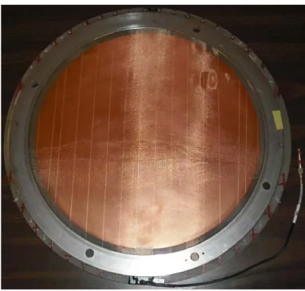
At this point, we had come to realize the limit of using wire frames as the anode and grid planes. Although it was very successful in capturing the image of the ion trajectory and demonstrating the feasibility of our technique, to learn more about the energy and length of the particle tracks captured by a CCD, we needed to improve the spatial resolution of the image. At the end of 2007, Denis Dujmic, our collaborator from MIT, succeeded in stretching the mesh evenly so that we could start using the mesh plane (see Fig. 3.15) instead of the wire plane that we had been working with. This improved the spatial reso-lution of the particle tracks dramatically but with some loss of light level per pixel because the particle tracks’ scintillation was scattered more to additional pixel locations. The mesh used in this construction is made with 80 % transparent stainless steel of 25µm wires at 250 µm pitch. A regular fluorocarbon fishing wire with diameter of 538 µm at a spacing of 2 cm was used to separate the grid mesh plane from the copper anode plane which was plated on the surface of a regular G-10 board. The same mesh was used to construct a
Figure 3.14: 20 cm long field-shaping cage for the electron drift region. Each ring is made out of SS304 with thickness of 1.6 mm, and inner diameter of 30 cm. A regular acrylic was used for spacers placed between