Bad Beta, Good Beta

(1)

H

I

E

R

Harvard Institute of Economic Research

Discussion Paper Number 2016

Bad Beta, Good Beta

by

John Y. Campbell

and

Tuomo Vuolteenaho

August 2003

Harvard University

Cambridge, Massachusetts

This paper can be downloaded without charge from:

http://post.economics.harvard.edu/hier/2003papers/2003list.html

(2)

Bad Beta, Good Beta

John Y. Campbell and Tuomo Vuolteenaho1

First draft: August 2002 This draft: August 2003

1_{Department of Economics, Littauer Center, Harvard University, Cambridge MA 02138, USA,}

and NBER. Email [email protected] and [email protected]. We would like to thank Michael Brennan, Joseph Chen, Randy Cohen, Robert Hodrick, Matti Keloharju, Owen Lamont, Greg Mankiw, Lubos Pastor, Antti Petajisto, Christopher Polk, Jay Shanken, Andrei Shleifer, Jeremy Stein, Sam Thompson, Luis Viceira, and seminar participants at Chicago GSB, Harvard Business School, the Kellogg School, and the NBER Asset Pricing meeting for helpful comments. We are grateful to Ken French for providing us with some of the data used in this study. All errors and omissions remain our responsibility. This material is based upon work supported by the National Science Foundation under Grant No. 0214061 to Campbell.

(3)

Abstract

This paper explains the size and value “anomalies” in stock returns using an economically motivated two-beta model. We break the CAPM beta of a stock with the market portfolio into two components, one reflecting news about the market’s future cashflows and one reflecting news about the market’s discount rates. Intertemporal asset pricing theory suggests that the former should have a higher price of risk; thus beta, like cholesterol, comes in “bad” and “good” varieties. Empirically, wefind that value stocks and small stocks have considerably higher cash-flow betas than growth stocks and large stocks, and this can explain their higher average returns. The poor performance of the CAPM since 1963 is explained by the fact that growth stocks and high-past-beta stocks have predominantly good betas with low risk prices.

(4)

1

Introduction

How should a rational investor measure the risks of stock market investments? What determines the risk premium that will induce a rational investor to hold an individual stock at its market weight, rather than overweighting or underweighting it? Accord-ing to the Capital Asset PricAccord-ing Model (CAPM) of Sharpe (1964) and Lintner (1965), a stock’s risk is summarized by its beta with the market portfolio of all invested wealth. Controlling for beta, no other characteristics of a stock should influence the return required by a rational investor.

It is well known that the CAPM fails to describe average realized stock returns since the early 1960’s, if a value-weighted equity index is used as a proxy for the market portfolio. In particular, small stocks and value stocks have delivered higher average returns than their betas can justify. Adding insult to injury, stocks with high past betas have had average returns no higher than stocks of the same size with low past betas. Thesefindings tempt investors to tilt their stock portfolios systematically towards small stocks, value stocks, and stocks with low past betas.2

We argue that returns on the market portfolio have two components, and that recognizing the diﬀerence between these two components can eliminate the incentive to overweight value, small, and low-beta stocks. The value of the market portfolio may fall because investors receive bad news about future cashflows; but it may also fall because investors increase the discount rate or cost of capital that they apply to these cash flows. In the first case, wealth decreases and investment opportunities are unchanged, while in the second case, wealth decreases but future investment opportunities improve.

These two components should have diﬀerent significance for a risk-averse, long-term investor who holds the market portfolio. Such an investor may demand a higher premium to hold assets that covary with the market’s cash-flow news than to hold assets that covary with news about the market’s discount rates, for poor returns driven by increases in discount rates are partially compensated by improved prospects for future returns. To properly measure risk for this investor, the single

2_{Seminal early references include Banz (1981) and Reinganum (1981) for the size e}_ﬀ_{ect, and}

Graham and Dodd (1934), Basu (1977, 1983), Ball (1978), and Rosenberg, Reid, and Lanstein (1985) for the value eﬀect. Fama and French (1992) give an influential treatment of both eﬀects within an integrated framework and show that sorting stocks on past market betas generates little variation in average returns.

(5)

beta of the Sharpe-Lintner CAPM should be broken into two diﬀerent betas: a

cash-flow beta and a discount-rate beta. We expect a rational investor who is holding the market portfolio to demand a greater reward for bearing the former type of risk than the latter. In fact, an intertemporal capital asset pricing model (ICAPM) of the sort proposed by Merton (1973) suggests that the the price of risk for the discount-rate beta should equal the variance of the market return, while the price of risk for the cash-flow beta should be γ times greater, where γ is the investor’s coeﬃcient of relative risk aversion. If the investor is conservative in the sense that γ > 1, the cash-flow beta has a higher price of risk.

An intuitive way to summarize our story is to say that beta, like cholesterol, has a “bad” variety and a “good” variety. The required return on a stock is determined not by its overall beta with the market, but by its bad cash-flow beta and its good discount-rate beta. Of course, the good beta is good not in absolute terms, but in relation to the other type of beta.

We test these ideas by fitting a two-beta ICAPM to historical monthly returns on stock portfolios sorted by size, book-to-market ratios, and market betas. We consider not only a sample period since 1963 that has been the subject of much recent research, but also an earlier sample period 1929-1963 using the data of Davis, Fama, and French (2000). In the modern period, 1963:7-2001:12, we find that the two-beta model greatly improves the poor performance of the standard CAPM. The main reason for this is that growth stocks, with low average returns, have high betas with the market portfolio; but their high betas are predominantly good betas, with low risk prices. Value stocks, with high average returns, have higher bad betas than growth stocks do. In the early period, 1929:1-1963:6, we find that value stocks have higher CAPM betas and proportionately higher bad betas than growth stocks, so the single-beta CAPM adequately explains the data.

The ICAPM also explains the size effect. Over both subperiods, small stocks outperform large stocks by approximately 3% per annum. In the early period, this performance differential is justified by the moderately higher cash-flow and discount-rate betas of small stocks relative to large stocks. In the modern period, small and large stocks have approximately equal cash-flow betas. However, small stocks have much higher discount-rate betas than large stocks in the post-1963 sample. Even though the premium on discount-rate beta is low, the magnitude of the beta spread is sufficient to explain most of the size premium.

(6)

show a spread in average returns in the early sample period but not in the modern period. In the early sample period, a sort on CAPM beta induces a strong post-ranking spread in cash-flow betas, and this spread carries an economically significant premium, as the theory predicts. In the modern period, however, sorting on past CAPM betas produces a spread only in good discount-rate betas but no spread in bad cash-flow betas. Since the good beta carries only a low premium, the almostflat relation between average returns and the CAPM beta estimated from these portfolios in the modern period is no puzzle to the two-beta model.

All these findings are based on the first-order condition of a long-term investor who is assumed to hold a value-weighted stock market index. We show that there exists a coefficient of risk aversion that makes the investor content to hold equities at their value weights, rather than systematically tilting her portfolio towards value stocks, small stocks, or stocks with low past betas. For an investor with this degree of risk aversion, the high average returns on such stocks are appropriate compensation for their risks in relation to the value-weighted index. An investor with a lower risk aversion coefficient would find value, small, and low-past-beta stocks attractive and would wish to overweight them, while an investor with a higher risk aversion coefficient would wish to underweight these stocks.

Our model explains why stocks with high cash-flow betas may offer high average returns, given that long-term investors are fully invested in equities at all times, or, in a slight generalization of the model, maintain a constant allocation to equities. Our model does not explain why long-term investors would wish to keep their equity allocations constant. If the equity premium is time-varying, it is optimal for a long-term investor with afixed coefficient of relative risk aversion to invest more in equities at times when the equity premium is high (Campbell and Viceira 1999, Kim and Omberg 1996). We could generalize the model to allow a time-varying equity weight in the investor’s portfolio, but this would not be consistent with general equilibrium if all investors have the same preferences. Thus our model cannot be interpreted as a representative agent general equilibrium model of the economy. Our achievement is merely to show that the prices of risk for value, small, and low-past-beta stocks are sufficient to deter investment in these stocks by conservative long-term investors who eschew market timing.

In developing and testing the two-beta ICAPM, we draw on a great deal of re-lated literature. The idea that the market’s return can be attributed to cash-flow and discount-rate news is not novel. Campbell and Shiller (1988a) develop a

(7)

loglin-ear approximate framework in which to study the eﬀects of changing cash-flow and discount-rate forecasts on stock prices. Campbell (1991) uses this framework and a vector autoregressive (VAR) model to decompose market returns into cash-flow news and discount-rate news. Empirically, he finds that discount-rate news is far from negligible; in postwar US data, for example, his VAR system explains most stock return volatility as the result of discount-rate news. Campbell and Mei (1993) use a similar approach to decompose the market betas of industry and size portfolios into cash-flow betas and discount-rate betas, but they do not estimate separate risk prices for these betas.

The insight that long-term investors care about shocks to investment opportu-nities is due to Merton (1973). Campbell (1993) solves a discrete-time empirical version of Merton’s ICAPM, assuming that asset returns are homoskedastic and that a representative investor has the recursive preferences proposed by Epstein and Zin (1989, 1991). The solution is exact in the limit of continuous time if the representa-tive investor has elasticity of intertemporal substitution equal to one, and is otherwise a loglinear approximation. Campbell writes the solution in the form of a K-factor model, where the first factor is the market return and the other factors are shocks to variables that predict the market return. Campbell (1996) also tests this model on industry portfolios, but finds that in his specification the innovation to discount rates is highly correlated with the innovation to the market itself; thus his multi-beta model is hard to distinguish empirically from the CAPM. Li (1997), Hodrick, Ng, and Sengmueller (1999), Lynch (1999), Brennan, Wang, and Xia (2001, 2003), Ng (2002), Guo (2002), and Chen (2003) also explore the empirical implications of Merton’s model.

The two papers that are closest to ours in their focus are Brennan, Wang, and Xia (2003) and Chen (2003). Brennan et al. model the riskless interest rate and the Sharpe ratio on the market portfolio as continuous-time AR(1) processes. They estimate the parameters of their model using bond market data, and explore the model’s implications for the value and size eﬀects in US equities since 1953. They have some success in explaining these eﬀects, but they do not relate the risk prices for interest rate and Sharpe ratio shocks to the underlying preferences of investors. Chen (2003) extends the framework of Campbell (1993) to allow for heteroskedastic asset returns, and estimates a VAR-GARCH model to describe the dynamics of stock returns. Given the variables he includes in his model, he finds little evidence that growth stocks are valuable hedges against shocks to investment opportunities.

(8)

Recently, however, several authors have found that high returns to growth stocks, particularly small growth stocks, seem to predict low returns on the aggregate stock market. Eleswarapu and Reinganum (2003) use lagged 3-year returns on an equal-weighted index of growth stocks, while Brennan, Wang, and Xia (2001) use the dif-ference between the log book-to-market ratios of small growth stocks and small value stocks to predict the aggregate market. In this paper we use a measure similar to that of Brennan et al. (2001) and find that indeed growth stock returns have high covariances with declines in market discount rates.

It is natural to ask why high returns on small growth stocks should predict low returns on the stock market as a whole. This is a particularly important question since time-series regressions of aggregate stock returns on arbitrary predictor variables can easily produce meaningless data-mined results. One possibility is that small growth stocks generate cash flows in the more distant future and therefore their prices are more sensitive to changes in discount rates, just as coupon bonds with a high duration are more sensitive to interest-rate movements than are bonds with a low duration (Cornell 1999). Another possibility is that small growth companies are particularly dependent on external financing and thus are sensitive to equity market and broader financial conditions (Ng, Engle, and Rothschild 1992, Perez-Quiros and Timmermann 2000). A third possibility is that episodes of irrational investor optimism (Shiller 2000) have a particularly powerful eﬀect on small growth stocks.

Our finding that value stocks have higher cash-flow betas than growth stocks is consistent with the empirical results of Cohen, Polk, and Vuolteenaho (2002). Cohen et al. measure cash-flow betas by regressing the multi-year return on equity (ROE) of value and growth stocks on the market’s multi-year ROE. Theyfind that value stocks have higher ROE betas than growth stocks. There is also evidence that value stock returns are correlated with shocks to GDP-growth forecasts (Liew and Vassalou 2000, Vassalou 2003). These empirical findings are consistent with Brainard, Shapiro, and Shoven’s (1991) suggestion that “fundamental betas” estimated from cashflows could improve the empirical performance of the CAPM. This sensitivity of value stocks’ cash-flow fundamentals to economy-wide cash-flow fundamentals plays a key role in our two-beta model’s ability to explain the value premium.

There are numerous competing explanations for the size and value eﬀects. At the most basic level the Arbitrage Pricing Theory (APT) of Ross (1976) allows any pervasive source of common variation to be a priced risk factor. Fama and French

(9)

(1993) show that small stocks and value stocks tend to move together as groups, and introduce an influential three-factor model, including a market factor, size factor, and value factor, to describe the size and value eﬀects in average returns. As Fama and French recognize, ultimately this falls short of a satisfactory explanation because the APT is silent about what determines factor risk prices; in a pure APT model the size premium and the value premium could just as easily be zero or negative.

Jagannathan and Wang (1996) point out that the CAPM might hold conditionally, but fail unconditionally. If some stocks have high market betas at times when the market risk premium is high, then these stocks should have higher average returns than are explained by their unconditional market betas. Lettau and Ludvigson (2001) and Zhang and Petkova (2002) argue that value stocks satisfy these conditions, although Lewellen and Nagel (2003) argue that time-varying betas cause only a very modest increase in average returns.

Adrian and Franzoni (2002) and Lewellen and Shanken (2002) consider the pos-sibility that investors do not know the risk characteristics of stocks but must learn about them over time. Adrian and Franzoni, for example, suggest that investors tended to overestimate the market betas of value and small stocks as these betas trended downwards during the 20th Century. This led investors to demand higher average returns for such stocks than are justified by their average market risks.

Roll (1977) emphasizes that tests of the CAPM are misspecified if one cannot measure the market portfolio correctly. While Stambaugh (1982) and Shanken (1987)

find that CAPM tests are insensitive to the inclusion of other financial assets, more recent research has stressed the importance of human wealth whose return can be proxied by revisions in expected future labor income (Campbell 1996, Jagannathan and Wang 1996, Lettau and Ludvigson 2001).

Finally, the value eﬀect can also be interpreted in behavioral terms. Lakonishok, Shleifer, and Vishny (1994), for example, argue that investors irrationally extrapolate past earnings growth and thus overvalue companies that have performed well in the past. These companies have low book-to-market ratios and subsequently underper-form once their earnings growth disappoints investors. Supporting evidence is pro-vided by La Porta (1996), who shows that high long-term earnings forecasts of stock market analysts predict low stock returns while low forecasts predict high returns, and by La Porta et al. (1997), who show that the underperformance of stocks with low book-to-market ratios is concentrated on earnings announcement dates. Brav, Lehavy, and Michaely (2002) show that analysts’ price targets imply high

(10)

subjec-tive expected returns on growth stocks, consistent with the hypothesis that the value eﬀect is due to expectational errors.

In this paper we do not consider any of these alternative stories. We assume that unconditional betas are adequate proxies for conditional betas, we use a value-weighted index of common stocks as a proxy for the market portfolio, and we test an orthodox asset pricing model based on thefirst-order conditions of a rational investor who knows the parameters of the model. Our purpose is to clarify the extent to which deviations from the CAPM’s cross-sectional predictions can be rationalized by Merton’s (1973) intertemporal hedging considerations that are relevant for long-term investors. This exercise should be of interest even if one believes that investor irrationality has an important eﬀect on stock prices, because even in this case one should want to know how a rational investor will perceive stock market risks. Our analysis has obvious relevance to long-term institutional investors such as pension funds, which maintain stable allocations to equities and wish to assess the risks of tilting their equity portfolios towards particular types of stocks.

The organization of the paper is as follows. In Section 2, we estimate two com-ponents of the return on the aggregate stock market, one caused by cash-flow shocks and the other by discount-rate shocks. In Section 3, we use these components to estimate cash-flow and discount-rate betas for portfolios sorted onfirm characteristics and risk loadings. In Section 4, we lay out the intertemporal asset pricing theory that justifies different risk premia for bad cash-flow beta and good discount-rate beta. We also show that the returns to small and value stocks can largely be explained by allowing different risk premia for these two different betas. Section 5 concludes.

2

How cash-

fl

ow and discount-rate news move the

market

A simple present-value formula points to two reasons why stock prices may change. Either expected cashflows change, discount rates change, or both. In this section, we empirically estimate these two components of unexpected return for a value-weighted stock market index. Consistent with findings of Campbell (1991), the fitted values suggest that over our sample period (1929:1-2001:12) discount-rate news causes much more variation in monthly stock returns than cash-flow news.

(11)

2.1

Return-decomposition framework

Campbell and Shiller (1988a) develop a loglinear approximate present-value relation that allows for time-varying discount rates. They do this by approximating the

de-finition of log return on a dividend-paying asset, rt+1 ≡ log(Pt+1+Dt+1)−log(Pt),

around the mean log dividend-price ratio, (dt−pt), using a first-order Taylor

ex-pansion. Above, P denotes price, D dividend, and lower-case letters log trans-forms. The resulting approximation is rt+1 ≈ k +ρpt+1 + (1−ρ)dt+1 −pt ,where

ρ and k are parameters of linearization defined by ρ _≡ 1±¡1 + exp(dt−pt) ¢

and k _{≡ −}log(ρ)₋(1₋ρ) log(1/ρ₋1). When the dividend-price ratio is constant, then ρ =P/(P +D), the ratio of the ex-dividend to the cum-dividend stock price. The approximation here replaces the log sum of price and dividend with a weighted aver-age of log price and log dividend, where the weights are determined by the averaver-age relative magnitudes of these two variables.

Solving forward iteratively, imposing the “no-infinite-bubbles” terminal condition that limj→∞ρj(dt+j −pt+j) = 0, taking expectations, and subtracting the current

dividend, one gets

pt−dt= k 1₋ρ + Et ∞ X j=0 ρj[∆dt+1+j−rt+1+j], (1)

where∆ddenotes log dividend growth. This equation says that the log price-dividend ratio is high when dividends are expected to grow rapidly, or when stock returns are expected to be low. The equation should be thought of as an accounting identity rather than a behavioral model; it has been obtained merely by approximating an identity, solving forward subject to a terminal condition, and taking expectations. Intuitively, if the stock price is high today, then from the definition of the return and the terminal condition that the dividend-price ratio is non-explosive, there must either be high dividends or low stock returns in the future. Investors must then expect some combination of high dividends and low stock returns if their expectations are to be consistent with the observed price.

While Campbell and Shiller (1988a) constrain the discount coeﬃcient ρto values determined by the average log dividend yield, ρ has other possible interpretations as well. Campbell (1993, 1996) links ρ to the average consumption-wealth ratio. In eﬀect, the latter interpretation can be seen as a slightly modified version of the former. Consider a mutual fund that reinvests dividends and a mutual-fund investor

(12)

who finances her consumption by redeeming a fraction of her mutual-fund shares every year. Eﬀectively, the investor’s consumption is now a dividend paid by the fund and the investor’s wealth (the value of her remaining mutual fund shares) is now the ex-dividend price of the fund. Thus, we can use (1) to describe a portfolio strategy as well as an underlying asset and let the average consumption-wealth ratio generated by the strategy determine the discount coeﬃcient ρ, provided that the consumption-wealth ratio implied by the strategy does not behave explosively.

Campbell (1991) extends the loglinear present-value approach to obtain a decom-position of returns. Substituting (1) into the approximate return equation gives

rt+1−Etrt+1 = (Et+1−Et) ∞ X j=0 ρj∆dt+1+j −(Et+1−Et) ∞ X j=1 ρjrt+1+j (2) = NCF,t+1−NDR,t+1,

whereNCF denotes news about future cashflows (i.e., dividends or consumption), and

NDR denotes news about future discount rates (i.e., expected returns). This equation

says that unexpected stock returns must be associated with changes in expectations of future cash flows or discount rates. An increase in expected future cash flows is associated with a capital gain today, while an increase in discount rates is associated with a capital loss today. The reason is that with a given dividend stream, higher future returns can only be generated by future price appreciation from a lower current price.

These return components can also be interpreted as permanent and transitory shocks to wealth. Returns generated by cash-flow news are never reversed subse-quently, whereas returns generated by discount-rate news are oﬀset by lower returns in the future. From this perspective it should not be surprising that conservative long-term investors are more averse to cash-flow risk than to discount-rate risk.

2.2

Implementation with a VAR model

We follow Campbell (1991) and estimate the cash-flow-news and discount-rate-news series using a vector autoregressive (VAR) model. This VAR methodologyfirst esti-mates the termsEtrt+1and(Et+1−Et)

P∞

j=1ρ

j_r

t+1+j and then usesrt+1and equation

(13)

does not necessarily have to understand the short-run dynamics of dividends. Un-derstanding the dynamics of expected returns is enough.

We assume that the data are generated by a first-order VAR model

zt+1 =a+Γzt+ut+1, (3)

wherezt+1 is am-by-1 state vector withrt+1 as its first element, a andΓ arem-by-1

vector and m-by-m matrix of constant parameters, and ut+1 an i.i.d. m-by-1 vector

of shocks. Of course, this formulation also allows for higher-order VAR models via a simple redefinition of the state vector to include lagged values.

Provided that the process in equation (3) generates the data, t+ 1 cash-flow and discount-rate news are linear functions of the t+ 1 shock vector:

NCF,t+1 = (e10+e10λ)ut+1 (4)

NDR,t+1 = e10λut+1.

The VAR shocks are mapped to news by λ, defined as λ _≡ ρΓ(I ₋ ρΓ)−1. e10λ captures the long-run significance of each individual VAR shock to discount-rate ex-pectations. The greater the absolute value of a variable’s coeﬃcient in the return prediction equation (the top row ofΓ), the greater the weight the variable receives in the discount-rate-news formula. More persistent variables should also receive more weight, which is captured by the term(I₋ρΓ)−1_.

2.3

VAR data

To operationalize the VAR approach, we need to specify the variables to be included in the state vector. We opt for a parsimonious model with the following four state variables. First, the excess log return on the market (re

M) is the diﬀerence between

the log return on the Center for Research in Securities Prices (CRSP) value-weighted stock index (rM) and the log risk-free rate. The risk-free-rate data are constructed

by CRSP from Treasury bills with approximately three month maturity.

Second, the term yield spread (T Y) is provided by Global Financial Data and is computed as the yield diﬀerence between ten-year constant-maturity taxable bonds and short-term taxable notes, in percentage points.

(14)

Third, the price-earnings ratio (P E) is from Shiller (2000), constructed as the price of the S&P 500 index divided by a ten-year trailing moving average of aggre-gate earnings of companies in the S&P 500 index. Following Graham and Dodd (1934), Campbell and Shiller (1988b, 1998) advocate averaging earnings over several years to avoid temporary spikes in the price-earnings ratio caused by cyclical declines in earnings. We avoid any interpolation of earnings in order to ensure that all com-ponents of the time-t price-earnings ratio are contemporaneously observable by time t. The ratio is log transformed.

Fourth, the small-stock value spread (V S) is constructed from the data made available by Professor Kenneth French on his web site.3 _{The portfolios, which are}

constructed at the end of each June, are the intersections of two portfolios formed on size (market equity, M E) and three portfolios formed on the ratio of book equity to market equity (BE/M E). The size breakpoint for yeartis the median NYSE market equity at the end of June of yeart. BE/M E for June of yeart is the book equity for the lastfiscal year end int₋1divided by M E for December of t₋1. The BE/M E breakpoints are the 30th and 70th NYSE percentiles.

At the end of June of year t, we construct the small-stock value spread as the diﬀerence between the log(BE/M E) of the small high-book-to-market portfolio and thelog(BE/M E)of the small low-book-to-market portfolio, whereBE andM E are measured at the end of December of year t₋1. For months from July to May, the small-stock value spread is constructed by adding the cumulative log return (from the previous June) on the small low-book-to-market portfolio to, and subtracting the cumulative log return on the small high-book-to-market portfolio from, the end-of-June small-stock value spread.

Our small-stock value spread is similar to variables constructed by Asness, Fried-man, Krail, and Liew (2000), Cohen, Polk, and Vuolteenaho (2003), and Brennan, Wang, and Xia (2001). Asness et al. use a number of diﬀerent scaled-price vari-ables to construct their measures, and also incorporate analysts’ earnings forecasts into their model. Cohen et al. use the entire CRSP universe instead of small-stock portfolios to construct their spread variable. Brennan et al.’s small-stock value-spread variable is equal to ours at the end of June of each year, but the intra-year values diﬀer because Brennan et al. interpolate the intra-year values of BE using year t and year t+ 1 BE values. We do not follow their procedure because we wish to avoid using any future variables that might cause spurious forecastability of stock

(15)

returns.

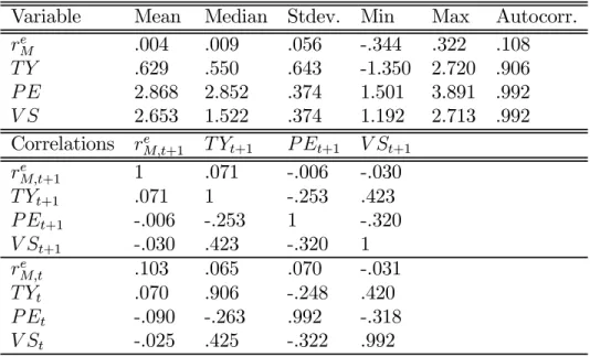
These state-variable series span the period 1928:12—2001:12. Table 1 shows de-scriptive statistics and Figure 1 the time-series evolution of the state variables, ex-cluding the market return. The variables in Figure 1 are demeaned and normalized by their sample standard deviation.

The black solid line in Figure 1 plots the evolution of P E, the log ratio of price to ten-year moving average of earnings. Our sample period begins only months before the stock market crash of 1929. This event is clearly visible from the graph in which the log price-earnings drops by an extraordinaryfive sample standard deviations from 1929 to 1932. Another striking episode is the 1983-1999 bull market, during which the price-earnings ratio increases by four sample standard deviations.

While the price-earnings ratio and its historical time-series behavior are well known, the history of the small-stock value spread is perhaps less so. Recall that our value-spread variable is the diﬀerence between value stocks’ log book-to-market ratio and growth stocks’ log book-to-market ratio. Thus a high value spread is associated with high prices for growth stocks relative to value stocks. Similar to figures shown by Cohen, Polk, and Vuolteenaho (2003) and Brennan, Wang, and Xia (2001), the post-war variation in V S appears positively correlated with the price-earnings ra-tio, high overall stock prices coinciding with especially high prices for growth stocks. The pre-war data appear quite diﬀerent from the post-war data, however. For the

first two decades of our sample, the value spread is negatively correlated with the market’s price-earnings ratio. The correlation between V S and P E is -.48 in the period 1928:12—1963:6, and .57 in the period 1963:7—2001:12. If most value stocks were highly levered andfinancially distressed during and after the Great Depression, it makes sense that their values were especially sensitive to changes in overall eco-nomic prospects, including the cost of capital. In the post-war period, however, most value stocks were probably stable businesses with relatively lowfinancial leverage, no growth options, and thus probably little dependence on external equity-market fi -nancing. We will return to this changing sensitivity of value and growth stocks to various economy-wide shocks in Section 3.

The term yield spread (T Y) is a variable that is known to track the business cycle, as discussed by Fama and French (1989). The term yield spread is very volatile during the Great Depression and again in the 1970’s. It also tracks the value spread closely, with a correlation of .42 over the full sample as shown in Table 1. Because long-bond yields are relatively stable, T Y is mostly driven by the volatile short end of the term

(16)

structure, making the variable negatively correlated with the overall level of interest rates. Since growth stocks are assets with a high duration, as emphasized by Cornell (1999), it is not surprising that high prices for growth stocks coincide with low interest rates and thus a high term yield spread.

2.4

VAR parameter estimates

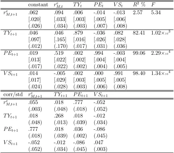
Table 2 reports parameter estimates for the VAR model. Each row of the table corre-sponds to a different equation of the model. Thefirstfive columns report coefficients on the five explanatory variables: a constant, and lags of the excess market return, term yield spread, price-earnings ratio, and small-stock value spread. OLS standard errors are reported in square brackets below the coefficients. For comparison, we also report in parentheses standard errors from a bootstrap exercise. Finally, we report theR2 andF statistics for each regression. The bottom of the table reports the cor-relation matrix of the equation residuals, with standard deviations of each residual on the diagonal.

The first row of Table 2 shows that all four of our VAR state variables have some ability to predict excess returns on the aggregate stock market. Market returns display a modest degree of momentum; the coeﬃcient on the lagged excess market return is .094 with a standard error of .034. The term yield spread positively pre-dicts the market return, consistent with thefindings of Keim and Stambaugh (1986), Campbell (1987), and Fama and French (1989). The smoothed price-earnings ratio negatively predicts the return, consistent with Campbell and Shiller (1988b, 1998) and related work using the aggregate dividend-price ratio (Rozeﬀ1984, Campbell and Shiller 1988a, and Fama and French 1988, 1989). The small-stock value spread neg-atively predicts the return, consistent with Eleswarapu and Reinganum (2003) and Brennan, Wang, and Xia (2001). Overall, the R2 _{of the return forecasting equation}

is about 2.6%, which is a reasonable number for a monthly model.

The remaining rows of Table 2 summarize the dynamics of the explanatory vari-ables. The term spread is approximately an AR(1) process with an autoregressive coeﬃcient of .88, but the lagged small-stock value spread also has some ability to predict the term spread. This should not be surprising given the contemporaneous correlation of these two variables illustrated in Figure 1. The price-earnings ratio is highly persistent, with a root very close to unity, but it is also predicted by the lagged market return. This predictability may reflect short-term momentum in stock

(17)

returns, but it may also reflect the fact that the recent history of returns is correlated with earnings news that is not yet reflected in our lagged earnings measure. Finally, the small-stock value spread is also a highly persistent AR(1) process.

The persistence of the VAR explanatory variables raises some difficult statistical issues. It is well known that estimates of persistent AR(1) coefficients are biased downwards in finite samples, and that this causes bias in the estimates of predictive regressions for returns if return innovations are highly correlated with innovations in predictor variables (Stambaugh 1999). There is an active debate about the effect of this on the strength of the evidence for return predictability (Ang and Bekaert 2001, Campbell and Yogo 2002, Lewellen 2003, Torous, Valkanov, and Yan 2003).

For our sample and VAR specification, the four predictive variables in the return prediction equation are jointly significant at a better than 5% level. Our unreported experiments show that the joint significance of the return-prediction equation at 5% level survives bootstrapping excess returns as return shocks and simulating from a system estimated under the null with various bias adjustments. However, the statistical significance of the one-period return-prediction equation does not guarantee that our news terms are not materially aﬀected by the above-mentioned small-sample bias.

As a simple way to assess the impact of this bias, we have generated 2500 artificial data series using the estimated VAR coefficients and have reestimated the VAR system 2500 times. The difference between the average coefficient estimates in the artificial data and the original VAR estimates is a simple measure offinite-sample bias. Wefind that there is some bias in the VAR coefficients, but it does not have a large effect on our estimates of cash-flow and discount-rate news. The reason is that the bias causes some overstatement of short-term return predictability (thee10ρΓcomponent ofe10λ) but an understatement of the persistence of the VAR, and thus an understatement of the long-term impact of predictability [the(I₋ρΓ)−1 _{component of}_e₁0_{λ]. These two}

eﬀects work against each other. The one variable that is moderately aﬀected by bias is the value spread, whose role in predicting returns is biased downwards. Since this bias works against us in explaining the average returns on value and growth stocks, we do not attempt to correct it. Instead we use the estimated VAR as a reasonable representation of the data and ask what it implies for cross-sectional asset pricing puzzles, and for risks relevant to a long-horizon investor.

Table 3 summarizes the behavior of the implied cash-flow news and discount-rate news components of the market return. The top panel shows that discount-rate

(18)

news has a standard deviation of about 5% per month, much larger than the 2.5% standard deviation of cash-flow news. This is consistent with thefinding of Campbell (1991) that discount-rate news is the dominant component of the market return. The table also shows that the two components of return are almost uncorrelated with one another. Thisfinding diﬀers from Campbell (1991) and particularly Campbell (1996); it results from our use of a richer forecasting model that includes the value spread as well as the aggregate price-earnings ratio.

Table 3 also reports the correlations of each state variable innovation with the es-timated news terms, and the coeﬃcients(e10₊_e₁0_λ₎ _and _e₁0_λ _{that map innovations}

to cash-flow and discount-rate news. Innovations to returns and the price-earnings ratio are highly negatively correlated with discount-rate news, reflecting the mean reversion in stock prices that is implied by our VAR system. Market return innova-tions are weakly positively correlated with cash-flow news, indicating that some part of a market rise is typically justified by underlying improvements in expected future cashflows. Innovations to the price-earnings ratio, however, are weakly negatively correlated with cash-flow news, suggesting that price increases relative to earnings are not usually justified by improvements in future earnings growth.

Figure 2 illustrates the VAR model’s view of stock market history in relation to NBER recessions. Each dotted line in the figure corresponds to the trough of a recession as defined by the NBER. The top panel reports a trailing exponentially-weighted moving average of the market’s cash-flow news, while the bottom panel reports the same moving average of the market’s discount-rate news. It is clear from thefigure that in some recessions our model attributes stock market declines to declining cash flows (e.g. 1991), in others to increasing discount rates (e.g. 2001), and in others to both types of news (e.g. the Great Depression and the 1970’s). We might call the first type of recession a “profitability recession”, the second type a “valuation recession”, and the third type a “mixed recession”. A valuation recession is characterized by a declining price-earnings ratio, a steepening yield curve, and larger declines in growth stocks than in value stocks. Profitability and valuation recessions, as opposed to mixed recessions, will be particularly influential observations when we estimate cash-flow and discount-rate betas, because these are episodes in which cash-flow and discount-rate news do not move closely together.

We setρ=.951/12_{in Table 3 and use the same value throughout the paper. Recall}

thatρcan be related to either the average dividend yield or the average consumption wealth ratio, as discussed on page 8. An annualizedρof .95 corresponds to an average

(19)

dividend-price or consumption-wealth ratio of -2.94 (in logs) or 5.2% (in levels), where wealth is measured after subtracting consumption. We picked the value .95 because approximately 5% consumption of the total wealth per year seems reasonable for a long-term investor, such as a university endowment.

As a robustness check, we have estimated the VAR over subsamples before and after 1963. The coefficients that map state variable innovations to cash-flow and discount-rate news are fairly stable, with no changes in sign. Also, the value spread has greater predictive power in the first subsample than in the second. This is reassuring, since it indicates that the coefficient on this variable is not justfitting the last few years of the sample during which exceptionally high prices for growth stocks preceded a market decline. Given the stability of the VAR point estimates in the two subsamples and the unfortunate statistical fact that the coefficients of our monthly return-prediction regressions are estimated imprecisely (a problem that is magnified in shorter subsamples), we proceed to use the full-sample VAR-coefficient estimates in the remainder of the paper.

3

Measuring cash-

fl

ow and discount-rate betas

We have shown that market returns contain two components, both of which display substantial volatility and which are not highly correlated with one another. This raises the possibility that diﬀerent types of stocks may have diﬀerent betas with the two components of the market. In this section we measure cash-flow betas and discount-rate betas separately. We define the cash-flow beta as

β_i,CF _≡ Cov (ri,t, NCF,t)

Var¡re

M,t−Et−1reM,t

¢ (5)

and the discount-rate beta as

βi,DR ≡

Cov (ri,t,−NDR,t)

Var¡re

M,t−Et−1reM,t

¢. (6)

Note that the discount-rate beta is defined as the covariance of an asset’s return withgood news about the stock market in form oflower-than-expected discount rates, and that each beta divides by the total variance of unexpected market returns, not

(20)

the variance of cash-flow news or discount-rate news separately. This implies that the cash-flow beta and the discount-rate beta add up to the total market beta,

βi,M =βi,CF +βi,DR. (7)

Our estimates show that there is interesting variation across assets and across time in the two components of the market beta.

3.1

Test-asset data

We construct two sets of portfolios to use as test assets. Thefirst is a set of 25M E and BE/M E portfolios, available from Professor Kenneth French’s web site. The portfolios, which are constructed at the end of each June, are the intersections offive portfolios formed on size (M E) and five portfolios formed on book-to-market equity (BE/M E). BE/M E for June of year t is the book equity for the last fiscal year end in the calendar year t₋1 divided by M E for December of t₋1. The size and BE/M E breakpoints are NYSE quintiles. On a few occasions, nofirms are allocated to some of the portfolios. In those cases, we use the return on the portfolio with the same size and the closestBE/M E.

The 25 M E andBE/M E portfolios were originally constructed by Davis, Fama, and French (2000) using three databases. Thefirst of these, the CRSP monthly stock

file, contains monthly prices, shares outstanding, dividends, and returns for NYSE, AMEX, and NASDAQ stocks. The second database, the COMPUSTAT annual research file, contains the relevant accounting information for most publicly traded U.S. stocks. The COMPUSTAT accounting information is supplemented by the third database, Moody’s book equity information hand collected by Davis et al.

Daniel and Titman (1997) point out that it can be dangerous to test asset pricing models using only portfolios sorted by characteristics known to be related to average returns, such as size and value. Characteristics-sorted portfolios are likely to show some spread in betas identified as risk by almost any asset pricing model, at least in sample. When the model is estimated, a high premium per unit of beta will fit the large variation in average returns. Thus, at least when premia are not constrained by theory, an asset pricing model may spuriously explain the average returns to characteristics-sorted portfolios.

(21)

a second set of 20 portfolios sorted on past risk loadings with VAR state variables (excluding the price-smoothed earnings ratio P E, since high-frequency changes in P E are so highly collinear with market returns). These portfolios are constructed as follows. First, we run a loading-estimation regression for each stock in the CRSP database: 3 X j=1 ri,t+j =b0+brM 3 X j=1 rM,t+j +bV S(V St+3−V St) +bT Y(T Yt+3−T Yt) +εi,t+3, (8)

where ri,t is the log stock return on stock i for month t. The regression (8) is

reestimated from a rolling 36-month window of overlapping observations for each stock at the end of each month. Since these regressions are estimated from stock-level instead of portfolio-stock-level data, we use a quarterly data frequency to minimize the impact of infrequent trading.

Our objective is to create a set of portfolios that have as large a spread as possible in their betas with the market and with innovations in the VAR state variables. To accomplish this, each month we perform a two-dimensional sequential sort on market beta and another state-variable beta, producing a set of ten portfolios for each state variable. First, we form two groups by sorting stocks onbbV S. Then, we further sort

stocks in both groups tofive portfolios onbbrM and record returns on these ten

value-weight portfolios. To ensure that the average returns on these portfolio strategies are not influenced by various market-microstructure issues plaguing the smallest stocks, we exclude the smallest (lowest M E) five percent of stocks of each cross-section and lag the estimated risk loadings by a month in our sorts. We construct another set of ten portfolios in a similar fashion by sorting onbbT Y andbbrM. We refer to these 20

return series as risk-sorted portfolios. Both the 25 size- and book-to-market-sorted returns and the 20 risk-sorted returns are measured over the period 1929:1—2001:12.

3.2

Empirical estimates of cash-

fl

We estimate the cash-flow and discount-rate betas using the fitted values of the mar-ket’s cash-flow and discount-rate news. Specifically, we use the following beta esti-mators: b β_i,CF = d Cov³ri,t,NbCF,t ´ d Var³NbCF,t−NbDR,t ´ + d Cov³ri,t,NbCF,t−1 ´ d Var³NbCF,t−NbDR,t ´ (9)

(22)

b βi,DR = d Cov³ri,t,−NbDR,t ´ d Var³NbCF,t−NbDR,t ´ + d Cov³ri,t,−NbDR,t−1 ´ d Var³NbCF,t −NbDR,t ´ (10)

Above, Covd and Vard denote sample covariance and variance. NbCF,t and NbDR,t are

the estimated cash-flow and expected-return news from the VAR model of Tables 2 and 3.

These beta estimators deviate from the usual regression-coeﬃcient estimator in two respects. First, we include one lag of the market’s news terms in the numerator. Adding a lag is motivated by the possibility that, especially during the early years of our sample period, not all stocks in our test-asset portfolios were traded frequently and synchronously. If some portfolio returns are contaminated by stale prices, market return and news terms may spuriously appear to lead the portfolio returns, as noted by Scholes and Williams (1977) and Dimson (1979). In addition, Lo and MacKinlay (1990) show that the transaction prices of individual stocks tend to react in part to movements in the overall market with a lag, and the smaller the company, the greater is the lagged price reaction. McQueen, Pinegar, and Thorley (1996) and Peterson and Sanger (1995) show that these eﬀects exist even in relatively low-frequency data (i.e., those sampled monthly). These problems are alleviated by the inclusion of the lag term.

Second, as in (5) and (6), we normalize the covariances in (9) and (10) by

d

Var(NbCF,t − NbDR,t) or, equivalently by the sample variance of the (unexpected)

market return, Vard¡reM,t−Et−1reM,t ¢

. Under the maintained assumptions, bβi,M = b

βi,CF+βbi,DR is equal to the portfolioi’s Scholes-Williams (1977) beta on unexpected

market return. It is also equal to the so-called “sum beta” employed by Ibbotson Associates, which is the sum of multiple regression coeﬃcients of a portfolio’s return on contemporaneous and lagged unexpected market returns.4

4_{Scholes and Williams (1977) include an additional lead term, which captures the possibility that}

the market return itself is contaminated by stale prices. Under the maintained assumption that our news terms are unforecastable, the population value of this term is zero.

The Scholes-Williams beta formula also includes a normalization. The sum of the three regression coeﬃcients is divided by one plus twice the market’s autocorrelation. Since thefirst-order autocor-relation of our news series is zero under the maintained assumptions, this normalization factor is identically one.

“Sum beta” uses multiple regression coeﬃcients instead of simple regression coeﬃcients. Under the maintained assumption that the news terms are unforecastable, the explanatory variables in the

(23)

When we apply this estimation technique to our test-asset returns and our esti-mated market’s cash-flow and discount-rate news series, we find dramatic diﬀerences in the beta estimates between thefirst half of our 1929:1—2001:12 sample and the sec-ond half. Accordingly, we report betas separately for two subsamples, 1929:1-1963:6 and 1963:7-2001:12. We choose to split the sample at 1963:7, because that is when COMPUSTAT data become reliable and because most of the evidence on the book-to-market anomaly is obtained from the post-1963:7 period. Unlike the thoroughly mined second subsample, the first subsample is relatively untouched and presents an opportunity for an out-of-sample test.

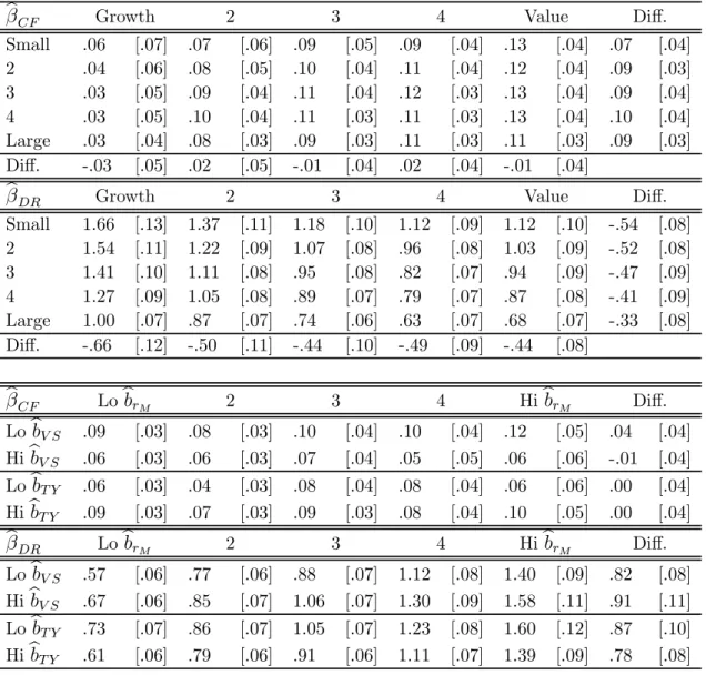
The top half of Table 4 shows the estimated betas for the 25 size and book-to-market portfolios over the period 1929:1—1963:6. The portfolios are organized in a square matrix with growth stocks at the left, value stocks at the right, small stocks at the top, and large stocks at the bottom. At the right edge of the matrix we report the diﬀerences between the extreme growth and extreme value portfolios in each size group; along the bottom of the matrix we report the diﬀerences between the extreme small and extreme large portfolios in each BE/M E category. The top matrix displays cash-flow betas, while the bottom matrix displays discount-rate betas. In square brackets after each beta estimate we report a standard error, calculated conditional on the realizations of the news series from the aggregate VAR model.

In the pre-1963 sample period, value stocks have both higher cash-flow and higher discount-rate betas than growth stocks. An equal-weighted average of the extreme value stocks across size quintiles has a cash-flow beta .16 higher than an equal-weighted average of the extreme growth stocks. The diﬀerence in estimated discount-rate betas is .22 in the same direction. Similar to value stocks, small stocks have higher cash-flow betas and discount-rate betas than large stocks in this sample (by .18 and .36 respectively, for an equal-weighted average of the smallest stocks across value quintiles relative to an equal-weighted average of the largest stocks). In summary, value and small stocks were unambiguously riskier than growth and large stocks over the 1929:1-1963:6 period.

A partial exception to this statement involves the smallest growth portfolio, which is particularly risky and has both cash-flow and discount-rate betas that exceed those of the smallest value portfolio. This small growth portfolio is well known to present a particular challenge to asset pricing models, for example the three-factor model of multiple regression are uncorrelated, and thus the multiple regression coeﬃcients are equal to simple regression coeﬃcients.

(24)

Fama and French (1993) which does not fit this portfolio well. Recent evidence on small growth stocks by Lamont and Thaler (2001), Mitchell, Pulvino, and Staﬀord (2002), D’Avolio (2002) and others suggests that the pricing of some small growth stocks is materially aﬀected by short-sale constraints and other limits to arbitrage. This may help to explain the unusual behavior of the small growth portfolio.

The bottom half of Table 4 shows the cash-flow and discount-rate betas for the risk-sorted portfolios. Both cash-flow betas and discount-rate betas are high for stocks that have had high market betas in the past. Thus, in the early sample period, sorting stocks by their past market betas induces a spread in both cash-flow betas and discount-rate betas. Sorting stocks by their value-spread or term-spread sensitivity induces only a relatively modest spread in either beta.

The patterns are completely different in the post-1963 period shown in Table 5. In this subsample, value stocks still have slightly higher cash-flow betas than growth stocks, but much lower discount-rate betas. The difference in cash-flow betas between the average across extreme value portfolios and the average across extreme growth portfolios is a modest .09. What is remarkable is that the pattern of discount-rate betas reverses in the modern period, so that growth stocks have significantly higher discount-rate betas than value stocks. The difference is economically large (.45) and statistically significant. Recall that cash-flow and discount-rate betas sum up to the CAPM beta; thus growth stocks have higher market betas in the modern period, but their betas are disproportionately of the “good” discount-rate variety rather than the “bad” cash-flow variety.

The changes in the risk characteristics of value and growth stocks that we identify by comparing the periods before and after 1963 are consistent with recent research by Franzoni (2002). Franzoni points out that the market betas of value stocks and small stocks have declined over time relative to the market betas of growth stocks and large stocks. We extend his research by exploring time changes in the two components of market beta, the cash-flow beta and the discount-rate beta.

What economic forces have caused these changes in betas? We suspect that the changing characteristics of value and growth stocks and small and large stocks are related to these patterns in sensitivities. Our first subsample is dominated by the Great Depression and its aftermath. Perhaps in the 1930’s value stocks were fallen angels with a large debt load accumulated during the Great Depression. The higher leverage of value stocks relative to that of growth stocks could explain both the higher cash-flow and expected-return betas of value stocks from 1929—1963. In general, low

(25)

leverage and strong overall position of a company may lead to a low cash-flow beta, and high leverage and weak position to a high cash-flow beta.

We also hypothesize that future investment opportunities, long duration of cash

flows, and dependence on external equity finance lead to a high discount-rate beta. For example, if a distressed firm needed new equity financing simply to survive after the Great Depression, and if the availability and cost of such financing is related to the overall cost of capital, then such afirm’s value is likely to have been very sensitive to discount-rate news. Similarly, new small firms with a negative current cashflow but valuable investment opportunities are likely to be very sensitive to discount-rate news. In the modern subsample, the growth portfolio probably contains a higher proportion of young companies following the initial-public-oﬀering (IPO) wave of the 1960’s, the inclusion of NASDAQfirms in our sample during the late 1970’s, and the

flood of technology IPOs in the 1990’s.

The increase in growth stocks’ discount-rate betas may also be partially explained by changes in stock market listing requirements. During the early period, onlyfirms with significant internal cashflow made it to the Big Board and thus our sample. This is because, in the past, the New York Stock Exchange had very strict profitability requirements for afirm to be listed on the exchange. The low-BE/M E stocks in the

first half of the sample are thus likely be consistently profitable and independent of externalfinancing. In contrast, our post-1963 sample also contains NASDAQ stocks and less-profitable new lists on the NYSE. Thesefirms are listed precisely to improve their access to equity financing, and many of them will not even survive — let alone achieve their growth expectations — without a continuing availability of inexpensive equityfinancing.

Finally, it is possible that our discount-rate news is simply news about investor sentiment. If growth investing has become more popular among irrational investors during our sample period, growth stocks may have become more sensitive to shifts in the sentiment of these investors.

Our risk-sorted portfolios also have diﬀerent betas in the second subsample. Sort-ing on market risk while controllSort-ing for other state variables induces a spread in only the discount-rate beta in the second subsample.

(26)

4

Pricing cash-

fl

We have shown that in the period since 1963, there is a striking diﬀerence in the beta composition of value and growth stocks. The market betas of growth stocks are disproportionately composed of discount-rate betas rather than cash-flow betas. The opposite is true for value stocks.

Motivated by thisfinding, we next examine the validity of a long-horizon investor’s

first-order condition, assuming that the investor holds a 100% allocation to the market portfolio of stocks at all times. We ask whether the investor would be better oﬀ

adding a margin-financed position in some of our test assets (such as value or small stocks), as a short-horizon investor’sfirst-order condition would suggest.

Our main finding is that the long-horizon investor’s first-order condition is not violated by our test assets and that the diﬀerence in beta composition can largely explain the high returns on value and low returns on growth stocks relative to the predictions of the static CAPM. The extreme small-growth portfolio remains an out-lier even in our model, but the returns on this portfolio are not suﬃciently anomalous to cause a statistical rejection of the model.

4.1

An intertemporal asset pricing model

Campbell (1993) derives an approximate discrete-time version of Merton’s (1973) intertemporal CAPM. The model’s central pricing statement is based on the fi rst-order condition for an investor who holds a portfoliopof tradable assets that contains all of her wealth. Campbell assumes that this portfolio is observable in order to derive testable asset-pricing implications from thefirst-order condition.

Campbell considers an infinitely lived investor who has the recursive preferences proposed by Epstein and Zin (1989, 1991):

U(Ct,Et(Ut+1)) = h (1₋δ)C 1−γ θ t +δ ¡ Et ¡ Ut1+1−γ ¢¢1 θi θ 1−γ , (11)

whereCtis consumption at timet,γ >0is the relative risk aversion coeﬃcient,ψ>0

is the elasticity of intertemporal substitution, 0 <δ <1 is the time discount factor, andθ_≡(1₋γ)/(1₋ψ−1). These preferences are a generalization of power utility, for-malized with an objective function (U) that retains the desirable scale-independence

(27)

of the power utility function. Deviating from the power-utility model, however, the Epstein-Zin preferences relax the restriction that the elasticity of intertemporal sub-stitution must equal the reciprocal of the coeﬃcient of relative risk aversion. In the Epstein-Zin model, the elasticity of intertemporal substitution,ψ, and the coeﬃcient of relative risk aversion, γ, are both free parameters.

Campbell assumes that all asset returns are conditionally lognormal, and that the investor’s portfolio returns and its two components are homoskedastic. The assump-tion of lognormality can be relaxed if one is willing to use Taylor approximaassump-tions to the true Euler equations, and the model can be extended to allow changing variances as discussed by Chen (2003). Empirically, changes in volatility seem to be much less persistent than changes in expected returns, and thus they generate relatively modest intertemporal hedging eﬀects on portfolio demands (Chacko and Viceira 1999). For this reason we continue to assume constant variances in the empirical work of this paper.

Campbell derives an approximate solution in which risk premia depend only on the coeﬃcient of relative risk aversion γ and the discount coeﬃcient ρ, and not directly on the elasticity of intertemporal substitution ψ. The approximation is accurate if the elasticity of intertemporal substitution is close to one, and it holds exactly in the limit of continuous time if the elasticity equals one. In theψ= 1case, ρ=δand the optimal consumption-wealth ratio is conveniently constant and equal to1₋ρ. Thus our choice of ρ=.951/12 implies that at the end of each month, the investor chooses to consume .43% of her wealth if ψ= 1.5

Under these assumptions, the optimality of portfolio strategy prequires that the risk premium on any asset isatisfies

Et[ri,t+1]−rf,t+1+

σ2

i,t

2 = γCovt(ri,t+1, rp,t+1−Etrp,t+1) (12) +(1₋γ)Covt(ri,t+1,−Np,DR,t+1),

where p is the optimal portfolio that the agent chooses to hold and Np,DR,t+1 ≡

(Et+1−Et) P∞

j=1ρjrp,t+1+j is discount-rate or expected-return news on this portfolio.

The left hand side of (12) is the expected excess log return on asset i over the riskless interest rate, plus one-half the variance of the excess return to adjust for

5_{Schroder and Skiadas (1999) examine this case in a continuous-time framework which eliminates}

(28)

Jensen’s Inequality. This is the appropriate measure of the risk premium in a log-normal model. The right hand side of (12) is a weighted average of two covariances: the covariance of return i with the return on portfolio p, which gets a weight of γ, and the covariance of return i with negative of news about future expected returns on portfolio p, which gets a weight of (1₋γ). These two covariances represent the myopic and intertemporal hedging components of asset demand, respectively. When γ = 1, it is well known that portfolio choice is myopic and the first-order condition collapses to the familiar one used to derive the pricing implications of the CAPM.

We can rewrite equation (12) to relate the risk premium to covariance with

cash-flow news and discount-rate news. Since rp,t+1−Etrp,t+1 = Np,CF,t+1−Np,DR,t+1,

we have

Et[ri,t+1]−rf,t+1+

σ2

i,t

2 =γCovt(ri,t+1, Np,CF,t+1) + Covt(ri,t+1,−Np,DR,t+1). (13)

Multiplying and dividing by the conditional variance of portfoliop’s return, σ2

p,t, we obtain Et[ri,t+1]−rf,t+1+ σ2 i,t 2 =γσ 2 p,tβi,CFp,t+σ 2 p,tβi,DRp,t. (14)

This equation delivers our prediction that “bad beta” with cash-flow news should have a risk priceγ times greater than the risk price of “good beta” with discount-rate news, which should equal the variance of the return on portfolio p.

In our empirical work, we begin by assuming that portfolio p is fully invested in a value-weighted equity index. This assumption implies that the risk price of discount-rate news should equal the variance of the value-weighted index, about 5% in the early subsample and 2.5% in the modern subsample. The only free parameter in equation (14) is then the coeﬃcient of relative risk aversion,γ.

An alternative assumption would be that portfolio p places a weight w on the value-weighted index and (1−w) on Treasury bills. If the real Treasury-bill return is constant, this would imply that the variance of portfoliopisw2 _{times the variance}

of the index return, while the cash-flow and discount-rate betas of test asset i with portfolio p are (1/w) times the cash-flow and discount-rate betas with the index return. Under this alternative the risk prices for both cash-flow and discount-rate betas are wtimes smaller, but the risk price for the cash-flow beta is stillγ times the risk price for the discount-rate beta. The risk prices of the two betas can be used to identify the two free parameters w andγ.

(29)

4.2

Empirical estimates of risk premia

Would an all-stock investor be better oﬀ holding stocks at market weights or over-weighting value and small stocks? We examine the validity of an unconditional version of thefirst-order condition (14) relative to the market portfolio of stocks. We modify (14) in three ways. First, we use simple expected returns,Et[Ri,t+1−Rrf,t+1],

on the left-hand side, instead of log returns, Et[ri,t+1]−rrf,t+1+σ2i,t/2. In the

log-normal model, both expectations are the same, and by using simple returns we make our results easier to compare with previous empirical studies. Second, we condition down equation (13) to derive an unconditional version of (14) to avoid estimation of all required conditional moments. Finally, we change the subscript p to M and use all-stock investment in the market portfolio of stocks as the reference portfolio, reflecting the fact that we test the optimality of the market portfolio of stocks for the long-horizon investor. These modifications yield:

E[Ri−Rf] =γσ2Mβi,CFM +σ

2

Mβi,DRM (15)

We assume that the log real risk-free rate is approximately constant. We make this assumption mainly because monthly inflation data are unreliable, especially over our long 1928:12-2001:12 sample period. This assumption is unlikely to have a major impact on our tests, since we focus on stock portfolios. The main practical impli-cation of the constant-real-rate assumption is that cash-flow and discount-rate news computed from excess CRSP value-weight index returns are identically equivalent to news terms computed from real CRSP value-weight index returns.

We use 45 test assets, 25 size- and book-to-market sorted portfolios and 20 risk-sorted portfolios, on the left hand side of the unconditionalfirst-order condition (15). We evaluate the performance of the traditional CAPM that restricts cash-flow and discount-rate betas to have the same price of risk, our two-beta intertemporal asset pricing model that restricts the price of discount-rate risk to equal the variance of the market return, and an unrestricted two-beta model that allows free risk prices for cash-flow and discount-rate betas. As discussed above, the unrestricted model can be interpreted as a slight generalization of our model that allows the rational investor’s portfolio to include Treasury bills as well as equities.

Each model is estimated in two diﬀerent forms: one with a restricted zero-beta rate equal to the Treasury-bill rate, and one with an unrestricted zero-beta rate following Black (1972). The first specification includes Treasury bills in the set of

(30)

alternative assets available to the investor, while the second assumes that the investor is considering only reallocations of the portfolio among alternative types of equities. Thus in the first specification we ask the model to explain the unconditional equity premium as well as the premia to value stocks, small stocks, and risk-sorted stocks; in the second specification we remove the equity premium from the set of phenomena to be explained.

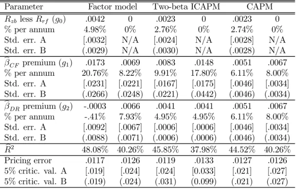
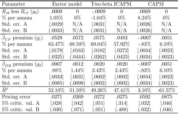
Table 6 reports results for the early sample period 1929:1—1963:6. The table has six columns, two specifications for each of our three asset pricing models. The first nine rows of Table 6 are divided into three sets of four rows. Thefirst set of four rows corresponds to the zero-beta rate (in excess of the Treasury-bill rate), the second set to the premium on cash-flow beta, and the third set to the premium on discount-rate beta. With each set, the first row reports the point estimate in fractions per month, and the second row annualizes this, multiplying by 1200 to ease the interpretation of the estimate. The third and fourth rows present two alternative standard errors of the monthly estimate.

These parameters are estimated from a cross-sectional regression

Re_i =g0+g1βbi,CF +g2bβi,DR+ei, (16)

where bar denotes time-series mean and Re_i _≡ Ri −Rrf denotes the sample average

simple excess return on asseti. The implied risk-aversion coeﬃcient can be recovered as g1/g2.

Standard errors are produced with a bootstrap from 2500 simulated realizations. Our bootstrap experiment samples test-asset returns and VAR errors, and uses the OLS VAR estimates in Table 2 to generate the state-variable data. We partition the VAR errors and test-asset returns into two groups, one for 1929:1-1963:6 and another for 1963:7-2001:12, which enables us to use the same simulated realizations in subperiod analyses. The first set of standard errors (labelled A) conditions on estimated news terms and generates betas and return premia separately for each simulated realization, while the second set (labelled B) also estimates the VAR and the news terms separately for each simulated realization. Standard errors B thus incorporate the considerable additional sampling uncertainty due to the fact that the news terms as well as betas are generated regressors.

Below the premia estimates, we report theRb2 _{statistic for a cross-sectional}

(31)

regressionRb2 _{is computed as} b R2 = 1₋ be 0_b_e ¡ Re_i ₋P_iRe_i¢0¡Re_i ₋P_iRe_i¢ , (17) which allows for negativeRb2 for poorlyfitting models estimated under the constraint that the zero-beta rate equals the risk-free rate.

Although the regression Rb2 _{is intuitive and transparent, it gives equal weight to}

each asset included in the set of test assets even though some assets may be more volatile than others. To address this concern we also report a composite pricing error and its 5% critical value. The composite pricing error is computed ase_b0_Ωb−1_b_{e, where}

b

e is the vector of estimated residuals from regression (16) andΩb is a diagonal matrix with estimated return volatilities on the main diagonal. The weighting matrix,Ωb−1_,

in the composite pricing error formula places less weight on noisy observations yet it is independent of the specific pricing model. We avoid using a freely estimated variance-covariance matrix of test asset returns forΩb because with 45 test assets, we are concerned that the inverse of this matrix would be poorly behaved. Hodrick and Zhang (2001) discuss related alternative methods for assessing the performance of asset pricing models.

Two alternative 5% critical values for the composite pricing error are produced with a bootstrap method similar to the one we have described above, except that the test-asset returns are adjusted to be consistent with the pricing model before the random samples are generated. Critical values A condition on estimated news terms, while critical values B take account of the fact that news terms must be estimated.

Table 6 shows that in the 1929:1—1963:6 period, the traditional CAPM explains the cross-section of stock returns reasonably well, and is comparable to the restricted two-beta model and the two-two-beta model with unrestricted risk prices. The cross-sectional R2 _{statistics are about 40% for models with zero-beta rates equal to the Treasury-bill}

rate, and around 45% for models with unrestricted zero-beta rates. None of the models in the table come close to being rejected at the 5% level.

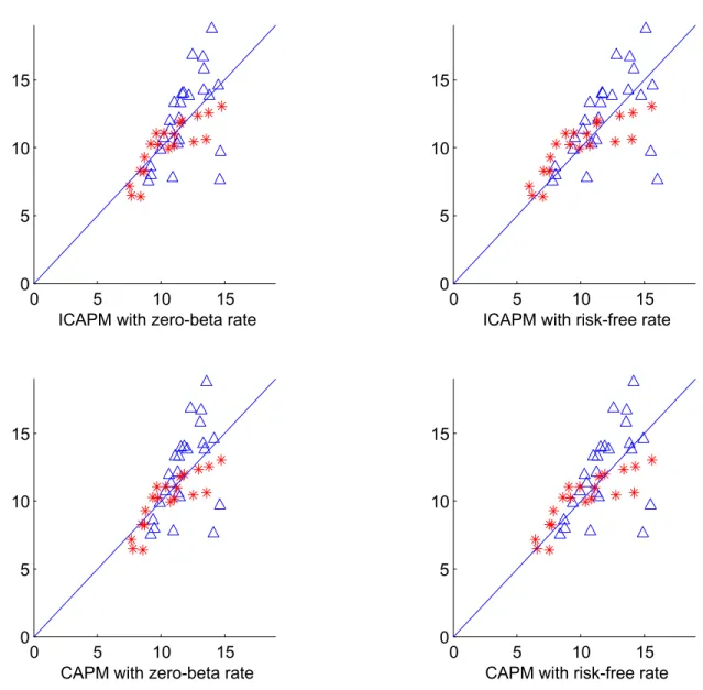
Figure 3 provides a visual summary of these results. Thefigure plots the predicted average excess return on the horizontal axis and the actual sample average excess return on the vertical axis. For a model with a 100% estimated R2_{, all the points}

would fall on the 45-degree line displayed in each graph. The triangles in thefigures denote the 24 Fama-French portfolios and asterisks the 20 risk-sorted portfolios. All

(32)

the models generate nearly identical scatter plots.

The good performance of the CAPM in the 1929—1963 period is due to the fact that in this period, the bad cash-flow beta is roughly a constant fraction of the CAPM beta across assets. Thus our tests cannot discriminate between the static and intertemporal CAPM models in this period.

Results are very diﬀerent in the 1963:7—2001:12 period. Table 7 shows that in this period, the CAPM fails disastrously to explain the returns on the test assets. When the zero-beta rate is left a