The Long-Run Component of Foreign Exchange
Volatility and Stock Returns
Working Paper Series—14-02 | April 2014
Ding Du
Northern Arizona University The W. A. Franke College of Business
PO Box 15066 Flagstaff, AZ 86011.5066 [email protected] (928) 523-7274 Fax: (928) 523-7331
Ou Hu
Department of Economics Youngstown State UniversityYoungstown, OH 44555 [email protected] (330) 941-2061
The Long-Run Component of Foreign Exchange Volatility and
Stock Returns
1. Introduction
The present paper hypothesizes that the long-run component of foreign exchange (FX) volatility is a Merton (1973) state variable in the US equity market. Our conjecture is motivated by the following observations.
First, theoretically models in Campbell (1993, 1996) and Chen (2002) suggest that stock market volatility is a cross-sectional asset-pricing factor with a negative risk premium, because increasing stock market volatility represents a deterioration in investment opportunities. Ang, Hodrick, Xing, and Zhang (2006), Adrian and Rosenberg (2008), Da and Schaumburg (2011), and Moise and Russell (2012) provide supporting evidence. Menkhoff, Sarno, Schmeling, and Schrimpf (2012) (MSSS) concisely conclude that “volatility innovations emerge as a state variable”. (p. 686) 1
Second, there is empirical evidence suggesting that FX volatility spillovers to stock market volatility. For instance, Francis, Hasan, and Hunter (2006) find that increasing FX volatility (except for the Japanese yen) leads to increasing volatility in the US stock market.2 “When (stock) market volatility is stochastic, intertemporal models predict that asset risk premia are not only determined by covariation of returns with the market return, but also by covariation with the state variables that govern (stock) market volatility.” (Adrian and Rosenberg, 2008, p. 2997) In this regard, FX volatility may be a Merton (1973) state variable in the equity market.
Third, two empirical studies imply that it might be the long-run component of FX volatility that matters for asset pricing. First, a recent study by Du and Hu (2012b) shows that FX volatility as a whole has very little pricing power in the US equity market. Second, Bartov, Bodnar, and Kaul (1996) (BBK) find that the market risk of multinational firms increases with the increase in FX volatility when a longer-horizon (5 years) is focused on.3
If only the long-run component of FX volatility matters for the cross-section of stock returns, using raw FX volatility, including both the short- and long-run components, can introduce significant
1 The empirical success of stock market volatility in pricing the cross-section of stock returns has motivated
researchers to use foreign exchange volatility to explain carry trade returns in foreign exchange markets. The empirical evidence in Christiansen, Ranaldo, and Söderlind (2011) and MSSS suggests that foreign exchange volatility is a priced risk factor in the currency market.
2 Muller and Verschoor (2009) also find that “stock return variability of US multinationals is positively
related to exchange rate variability” (p. 1967).
3 Adrian and Rosenberg (2008) also find differential effects of the long-run and short-run components of
noise and reduce the power of tests. Motivated by this observation, we intend to extend Du and Hu (2012b) by focusing on the long-run component of FX volatility in the present paper.
Empirically, we follow MSSS to construct the FX volatility and decompose it into short- and long-run components with the Hodrick and Prescott (1997) methodology. We measure FX volatility innovations in two ways. The first way is to take the first differences of the FX volatility as well as its components as in Ang, Hodrick, Xing, and Zhang (2006), while the second way is to construct factor-mimicking portfolios along the same line as Hou, Karolyi, and Kho (2011). In terms of empirical
implementation, we employ the standard two-pass regression methodology of Fama and MacBeth (1973). Our findings can be easily summarized: the long-run component of FX volatility does have power to explain the cross-section of stock returns. Our findings have important implications for both
international finance and empirical asset pricing. For international finance, we strengthen Francis, Hasan, and Hunter (2006) in that we also suggest researchers focus more on (the long-run component of) the second moment of exchange rates in understanding the linkages between FX and equity markets.4 For empirical asset pricing, we imply a fresh perspective of the state variables underlying the Fama-French-Carhart factors, namely (the long-run component of) FX volatility.
The remainder of the paper is organized as follows: Section 2 describes our data and empirical methodology. Section 3 reports empirical results when FX volatility innovations are measured by the first differences of FX volatility as well as its components. Section 4 presents the results when FX volatility innovations are measured by factor-mimicking portfolio returns. Section 5 concludes the manuscript.
2. Data and empirical methodology
2.1 Data
Following the relevant literature (e.g., MSSS), our full sample includes 34 countries. They are Austria, Australia, Belgium, Brazil, Canada, China, Denmark, Euro Area, Finland, France, Germany, Greece, Hong Kong, India, Ireland, Italy, Japan, Korea, Malaysia, Mexico, Netherlands, New Zealand, Norway, Portugal, Singapore, South Africa, Spain, Sri Lanka, Sweden, Switzerland, Taiwan, Thailand, Venezuela, and United Kingdom. Daily exchange rate data from January 1971 to December 2012 are from the Federal Reserve Bank of St. Louis. The start of the sample period is dictated by the availability of the daily exchange-rate data. Monthly equity-market data are from Kenneth French’s website and the Center for Research in Security Prices (CRSP). 5
4 There is a huge literature that focuses on the first moment of exchange rates. See for instance Adler and
Dumas (1983), Jorion (1990, 1991), Du and Hu (2012a), and Balvers and Klein (2014).
2.2 Empirical methodology
2.2.1 Innovations in FX volatility and its components
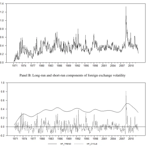
We construct innovations in FX volatility and its components in three steps. First, we follow MSSS to construct the FX volatility. Specifically, (1), we compute the absolute daily log return for each currency on each day in our sample. (2), we average over all currencies available on any given day. (3), we average daily values within any given month to obtain the monthly FX volatility. Panel A of Figure 1 shows the time series of the FX volatility. Several spikes line up with known crises (e.g., the 2008 Financial Crisis).
Figure 1 Foreign exchange volatility 1971:1-2012:12
Panel A: Foreign exchange volatility
Panel B: Long-run and short-run components of foreign exchange volatility
Second, we apply the Hodrick and Prescott (1997) methodology to decompose the FX volatility into the short- and long-run components. The Hodrick and Prescott (1997) methodology is widely used in finance and economics.6 The major advantage of this approach is that it does not require any assumptions about the return-generating process (Cao and Xu, 2010). More specifically, we determine the short- and long-run components of the FX volatility by solving the following programming problem:
, 2 1 1 2 1min
1 trend t trend t trend t trend t T t trend t t fxvfxv
fxv
fxv
fxv
fxv
fxv
T t trend t
(1)where
fxv
tis the FX volatility at timet
, and trend tfxv
is the long-run (trend) component offxv
t. The short-run component of the FX volatility is calculated by subtractingfxv
ttrend fromfxv
t.
is a penalty parameter of the variability in the long-run component of the FX volatility. Hodrick and Prescott (1997) suggest that the value of
should be set equal to 100 times the square of the number of periods in a year. Therefore, for monthly data, we set
equal to 14400. Panel B of Figure 1 shows the short- and long-run components of FX volatility.Third, we construct the innovations of the FX volatility as well as its two components. We construct volatility innovations in two ways. The first way is to take the first differences of the FX volatility and its components as in Ang, Hodrick, Xing, and Zhang (2006).7 The second way is to construct factor-mimicking portfolios along the same line as Fama and French (1993) and Hou, Karolyi, and Kho (2011). The second approach complements the first one. First, changes in the FX volatility and its components are macroeconomic variables (not returns), which may contain information that is irrelevant to asset pricing. In contrast, factor-mimicking portfolios in principle capture only the information in macroeconomic variables that are relevant to stock returns. Therefore, they may help reduce the noise in estimation. Second, to construct factor-mimicking portfolios, we estimate firms’ volatility sensitivities in a rolling regression fashion with 5-year data. Such an approach allows time variation in firm-level volatility sensitivity in a non-structural framework. We choose the 5-year window, because BBK focus on the 5-year horizon.
6 See for instance Adrian and Rosenberg (2008) and Perron and Wada (2009).
7 Using the AR(1) residuals as in MSSS yields qualitatively similar results. However, as MSSS point out,
this approach not only may introduce an errors-in-variables problem but also requires estimation on the full sample which is not implementable (since market participants do not have such information in real time).
2.2.2 Test assets
When innovations in the FX volatility as well as its two components are measured by the first differences, we focus on 25 size and book-to-market (BM) portfolios (which are commonly used in the empirical asset-pricing literature) as our test assets. For robustness, we expand our set of test assets beyond the 25 size and BM portfolios to also include 10 portfolios formed on earnings/price, 10 portfolios formed on cash flow/price, 10 portfolios formed on dividend yield, 10 portfolios formed on short-term reversal, and 10 portfolios formed on long-term reversal. All the monthly portfolio return data are from Kenneth French’s website. The details of the construction of these portfolios are also available at Kenneth French’s website.
When innovations are measured by mimicking portfolio returns, in line with Fama and French (1993) and Hou, Karolyi, and Kho (2011), we construct volatility-sensitivity portfolios as our test assets. The details of the construction of these sensitivity portfolios are discussed in Section 4. For robustness, we also take into account commonly-used stock portfolios formed on size-BM, earnings/price, cash flow/price, dividend yield, short-term reversal, and long-term reversal.
2.2.3 Empirical implementation
To test whether the long-run component of the FX volatility helps explain the cross-section of stock returns, empirically, we focus on the comparison among the following four asset-pricing models. The first model is the Capital Asset Pricing Model of Sharpe (1964) and Lintner (1965) (CAPM):
t i t i MKT i t i
MKT
r
,
,
, (2)where ri,t is the excess return on asset i in period t, and MKTtis the excess market return. The second model is used by Du and Hu (2012b), which enhances the CAPM with the FX volatility (Enhanced CAPM): t i t i VOL t i MKT i t i
MKT
VOL
r
,
,
,
, (3) whereVOL
t is FX volatility innovations. The third model augments the CAPM with the short- and long-run components of the FX volatility (Three-factor model):t i t i LRV t i SRV t i MKT i it
MKT
SRV
LRV
r
,
,
,
, (4)where
SRV
t andLRV
t are innovations of the short- and long-run components of the FX volatility, respectively. The fourth model only takes into account the long-run component of the FX volatility as well as the market factor (Two-factor model):t i t i LRV t i MKT i it
MKT
LRV
r
,
,
, (5)If the long-run component of the FX volatility is priced in the cross-section of stock returns and the short-run component of the FX volatility only introduces noise, we expect that: (1) the Enhanced CAPM would not outperform the CAPM, and the FX volatility would not carry a significant risk
premium; (2) the Three-factor model would outperform the CAPM or the Enhanced CAPM, and the long-run (short-long-run) component of the FX volatility would (not) have a significant risk premium; and (3) the Two-factor model would not underperform the Three-factor model, and the long-run component of the FX volatility would still carry a significant risk premium.
To test our conjectures, we focus on the cross-section of stock returns with the Black, Jensen, and Scholes (1972) and Fama and MacBeth (1973) two-pass regression methodology – estimating factor loadings in the first pass, and using those to obtain risk premiums in the second pass – with standard refinement: the Shanken (1992) correction to obtain errors-in-variables (EIV) robust standard errors, accounting for the fact that factor sensitivities are estimated.
We expect the risk premium on the long-run component of the FX volatility to be negative. The intuition is that a positive innovation in the long-run component of the FX volatility (i.e. unexpected high long-run FX volatility) worsens the investment opportunity set (by increasing stock market volatility). Thus, assets that covary positively with the long-run FX volatility innovations serve as a good hedge against such risk, and should therefore earn a lower expected return. Positive exposure and lower
expected returns of hedging assets imply a negative risk premium on the long-run FX volatility. The same idea implies that if the FX volatility (or its short-run component) is a priced factor, the premium should be negative too (see MSSS).
3 Volatility innovations as first differences
3.1 Main results
Panel A of Table 1 reports the Fama and MacBeth (1973) two-pass OLS regressions with 25 size-BM portfolios as the test assets. Since volatility innovations are measured as the first differences of the FX volatility and its components, our empirical tests cover the sample period from February 1971 to December 2012. The table presents the estimated risk premium associated with each factor with the Shanken (1992) EIV-robust t-statistic in parenthesis. Since we expect the risk premiums on the FX volatility and its components to be negative, the significance of these factors is based on one-sided tests. We also report the OLS cross-sectional adjusted R2.
Table 1 Volatility innovations as first differences
Panel A: Main results
(1) (2) (3) (4) Intercept 1.35 1.45 1.08 1.04 (3.13) (3.82) (2.19) (1.70) MKT -0.63 -0.72 -0.47 -0.44 (-1.33) (-1.69) (-0.86) (-0.68) VOL 2.40 (0.84) SRV 0.54 (0.16) LRV -0.31** -0.32** (-2.18) (-2.01) R2 0.15 0.13 0.30 0.33
Panel B: Robustness checks
GLS 75 test assets (1) (2) (3) (4) (1) (2) (3) (4) Intercept 1.37 1.36 1.37 1.38 0.80 0.84 0.65 0.67 (6.01) (5.85) (5.45) (5.49) (2.53) (2.78) (1.80) (1.72) MKT -0.87 -0.86 -0.86 -0.87 -0.19 -0.23 -0.08 -0.09 (-2.82) (-2.75) (-2.66) (-2.69) (-0.52) (-0.63) (-0.19) (-0.21) VOL -1.66 1.54 (-1.02) (0.78) SRV -1.11 -0.66 (-0.63) (-0.34) LRV -0.15** -0.15** -0.22** -0.22** (-2.34) (-2.44) (-2.00) (-1.89) R2 -1.00 -1.11 -0.62 -0.51 0.01 0.01 0.20 0.21 AR1 innovations 1973:1-2012:12 (1) (2) (3) (4) (1) (2) (3) (4) Intercept 1.35 1.48 1.18 1.14 1.40 1.50 1.25 1.16 (3.13) (4.16) (3.14) (2.20) (3.17) (3.83) (2.60) (2.03) MKT -0.63 -0.75 -0.55 -0.51 -0.67 -0.76 -0.58 -0.49 (-1.33) (-1.84) (-1.25) (-0.92) (-1.37) (-1.70) (-1.07) (-0.80) VOL 2.41 2.50 (0.82) (0.89) SRV 0.42 2.05 (0.14) (0.58) LRV -0.19** -0.19** -0.26** -0.26** (-1.93) (-1.82) (-2.50) (-2.49) R2 0.15 0.13 0.22 0.25 0.15 0.13 0.20 0.22
Table 1 reports the Fama and MacBeth (1973) two-pass regression results. The table presents the estimated risk premium associated with each factor with the Shanken (1992) EIV-robust t-statistic in parenthesis. Since we expect the risk premiums on the FX volatility and its components to be negative, the significance of these factors is based on one-sided tests.
**: significant at the 5% level.
The empirical evidence in Panel A of Table 1 is consistent with our conjecture. First, adding the FX volatility to the CAPM in Column (2) does not improve the model performance: the intercept increases from 1.35 to 1.45 (both are significant at the 5% level), and the cross-sectional R2 decreases
slightly from 0.15 to 0.13. Furthermore, the FX volatility does not carry a statistically significant risk premium. The risk premium of the FX volatility is 2.40 with a t-ratio of 0.84. We therefore are able to reproduce the results of Du and Hu (2012b).
Second, decomposing the FX volatility into its two components helps improve the model performance. Relative to the CAPM in Column (1) or the Enhanced CAPM in Column (2), the Three-factor model in Column (3) has a smaller intercept of 1.08 (although still significant at the 5% level), and a higher cross-sectional R2 of 0.30. More importantly, the long-run component of the FX volatility carries a significantly negative risk premium (its premium is -0.31 with a t-statistic of -2.18), while the short-run component does not (its premium is 0.54 with a t-statistic of 0.16).
Third, including only the long-run component of the FX volatility in Column (4) does not deteriorate the model performance. Compared to the Three-factor model in Column (3), the Two-factor model in Column (4) has a smaller intercept of 1.04 (significant at the 10% level), and a higher cross-sectional R2 of 0.33. Furthermore, the long-run component of the FX volatility still carries a significantly negative risk premium, which is equal to -0.32 with a t-statistic of -2.01. Taken together, all the evidence suggests that it is the long-run component of the FX volatility that has the cross-sectional pricing power. This is the central finding of our paper.
3.2 Robustness checks
We carry out a series of robustness checks. The results are reported in Panel B of Table 1. 3.2.1 GLS regressions
Lewellen, Nagel and Shanken (2010) suggest researchers report not only OLS but also GLS results. We thus report the GLS results in Section “GLS” for 25 size-BM portfolios over the same sample period. Again, the significance of the FX volatility and its components is based on one-sided tests. We also report the GLS cross-sectional adjusted R2. The results are, in principle, consistent with the OLS results in Panel A in that LRV always carries a significantly negative risk premium (while VOL/SRV does not).
3.2.2 Expanded set of test assets
To show that the pricing power of LRV applies to a variety of cross-sections (not just the 25 size-BM portfolios), we expand our set of test assets to 75 portfolios formed on size-size-BM, earnings/price, cash flow/price, dividend yield, short-term reversal, and long-term reversal. Section “75 test assets”
summarizes the cross-sectional regression results. The results are, again, consistent with those in Panel A. (1), LRV always carries a significantly negative risk premium, while VOL/SRV does not. (2), LRV always helps improve the model performance in terms of the intercept and the adjusted R2.
3.2.3 AR(1) residuals as innovations
For robustness, we also follow MSSS by using the AR(1) residuals as innovations. That is, we estimate a simple AR(1) for the FX volatility and use the residuals as our measure for the FX volatility innovation. The same method is applied to the two components of the FX volatility to obtain their innovations. With these new measures, we repeat our tests with 25 size-BM portfolios as our test assets. The results are presented in Section “AR1 innovations”. As we can see, using AR(1) residuals produces qualitatively similar results. First, LRV still carries a significantly negative risk premium, while SRV does not. Second, LRV helps improve the model performance in terms of the intercept and the adjusted R2. 3.2.4 Post-1973 period
An alternative sample period we consider is the post-1973 period (i.e., January 1973 to December 2012). The start of this sample period coincides with the start of fluctuating exchange rates (see BBK). The idea is to see if our results are simply driven by the change in the exchange-rate regime. We repeat our tests with 25 size-BM portfolios as our test assets. The results are presented in Section “1973:1-2012:12”. As we can see, the results are qualitatively similar. (1), LRV still carries a significantly
negative risk premium, while VOL/SRV does not. (2), LRV still helps improve the model performance in terms of the intercept and the adjusted R2.
3.3 Discussion
3.3.1 FX volatility and the Fama-French-Carhart factors
The empirical successes of the Fama-French-Carhart factors (see e.g., Fama and French, 1993; Carhart, 1997) suggest that these factors mimic underlying state variables.8 If the long-run component of FX volatility is a state variable underlying the Fama-French-Carhart factors, we expect that it would lose pricing power when the Fama-French-Carhart factors are present.
We test this conjecture and present the results in Panel A of Table 2. Consistent with our expectation, as soon as the Fama-French-Carhart factors are added, the long-run component of the FX volatility loses its cross-sectional explanatory power. For instance, when the size (SMB), the value (HML), and the momentum (MOM) factors are added, the premium of LRV decreases from -0.31 with a t-statistic of -2.18 (recall Column (3) of Panel A of Table 1) to -0.03 with a t-statistic of -0.39 in Column (3) of Section “Carhart”. Thus, our results complement the empirical asset-pricing literature by suggesting a new state variable underlying the Fama-French-Carhart factors, namely the long-run component of FX volatility.
8 In empirical asset pricing, a voluminous literature has developed to understand what state variables the
Fama-French- Carhart factors may proxy for. See, for instance, Lustig and Van Nieuwerburgh (2004), and Balvers and Huang (2007) among others.
Table 2 Fama-French- Carhart factors and industry portfolios
Panel A: Fama-French-Carhart factors
Fama-French factors Carhart factors
(1) (2) (3) (1) (2) (3) Intercept 1.16 1.28 1.28 0.58 0.63 0.60 (3.82) (4.29) (4.35) (1.35) (1.38) (1.32) MKT -0.65 -0.79 -0.78 -0.04 -0.11 -0.08 (-1.76) (-2.18) (-2.19) (-0.08) (-0.21) (-0.16) SMB 0.13 0.15 0.15 0.14 0.17 0.17 (0.90) (1.04) (1.04) (1.01) (1.23) (1.23) HML 0.41 0.41 0.41 0.41 0.41 0.42 (2.95) (2.93) (2.94) (2.98) (2.95) (2.97) MOM 2.02 2.58 2.62 (2.23) (2.47) (2.49) VOL -1.93 -3.77 (-0.94) (-1.45) SRV -1.94 -3.88 (-0.96) (-1.51) LRV -0.01 -0.03 (-0.14) (-0.39) R2 0.61 0.60 0.58 0.62 0.62 0.61
Panel B: 30 industry portfolios vs. 50 portfolios formed on characteristics
30 industry portfolios 50 portfolios formed on characteristics
(1) (2) (3) (1) (2) (3) Intercept 0.70 0.53 0.48 0.70 -0.07 -0.11 (2.68) (1.83) (1.50) (2.56) (-0.17) (-0.30) MKT -0.12 0.07 0.13 -0.13 0.56 0.61 (-0.34) (0.19) (0.35) (-0.40) (1.29) (1.44) SMB -0.18 -0.14 0.00 0.01 (-0.84) (-0.59) (0.00) (0.05) HML -0.01 0.01 0.40 0.41 (-0.07) (0.04) (2.39) (2.49) MOM 0.30 -0.11 (0.45) (-0.25) R2 -0.01 -0.04 -0.03 0.00 0.61 0.61
Table 2 reports the Fama and MacBeth (1973) two-pass OLS regression results. The table presents the estimated risk premium associated with each factor with the Shanken (1992) EIV-robust t-statistic in parenthesis. We also report the OLS cross-sectional adjusted R2.
3.3.2 Industry portfolios
Lewellen, Nagel and Shanken (2010) suggest that researchers use 30 industry portfolios (in addition to 25 size-BM portfolios) as test assets, because industry portfolios do not have a strong factor structure. However, a lack of factor structure also makes industry portfolios less powerful in
differentiating competing asset-pricing models. We compare three common asset-pricing models in Panel B of Table 2, namely, the CAPM, the Fama-French three-factor model, and the Carhart four-factor model. In Section “30 industry portfolios”, we report the results when 30 industry portfolios are used as test assets. As we can see, none of the Fama-French-Carhart factors is significant, and the cross-sectional R2
ranges from -0.01 to -0.04. Thus, industry portfolios do not have power to differentiate competing asset-pricing models.
The lack of power of industry portfolios motivates us to use portfolios formed on characteristics as additional test assets. In Section “50 portfolios formed on characteristics”, we present the asset-pricing test results for the same three competing models when 50 portfolios formed on earnings/price, cash flow/price, dividend yield, short-term reversal, and long-term reversal are used as test assets. Compared to the CAPM, the Fama-French three-factor model and the Carhart four-factor model significantly improve the model performance. For instance, the cross-sectional R2 increases from 0.00 for the CAPM to 0.61 for the Carhart model, and the intercept decreases correspondingly from 0.70 with a t-statistic of 2.56 to -0.11 with a t-statistic of -0.30. Thus, 50 portfolios formed on characteristics may be more informative in terms of differentiating competing asset-pricing models, and are used as additional test assets in the present paper. 3.3.3 Rolling Hodrick and Prescott (1997) decomposition
So far, we decompose the FX volatility with the full sample. This approach may introduce a possible look-ahead bias. To see if our results are robust to such bias, we implement rolling
decomposition. The decomposition for month t is based on the information available from t – k to t. We update our decomposition monthly by dropping the earliest observation and adding the latest observation. For robustness, we use two windows (i.e., two k values). One is a five years window, and the other is a 10 years window. Panel A of Table 3 reports the results.
In Section “5-year rolling decomposition”, we present the results based on 5-year rolling decomposition. For robustness, we use both 25 size-BM portfolios as well as 75 portfolios (formed on size-BM, earnings/price, cash flow/price, dividend yield, short-term reversal, and long-term reversal) as test assets. As we can see, the results are consistent with those based on full-sample decomposition (in Table 1) in that LRV always carries a significantly negative risk premium (while SRV does not).
The results based on 10-year rolling decomposition in Section “10-year rolling decomposition” are also similar to those based on the full-sample decomposition. Taken together, the evidence suggests that our results are robust to possible look-ahead bias.
3.3.4 Alternative volatility measures
Following MSSS, we compute FX volatility in an equal weighted fashion. For robustness, we try two value-weighted FX volatility measures, and report the results in Panel B of Table 3.
The first value-weighted FX volatility measure is based on the trade weights published by the Board of Governors of the U.S. Federal Reserve System.9 Out of 34 countries in our sample, there are 5
Table 3 Robustness checks
Panel A: Rolling decomposition
5-year rolling decomposition 10-year rolling decomposition
25 size-BM portfolios 75 test assets 25 size-BM portfolios 75 test assets
(1) (2) (1) (2) (1) (2) (1) (2) Intercept 0.84 0.85 0.68 0.68 1.55 1.56 1.03 1.05 (1.38) (1.38) (1.56) (1.61) (2.65) (2.68) (2.62) (2.69) MKT -0.12 -0.13 -0.01 -0.01 -0.87 -0.88 -0.41 -0.43 (-0.18) (-0.19) (-0.01) (-0.02) (-1.35) (-1.37) (-0.90) (-0.95) SRV -4.20* -2.36 -3.11 0.16 (-1.37) (-1.22) (-0.93) (0.08) LRV -1.33** -1.29** -1.00** -1.01** -0.84** -0.78** -0.47** -0.55** (-2.59) (-2.50) (-2.56) (-2.42) (-2.32) (-2.13) (-1.92) (-1.90) R2 0.22 0.25 0.14 0.15 0.38 0.40 0.17 0.17
Panel B: Weighted FX volatility
Trade weights MCI
25 size-BM portfolios 75 test assets 25 size-BM portfolios 75 test assets
(1) (2) (1) (2) (1) (2) (1) (2) Intercept 1.25 1.06 0.82 0.73 1.01 1.17 0.65 0.73 (2.18) (2.12) (2.28) (1.99) (2.10) (2.17) (1.63) (1.79) MKT -0.57 -0.38 -0.22 -0.14 -0.42 -0.58 -0.10 -0.18 (-0.92) (-0.68) (-0.54) (-0.33) (-0.76) (-0.96) (-0.23) (-0.40) SRV 7.50 4.29 -3.02 -2.37** (2.12) (2.08) (-1.18) (-1.96) LRV -0.08* -0.13** -0.05* -0.11** -1.70** -1.78** -1.27* -1.42** (-1.44) (-2.46) (-1.32) (-2.19) (-1.83) (-1.96) (-1.56) (-1.74) R2 0.40 0.19 0.21 0.11 0.23 0.24 0.17 0.15
Table 3 reports the Fama and MacBeth (1973) two-pass regression results. The table presents the estimated risk premium associated with each factor with the Shanken (1992) EIV-robust t-statistic in parenthesis. We also report the cross-sectional adjusted R2.
**: significant at the 5% level. *: significant at the 10% level.
countries that do not have trade weights - Denmark, Norway, South Africa, Sri Lanka, and New Zealand. Therefore, the value-weighted FX volatility is based on 29 currencies. Essentially, (1) we compute the FX volatility in the same way as in Section 2.2 except that we average individual currency volatility in a value-weighed fashion based on their trade weights; (2) we decompose the FX volatility by using the Hodrick and Prescott (1997) methodology; (3) we repeat our asset-pricing tests and report the results in Section “Trade weights”. For robustness, again, we use both 25 size-BM portfolios as well as 75 portfolios (formed on size-BM, earnings/price, cash flow/price, dividend yield, short-term reversal, and long-term reversal) as test assets. As we can see, the results are consistent with those based on the equal-weighted FX volatility (in Table 1) in that LRV always carries a significantly negative risk premium (while SRV does not).
The second value-weighted FX volatility measure is based on the Major Currencies Index (MCI) from the Board of Governors, which is a trade-weighted currency index.10 Following Adrian and
Rosenberg (2008), we first estimate a GARCH (1, 1) model on the daily MCI to obtain the daily MCI volatility. Next, using the Hodrick and Prescott (1997) approach, we decompose the daily MCI volatility into a long-run component and a short-run component. After fitting an AR(1) model on each component, we compute the daily innovations of the volatility components by subtracting the values expected 21 days earlier from their observed values. Finally, we sum these innovations over the days in each month to obtain the monthly innovations of the short- and long-run components of the FX volatility.The results are reported in Section “MCI”. Our sample period is from January 1973 to December 2012. The start of the sample is dictated by the availability of the MCI data. Again, the results are similar to those based on the equal-weighted FX volatility (in Table 1): LRV always carries a significantly negative risk premium, while SRV does not.
4. Volatility innovations as factor-mimicking portfolio returns
4.1 Volatility mimicking portfolios
Along the same line as Fama and French (1993) and Hou, Karolyi, and Kho (2011), we construct our FX-volatility factor-mimicking portfolios. For the ease of exposition, our description focuses on the construction of the VOL factor-mimicking portfolio. The same procedure applies to the construction of the factor-mimicking portfolios for SRV and LRV.
We construct the VOL factor-mimicking portfolio in two steps. The first step is to form 25 value-weighted VOL-sensitivity portfolios with all the stocks in CRSP. The portfolios are constructed at the end of each June based on firm-level VOL-sensitivity, which is estimated with the prior five years’ data. As a result, our test period in this section is from 1978:7 to 2010:12. Again, the 5-year window is chosen due to BBK. Firm-level VOL-sensitivity is estimated with Eq. (3) (i.e., the Enhanced CAPM). These
portfolios are held for one year from July of year t to June of year t+1 and rebalanced at the end of June of year t+1. By rebalancing the portfolios on an annual basis in a conditional fashion, we allow firms’ VOL sensitivity to be time varying.
The second step is to define the factor-mimicking portfolio return as the average return on the five positive VOL-sensitivity portfolios minus the average return on the five negative VOL-sensitivity portfolios. The idea of using five positive/negative VOL-sensitivity portfolios is to avoid mimicking
10 MCI is a weighted average of the foreign exchange values of the U.S. dollar against currencies of major
industrial countries. The Major Currency Index includes the Euro Area, Canada, Japan, United Kingdom, Switzerland, Australia, and Sweden.
portfolio returns being driven by extreme portfolio returns (see Hou, Karolyi, and Kho, 2011). We use the same procedure to construct the mimicking portfolios for SRV and LRV, except that firm-level SRV-sensitivity and LRV-SRV-sensitivity are estimated with Eq. (4) (i.e., the Three-factor model).
If LRV is a priced factor and carries a negative risk premium, we would expect that the portfolios with positive sensitivity to LRV serve as a hedge against such risk and earn lower mean/expected returns, and the portfolios with negative sensitivity to LRV expose to such risk and earn higher mean/expected returns. The evidence in Table 4 is consistent with our expectation. Table 4 shows the mean returns and other relevant summary statistics of the 25 LRV-sensitivity portfolios. These 25 portfolios are ranked by their sensitivity to LRV. For instance, Portfolios 1 to 5 consist of the US stocks with the most negative sensitivity to LRV, while Portfolios 21 to 25 include those stocks with the most positive sensitivity to LRV. As we can see, the mean return of these LRV-sensitivity portfolios, as we expect, generally decreases monotonically with the LRV-sensitivity. As a result, the mean return of the LRV mimicking portfolio (which is equal to the average return of Portfolios 21 to 25 minus that of Portfolios 1 to 5) is significantly negative (it is -0.37% per month with a t-statistic of -1.81, which is significant at the 5% level for a one-sided test).11
If SRV is not a priced factor, we would not expect the same pattern in the cross-section of the SRV-sensitivity portfolios. The evidence in Table 5 is consistent with this expectation. Table 5 shows the mean returns and other relevant summary statistics of the 25 SRV-sensitivity portfolios. These 25
portfolios are ranked by their sensitivity to SRV. As we can see, the mean return of these SRV-sensitivity portfolios does not decrease monotonically with the SRV-sensitivity. As a result, the mean return of the SRV mimicking portfolios (which is equal to the average return of Portfolios 21 to 25 minus that of Portfolios 1 to 5) is insignificantly different from zero (it is 0.10% per month with a t-statistic of 0.65).
Table 4 Mean Returns of 25 Long-run Sensitivity Portfolios Portfolio Number of firm months Sensitivity Size Average monthly raw return Estimate Percent Positive Percent significant at 10% level P1 36061 -1.45 0.00 0.59 1297643 1.36 P2 36907 -0.94 0.00 0.26 1654791 1.28 P3 37057 -0.74 0.00 0.16 2433027 1.40 P4 37382 -0.61 0.00 0.09 2443112 1.42 P5 37422 -0.52 0.00 0.06 2710481 1.09 P6 37456 -0.44 0.00 0.04 2761092 1.28 P7 37908 -0.37 0.00 0.02 3043586 1.10 P8 37837 -0.31 0.02 0.03 2525256 1.36 P9 37891 -0.26 0.12 0.02 2821277 0.89 P10 37948 -0.21 0.15 0.01 2695769 1.09 P11 38117 -0.16 0.35 0.01 2579791 1.02 P12 38000 -0.12 0.45 0.01 2500509 1.15 P13 37924 -0.07 0.51 0.01 2441369 1.06 P14 38048 -0.03 0.60 0.01 2616981 1.10 P15 38080 0.01 0.70 0.01 2932805 1.18 P16 37929 0.05 0.76 0.01 2522435 0.96 P17 38039 0.10 0.81 0.01 2562412 1.29 P18 37870 0.14 0.83 0.01 2539471 1.10 P19 38092 0.19 0.90 0.02 2365363 1.14 P20 37799 0.25 0.93 0.03 2841969 1.10 P21 37603 0.32 0.97 0.05 2504275 0.89 P22 37519 0.41 1.00 0.09 2662222 0.92 P23 37233 0.53 1.00 0.15 2430035 0.86 P24 37190 0.70 1.00 0.24 2425344 0.92 P25 41009 1.20 1.00 0.53 2363783 1.11
5 1 25 21 5 1 i i i i P P -0.37** (-1.81) We form 25 value-weighted LRV-sensitivity portfolios with all the stocks in CRSP. Table 4 shows the mean returns and other relevant summary statistics of these sensitivity portfolios. These 25 portfolios are ranked by their sensitivity to LRV. For instance, Portfolios 1 to 5 consist of the US stocks with the most negative sensitivity to LRV, while Portfolios 21 to 25 include those stocks with the most positive sensitivity to LRV. LRV-sensitivity is estimated over a five-year period. Size is calculated as the price times the number of shares outstanding in June of year t. The table shows portfolio averages for size, LRV-sensitivity, and returns. Firm months used in each portfolio are shown too, along with the percentage of firm months for which LRV-sensitivity is positive or significant at the 10% level over the formation period.Table 5 Mean Returns of 25 short-run Sensitivity Portfolios Portfolio Number of firm months Sensitivity Size Average monthly raw return Estimate Percent Positive Percent significant at 10% level P1 36873 -0.33 0.00 0.61 1413030 1.24 P2 37287 -0.21 0.00 0.30 2028838 1.05 P3 37159 -0.16 0.00 0.15 2205497 1.11 P4 37558 -0.13 0.00 0.07 2756941 1.32 P5 37451 -0.11 0.00 0.04 2558719 1.04 P6 37621 -0.09 0.00 0.02 2877549 1.11 P7 37668 -0.07 0.00 0.01 3124935 1.08 P8 37676 -0.06 0.00 0.01 2847024 0.74 P9 37850 -0.05 0.00 0.00 2315194 1.10 P10 37830 -0.03 0.06 0.01 2675629 1.02 P11 37677 -0.02 0.19 0.00 2857278 1.08 P12 37753 -0.01 0.44 0.00 2558498 1.12 P13 37985 0.00 0.57 0.00 2513626 1.13 P14 37964 0.01 0.73 0.00 2657053 1.04 P15 37983 0.02 0.81 0.00 2334656 1.08 P16 37976 0.03 0.91 0.01 2454860 1.12 P17 37745 0.04 0.92 0.02 2717253 1.13 P18 37727 0.05 0.94 0.02 2774725 1.28 P19 38069 0.07 0.97 0.04 2732126 1.10 P20 37603 0.08 1.00 0.05 2294570 1.27 P21 37520 0.10 1.00 0.07 2671609 1.18 P22 37435 0.12 1.00 0.12 2922741 1.29 P23 37520 0.15 1.00 0.20 2612342 1.29 P24 37314 0.19 1.00 0.33 2461951 1.07 P25 41077 0.31 1.00 0.58 1390520 1.44
5 1 25 21 5 1 i i i i P P 0.10 (0.65) We form 25 value-weighted SRV-sensitivity portfolios with all the stocks in CRSP. Table 5 shows the mean returns and other relevant summary statistics of these sensitivity portfolios. These 25 portfolios are ranked by their sensitivity to SRV. For instance, Portfolios 1 to 5 consist of the US stocks with the most negative sensitivity to SRV, while Portfolios 21 to 25 include those stocks with the most positive sensitivity to SRV. SRV-sensitivity is estimated over a five-year period. Size is calculated as the price times the number of shares outstanding in June of year t. The table shows portfolio averages for size, SRV-sensitivity, and returns. Firm months used in each portfolio are shown too, along with the percentage of firm months for which SRV-sensitivity is positive or significant at the 10% level over the formation period.Because VOL contains SRV, it may be too noisy to be a priced factor. Thus, we would not expect any pattern in the cross-section of the VOL-sensitivity portfolios. The evidence in Table 6 is consistent with this expectation. As we can see, the mean return of the VOL mimicking portfolios (which is equal to the average return of Portfolios 21 to 25 minus that of Portfolios 1 to 5) is insignificantly different from zero (it is -0.00% per month with a t-statistic of -0.01).
Table 6 Mean Returns of 25 VOL-sensitivity Portfolios Portfolio Number of firm months Sensitivity Size Average monthly raw return Estimate Percent Positive Percent significant at 10% level P1 36643 -0.30 0.00 0.61 1268756 1.26 P2 37031 -0.20 0.00 0.34 1977817 1.22 P3 37388 -0.15 0.00 0.18 2357484 0.96 P4 37397 -0.13 0.00 0.08 2378613 1.14 P5 37542 -0.11 0.00 0.05 2631065 1.14 P6 37465 -0.09 0.00 0.03 2864702 1.04 P7 37659 -0.07 0.00 0.02 2548448 1.18 P8 37762 -0.06 0.00 0.01 2912648 1.04 P9 37766 -0.05 0.00 0.00 3144365 1.06 P10 37717 -0.04 0.10 0.00 2420934 1.06 P11 37895 -0.03 0.28 0.00 2454114 1.17 P12 38168 -0.02 0.37 0.00 2390177 1.14 P13 37784 -0.01 0.45 0.00 2428732 1.15 P14 37785 0.00 0.59 0.00 2541400 0.98 P15 37895 0.01 0.71 0.00 2343660 1.07 P16 37824 0.02 0.80 0.00 2415582 0.99 P17 37923 0.03 0.90 0.01 2575014 1.19 P18 37772 0.04 0.97 0.01 2522565 1.23 P19 37721 0.05 0.98 0.02 2218920 1.30 P20 37791 0.07 1.00 0.05 2547080 1.30 P21 37744 0.08 1.00 0.09 2663204 0.99 P22 37607 0.10 1.00 0.15 2790863 1.16 P23 37409 0.13 1.00 0.23 3070772 1.25 P24 37187 0.16 1.00 0.33 2969429 1.19 P25 41446 0.27 1.00 0.58 2234388 1.12
5 1 25 21 5 1 i i i i P P -0.00 (-0.01) We form 25 value-weighted VOL-sensitivity portfolios with all the stocks in CRSP. Table 6 shows the mean returns and other relevant summary statistics of these sensitivity portfolios. These 25 portfolios are ranked by their sensitivity to VOL. For instance, Portfolios 1 to 5 consist of the US stocks with the most negative sensitivity to VOL, while Portfolios 21 to 25 include those stocks with the most positive sensitivity to VOL. VOL-sensitivity is estimated over a five-year period. Size is calculated as the price times the number of shares outstanding in June of year t. The table shows portfolio averages for size, VOL-sensitivity, and returns. Firm months used in each portfolio are shown too, along with the percentage of firm months for which VOL-sensitivity is positive or significant at the 10% level over the formation period.The evidence in Tables 5 and 6 (as well as that in Tables 1 and 3) suggests that VOL and SRV are not priced in the US equity market. Therefore, in this section, we focus on the comparison between CAPM and the Two-factor model (which enhances the CAPM with LRV). The idea is to demonstrate the performance improvement that LRV can bring about.
Following the empirical asset-pricing literature, we use the LRV-sensitivity portfolios in Table 4 as our test assets. For robustness, we also take into account commonly-used stock portfolios formed on size-BM, earnings/price, cash flow/price, dividend yield, short-term reversal, and long-term reversal.
Table 7 Volatility innovations as factor-mimicking portfolio returns Panel A: 25 LRV-sensitivity portfolios
(1) (2) Intercept 0.76 0.29 (1.93) (0.74) MKT -0.09 0.37 (-0.20) (0.80) LRV -0.35** (-2.03) R2 -0.04 0.51
Panel B: Robustness checks GLS
25 size-sensitivity
portfolios 75 test assets 125 test assets
(1) (2) (1) (2) (1) (2) (1) (2) Intercept 0.46 0.26 1.03 0.89 0.94 0.45 1.03 0.78 (1.32) 0.70) (5.02) (4.49) (2.54) (0.98) (4.35) (3.41) MKT 0.19 0.40 -0.23 -0.13 -0.25 0.14 -0.33 -0.12 (0.44) (0.89) (-0.77) (-0.43) (-0.58) (0.28) (-1.00) (-0.37) LRV -0.37* -0.43** -0.95** -0.48** (-1.47) (-2.26) (-2.24) (-2.53) R2 -0.14 0.51 0.03 0.32 0.04 0.41 0.08 0.34
Table 7 reports the Fama and MacBeth (1973) two-pass regression results. The table presents the estimated risk premium associated with each factor with the Shanken (1992) EIV-robust t-statistic in parenthesis. Since we expect the risk premiums on the long-run component of the FX volatility to be negative, the significance of this factors is based on one-sided tests.
**: significant at the 5% level. *: significant at the 10% level.
4.2 Main results
Panel A of Table 7 summarizes the results of the OLS Fama-MacBeth regressions when the 25 LRV-sensitivity portfolios are used as` test assets. The table presents the estimated risk premium
associated with each factor with the Shanken (1992) EIV-robust t-statistic in parenthesis. Since we expect that the risk premium on LRV would be negative, the significance of LRV is based on one-sided tests.
As we can see, using the mimicking-portfolio approach yields consistent results. First, the LRV mimicking portfolio carries a significantly negative risk premium. The risk premium is -0.35% per month with a t-statistic of -2.03. Second, the Two-factor model that enhances the CAPM with LRV outperforms the CAPM significantly. The intercept of the Two-factor model is 0.29 (t-statistic= 0.74), while that of the CAPM is 0.76 (t-statistic = 1.93). The adjusted R2 of the Two-factor model is 0.51, while that of the CAPM is -0.04.
4.3 Robustness checks
We carry out a series of robustness checks. The results are reported in Panel B of Table 7. 4.3.1 GLS regressions
We report the GLS results in Section “GLS” for 25 LRV-sensitivity portfolios over the same sample period. The results are, in principle, consistent with the OLS results in Panel A. First, LRV carries a significantly negative risk premium. Second, LRV helps improve the model performance in terms of the adjusted R2.
4.3.2 Alternative test assets
To show that the pricing power of LRV applies to a variety of cross-sections (not just the 25 LRV-sensitivity portfolios), we try two alternative sets of test assets. The first set is the 25 size-and-LRV sensitivity portfolios. The idea is to take into account the size effect well-documented in the empirical asset-pricing literature. Essentially, we form 25 value-weighted size-and-LRV sensitivity portfolios with all the stocks in CRSP. The portfolios, which are constructed at the end of each June, are the intersections of five portfolios formed on size (market capitalization) and five portfolios formed on LRV sensitivity. Again, the LRV sensitivity for June of year t is estimated with the prior five years’ data based on the Eq. (4). These portfolios are held for one year from July of year t to June of year t+1 and rebalanced at the end of June of year t+1.
The second set of test assets consists of 75 commonly-used stock portfolios formed on size-BM, earnings/price, cash flow/price, dividend yield, short-term reversal, and long-term reversal. Sections “25 size-sensitivity portfolios” and “75 test assets” summarize the cross-sectional regression results. The results are, again, consistent with those in Panel A. (1), LRV always carries a significantly negative risk premium. (2), LRV always helps improve the model performance in terms of the intercept and the adjusted R2.
4.3.3 Expanded set of test assets
To get an idea of the overall pricing power of LRV, we repeat the tests with all 125 test assets we have used. They are 75 commonly-used stock portfolios (formed on size-BM, earnings/price, cash
flow/price, dividend yield, short-term reversal, and long-term reversal), 25 LRV-sensitivity portfolios, and 25 size and LRV-sensitivity portfolios. Section “125 test assets” presents the cross-sectional regression results. For a wide variety of test assets, LRV carries a significantly negative risk premium of -0.48% per month (with a t-statistic of -2.53). Furthermore, LRV helps reduce the intercept from 1.03 (t-statistic=4.35) to 0.78 (t-statistic=3.41), and increase the adjusted-R2 from 0.08 to 0.34. Thus, all the evidence suggests that the long-run component of FX volatility is a statistically significant Merton (1973) factor.
4.4 Economic significance of FX volatility
To shed light on the economic significance of the long-run component of the FX volatility, we calculate the mean excess return explained by LRV, which is the product of the average absolute LRVexposure
Table 8 Time series regressions Portfolio Alpha MKT LRV R2 P1 -0.01 1.22 -0.59 0.74 ( -0.07 ) ( 14.58 ) ( -6.09 ) P2 -0.00 1.10 -0.54 0.83 ( -0.01 ) ( 33.09 ) ( -11.19 ) P3 0.18 0.96 -0.59 0.77 ( 1.27 ) ( 19.70 ) ( -10.23 ) P4 0.13 1.06 -0.61 0.82 ( 1.34 ) ( 18.37 ) ( -10.12 ) P5 -0.08 0.94 -0.48 0.81 ( -0.72 ) ( 17.98 ) ( -8.41 ) P6 0.17 0.92 -0.33 0.78 ( 2.04 ) ( 21.69 ) ( -6.19 ) P7 0.08 0.90 -0.13 0.72 ( 0.73 ) ( 21.82 ) ( -1.55 ) P8 0.26 0.92 -0.32 0.73 ( 2.40 ) ( 18.61 ) ( -4.03 ) P9 -0.15 0.90 -0.21 0.72 ( -1.11 ) ( 19.36 ) ( -3.18 ) P10 0.03 0.88 -0.26 0.78 ( 0.32 ) ( 26.54 ) ( -6.07 ) P11 0.01 0.95 -0.03 0.71 ( 0.09 ) ( 28.25 ) ( -0.29 ) P12 0.15 0.90 -0.10 0.71 ( 1.36 ) ( 25.79 ) ( -1.09 ) P13 0.09 0.81 -0.14 0.70 ( 0.75 ) ( 18.58 ) ( -1.87 ) P14 0.09 0.86 -0.18 0.77 ( 0.75 ) ( 20.85 ) ( -2.65 ) P15 0.19 0.83 -0.16 0.70 ( 1.75 ) ( 18.43 ) ( -1.71 ) P16 -0.03 0.89 -0.08 0.76 ( -0.25 ) ( 26.31 ) ( -1.59 ) P17 0.33 0.89 -0.01 0.76 ( 2.92 ) ( 20.00 ) ( -0.16 ) P18 0.14 0.86 -0.05 0.80 ( 1.17 ) ( 28.21 ) ( -0.76 ) P19 0.19 0.89 0.04 0.77 ( 2.04 ) ( 26.72 ) ( 0.54 ) P20 0.22 0.91 0.24 0.78 ( 1.80 ) ( 29.00 ) ( 5.06 ) P21 -0.01 0.97 0.32 0.81 ( -0.05 ) ( 21.77 ) ( 4.86 ) P22 0.03 0.96 0.29 0.82 ( 0.24 ) ( 22.66 ) ( 3.69 ) P23 -0.00 1.02 0.46 0.86 ( -0.01 ) ( 36.55 ) ( 6.17 ) P24 0.03 1.09 0.50 0.83 ( 0.18 ) ( 39.76 ) ( 7.83 ) P25 0.17 1.25 0.61 0.83 ( 1.05 ) ( 28.91 ) ( 7.05 )
The time-series regression results are reported in Table 8. The t-ratios are based on Newey-West HAC standard errors with the lag parameter set equal to 12. The test assets are 25 LRV-sensitivity portfolios
exposure (from first-pass time-series regressions) and the absolute LRV risk premium (from the second-pass cross-sectional regression).
The time-series regression results are reported in Table 8. The t-ratios are based on Newey-West HAC standard errors with the lag parameter set equal to 12. The test assets are 25 LRV-sensitivity
portfolios. 18 out of 25 (or 72%) of our test assets have significant exposure to the long-run component of the FX volatility (at the 10% level). The average absolute LRV exposure is 0.29. Panel A of Table 7 shows that, for the same test assets, the risk premium on LRV is -0.35 percent per month (which is very close to the premium estimates in Tables 1 and 4). Taken together, the mean excess return explained by LRV is 0.29 × 0.35 = 0.10 percent per month (or 1.23 percent per year). Since the average excess return on 25 LRV-sensitivity portfolios is 0.67 percent per month (8.38 percent per year), LRV explains about 15 percent of the mean excess return of our test assets, which seems to be economically significant.
5. Conclusion
The present paper hypothesizes that the long-run component of foreign exchange volatility is a Merton (1973) state variable in the US equity market. We find robust evidence supporting our conjecture. Our findings have important implications for both international finance and empirical asset pricing. For international finance, we strengthen Francis, Hasan, and Hunter (2006) in that we suggest researchers focus more on the second moment of exchange rates in understanding the relationship between currency and equity markets. For empirical asset pricing, we imply a fresh perspective of the state variables underlying the Fama-French-Carhart factors, namely the long-run component of foreign-exchange volatility.
References
Adler, M., and Dumas, B., 1983. International portfolio choice and corporate finance: a synthesis. Journal of Finance, 38, 925-984.
Adrian, Tobias, and Joshua Rosenberg, 2008. Stock returns and volatility: Pricing the short-run and long-run components of market risk, Journal of Finance, 63, 2997-3030.
Ang, Andrew, Robert Hodrick, Yuhang Xing, and Xiaoyan Zhang, 2006. The cross-section of volatility and expected returns, Journal of Finance, 61, 259-299.
Balvers, R., and D. Huang, 2007. Productivity-Based Asset Pricing: Theory and Evidence, Journal of Financial Economics, 86, 405-445.
Balvers, R., and A. F. Klein, 2014. Currency risk premia and uncovered interest parity in the international CAPM, Journal of International Money and Finance, 41, 214-230.
Bartov, E., Bodnar, Gordon M., and Kaul, Aditya, 1996. Exchange rate variability and the riskiness of U.S. multinational firms: Evidence from the breakdown of the Bretton Woods system, Journal of Financial Economics, 42, 105-132.
Black, F., M. C. Jensen, and M. Scholes, 1972. The Capital Asset Pricing Model: Some Empirical Findings; in Michael C. Jensen, ed.: (Praeger, New York). Studies in the Theory of Capital Markets Campbell, John Y., 1993. Intertemporal asset pricing without consumption data, American Economic
Review, 83, 487–512.
Campbell, John Y., 1996. Understanding risk and return, Journal of Political Economy, 104, 298–345. Cao, Xuying, and Yexiao Xu, 2010. Long-run Idiosyncratic Volatilities and Cross-sectional stock returns,
Working paper, University of Texas at Dallas.
Carhart, M. M. 1997. On Persistence in Mutual Fund Performance. Journal of Finance 52, 57–82. Chen, Joseph, 2002. Intertemporal, CAPM and the cross-section of stock returns, Working paper,
University of Southern California.
Christiansen, Charlotte, Angelo Ranaldo, and Paul Söderlind, 2011. The time-varying systematic risk of carry trade strategies, Journal of Financial and Quantitative Analysis, 46, 1107–1125.
Da, Zhi, and Ernst Schaumburg, 2011. The pricing of volatility risk across asset classes and the Fama-French factors, Working paper, Northwestern University.
Du, D., and Hu, O. 2012a. Exchange rate risk in the US stock market. Journal of International Financial Markets, Institutions & Money 22, 137– 150.
Du, D. & Hu, O. 2012b. Foreign Exchange Volatility and Stock Returns. Journal of International Financial Markets, Institutions & Money, 22, 1202– 1216.
Fama, E. F., French, K. R., 1993. Common risk factors in the returns on stocks and bonds. Journal of Financial Economics, 33, 3–56.
Fama, E. F., and J. D. MacBeth, 1973. Risk, Return and Equilibrium: Empirical Tests, Journal of Political Economy 81, 607-636.
Francis, B., I Hasan, and D. Hunter, .2006. Dynamic Relations between International Equity and Currency Markets: The Role of Currency Order Flow, Journal of Business, 79, 219-258. Hodrick, R. J., and E. C. Prescott, 1997. Postwar U.S. business cycles: An empirical investigation,
Journal of Money, Credit, and Banking 29, 1–16.
Hou, K., A. Karolyi and B. Kho, 2011, What Factors Drive Global Stock Returns?,Review of Financial Studies, 24, 2527-2574.
Jorion, P., 1990. The exchange-rate exposure of U.S. multinationals. Journal of Business, 63, 331-345 Jorion, P. 1991. The Pricing of Exchange Rate Risk in the Stock Market, Journal of Financial and
Quantitative Analysis, 26:3: 363-376.
Lewellen, J. W., Nagel, S., and Shanken, J. A., 2010. A Skeptical Appraisal of Asset Pricing Tests,
Journal of Financial Economics 96, 175-194.
Lintner, John, 1965. The valuation of risk assets and the selection of risky investments in stock portfolios and capital budgets, Review of Economics and Statistics, 47, 13-37.
Lustig, Hanno and Stijn Van Nieuwerburgh, 2004. Housing collateral, consumption insurance, and risk premia. Journal of Finance, 60, 1167-1221.
Menkhoff, Lukas & Sarno, Lucio & Schmeling, Maik & Schrimpf, Andreas, 2012. Carry Trades and Global Foreign Exchange Volatility, Journal of Finance, 67, 681-718.
Merton, R. C., 1973. An intertemporal capital asset pricing model, Econometrica, 41, 867-887. Moise, Claudia E. and Jeffrey R. Russell, 2012. The joint pricing of volatility and liquidity, Working
paper, University of Chicago.
Muller, Aline, Willem F.C. Verschoor. 2009. The effect of exchange rate variability on US shareholder wealth, Journal of Banking & Finance, 33, 1963-1972,
Perron, Pierre; Wada, Tatsuma, 2009, Let's Take a Break: Trends and Cycles in US Real GDP, Journal of Monetary Economics, 56, 749-765.
Shanken, J., 1992, On the Estimation of Beta-Pricing Models, Review of Financial Studies 5, 1-33. Sharpe, William F., 1964, Capital asset prices: A theory of market equilibrium under conditions of risk,