The Effects of Credit Subsidies on Development
∗
Ant´
onio Antunes
†Tiago Cavalcanti
‡Anne Villamil
§March 5, 2014
Abstract
Under credit market imperfections, the marginal product of capital may not be equalized, resulting in misallocation and lower output. Preferential interest rate policies are often used to remedy the problem. This paper con-structs a general equilibrium model with heterogeneous agents, imperfect en-forcement and costly intermediation. Occupational choice and firm size are determined endogenously by an agent’s type (ability and net wealth) and credit market frictions. The credit program subsidizes the interest rate on loans and requires a fixed application cost, which might be null. We find that the credit subsidy policy has no significant effect on output, but it may have negative effects on wages. The program is largely a transfer from households to a small group of entrepreneurs with minor aggregate effects. We also provide estimates of the effects of reducing the frictions directly. When comparing differences in U.S. output per capita in a baseline case to simulations with counterfactually high frictions, intermediation costs and enforcement explain about 20-25% of the output gap. We include a transition analysis.
Keywords: Financial frictions; Credit subsidy; Entrepreneurship JEL Classification: E60; G38; O11
∗We thank Breno Albuquerque, Francesco Caselli, M´ario Centeno, Fernando de Holanda Bar-bosa Filho, Giammario Impullitti, Marcelo Mello, Marcelo dos Santos, Andr´e Silva, Arilton Tei-xeira, and Pedro Teles for helpful comments and suggestions. We have also benefited from com-ments by audiences at the EPGE/CAEN Meeting, Lisbon Meeting on Institutions and Political Economy, LuBraMacro meeting, REAP Meeting, Rice University, SAET Meeting, INSPER-SP, PIMES/UFPE, PUC-RJ, Thema-Cergy, University of Cambridge, University of Illinois, and the Workshop on Advances in Economic Growth at University of St. Andrews. We thank for financial support INOVA and Funda¸c˜ao para a Ciˆencia e Tecnologia, grant PTDC/EGE-ECO/108858/2008, and Keynes Fund from the University of Cambridge.
†Departamento de Estudos Econ´omicos, Banco de Portugal. Email: antunesaa@gmail.com. ‡Faculty of Economics, University of Cambridge. Email: tvdvc2@cam.ac.uk.
§Department of Economics, University of Iowa and University of Manchester.
1
Introduction
When markets function perfectly inequality reflects differences in effort, innate abil-ity to acquire skills, manage a labor force, or deploy capital. Even when initial wealth is unequal, more talented entrepreneurs with low initial wealth will borrow to acquire capital (if entrepreneurial talent is complementary to capital in produc-tion), offsetting their initial disadvantage relative to less talented counterparts with high initial wealth. Therefore, perfect credit markets equalize the marginal products of capital among entrepreneurs and allocations are optimal. In contrast, when credit markets are imperfect due to screening costs, information and enforcement problems or other frictions, marginal products generally are not equal and underinvestment can occur.1 High ability but low initial wealth entrepreneurs have higher marginal products of capital relative to low ability but high initial wealth entrepreneurs, re-sulting in misallocation and lower equilibrium output. This capital market failure provides a rationale for policies to reduce allocative inefficiency. We study one com-mon policy intervention, interest rate subsidies on loans, designed to improve access to credit. The paper first provides a quantitative analysis of subsidies on develop-ment and then provides quantitative estimates of the effects of reducing the frictions directly. We find that subsidies have no significant effect on output, and are largely a transfer from workers to a small group of entrepreneurs. In contrast, improving enforcement and intermediation frictions can have significant effects.
We construct a general equilibrium occupational choice model with heteroge-neous agents, imperfect enforcement and costly intermediation. Agents choose to be either workers or entrepreneurs, as in the Lucas (1978) “span of control” model. Each agent has a given entrepreneurial ability and initial wealth, and lives for J periods. A measure one of each cohort leaves the economy and is replaced by an equal measure of agents each period. Agents value consumption in each period of their life and a bequest for their offspring. There are two financial frictions: a cost to intermediate loans (e.g., collect information and organization costs) and a limited liability problem that maps into the degree of credit contract enforcement. Occupa-tional choice and firm size are determined endogenously by an agent’s type (ability and net wealth) and the credit market frictions.
Misallocation occurs since some entrepreneurs are credit constrained and there-fore have a marginal product larger than the equilibrium interest rate. There is no market mechanism to transfer capital from an entrepreneur with a marginal product
1Underinvestment can also occur due to political economy reasons since some agents might have
a vested interest on credit market imperfections. See, for instance, Alexopoulos and Cavalcanti (2010) and Rajan and Zingales (2003b).
equal to the interest rate to a credit constrained entrepreneur. We introduce a credit program, which subsidizes the interest rate on loans, in this framework. There is a fixed cost, possibly null, to apply for subsidized loans, in the form of bureaucracy and regulation compliance. The credit program is financed by a payroll tax and we also investigate the case in which it is financed by a lump-sum tax.
Intuitively, when the government subsidizes the loan rate, entrepreneurs increase their demand for loans for a given interest rate. If the economy is small and finan-cially integrated in the world market, the interest rate will not change. The policy would increase capital accumulation and production. The tax rate must increase to satisfy the government budget constraint, which decreases labor demand and pro-duction. In addition, if there are restrictions on capital flow, the demand effect will push interest rates up. The general equilibrium supply effect would decrease the profitability of entrepreneurial activity. The aggregate impact of credit subsidies on development is unclear, and we use numerical methods to solve the model. Clearly some entrepreneurs who are credit constrained and therefore have a marginal prod-uct of capital larger than the interest rate will benefit from the program. However, access to this subsidy is open to all entrepreneurs who pay the fixed cost and the program may also finance entrepreneurs whose marginal product of capital equals the non-subsidized loan rate. Therefore, the effect of the subsidies on, for instance, aggregate output, is unclear.
Credit allocation and preferential interest rate policies are tools used by many aid institutions and governments, ranging from the World Bank to the United States Small Business Administration loan subsidy program. Such programs are especially common in developing countries. An older literature built the foundations of the effects of credit subsidies on economies with financial frictions and credit rationing,
e.g., de Meza and Webb (1988) and Smith and Stutzer (1989).2 In work more
related to ours, Gale (1991) uses a modified version of the Stiglitz and Weiss (1981) model to study quantitatively the effects of credit programs. He conducts a static, partial equilibrium analysis, while our model is dynamic with all prices determined endogenously. In a general equilibrium model with entrepreneurs and occupational choice, Li (2002) studies a related but different policy: the government targets some entrepreneurs and repays a fraction of their non-collateralized loans, a type of loan guarantee program that has been used in the United States. Our policy has subsidized and non-subsidized interest rates with a fixed cost to apply for subsidized
2In a related article, Armendariz de Aghion (1999) develops a model of a decentralized banking
system in which banks are shown to both underinvest in, and under transmit, expertise in long-term industrial finance. Stiglitz (1994) and Armendariz de Aghion and Morduch (2005) discuss the foundation of government interventions in financial markets, including credit subsidies.
loans, and entrepreneurs endogenously self-select loans.3
Our work builds on quantitative macroeconomic models used to study the effects of financial (institutional) reforms designed to correct credit market imperfections. Among the reforms studied are improvements in creditor protection, changes in bankruptcy law, or decreases in implicit and explicit taxes on banks. Recent exam-ples of the quantitative effects of reforms in macroeconomic models are: Amaral and Quintin (2010), Antunes and Cavalcanti (2007), Antunes, Cavalcanti, and Villamil (2008b), Buera and Shin (2013), Castro, Clementi, and MacDonald (2004), Erosa and Hidalgo-Cabrillana (2008), Greenwood, Sanchez, and Wang (2010), Jeong and Townsend (2007), Quintin (2008) among others. The main finding of this literature is that financial reforms can have sizeable effects on efficiency, development, tax evasion and inequality and the effects are stronger when the economy is financially integrated in the international capital market.4
Recent papers focus on credit policies and TFP in developing countries. For example, using firm-level data, Midrigan and Xu (2013) show that financial fric-tions have fairly small effects on misallocation, but sizeable output losses from low levels of entry and technology adoption. Buera, Kaboski, and Shin (2012) provide a quantitative evaluation of the aggregate and distributional impact of credit pro-grams and find limited aggregate effects from propro-grams that target small businesses. Buera, Moll, and Shin (2013) investigate the effects of targeted credit subsidies and find that when the government targets initially more talented entrepreneurs and en-trepreneurial talent changes over time, the policy can create long run misallocations. We differ from this literature in two ways. First, we compare our credit policy to institutional reforms designed to correct the cause of the credit market imperfec-tion. Second, entrepreneurs endogenously self-select loans in our model and more productive entrepreneurs might in general benefit more from credit subsidies.
Our simulations indicate that credit subsidies do not have a strong effect on output in the United States. For instance, when all credit is subsidized, and the subsidy is such that there is no spread between the deposit and the borrowing rates, output per capita increases by less than 3 percent in the long run. However, the wage rate decreases by about 1.3 percent and wealth inequality increases. In order to balance the budget constraint, payroll taxes increase significantly. When there
3Our models also differ regarding how we model financial frictions. Besides the intermediation
costs, we have an enforcement constraint that the subsidized loan program affects by decreasing loan interest rates. We also have a corporate sector, as in Quadrini (2000) and Wynne (2005), where the credit market frictions may not bind. This is important since large corporations account for a significant fraction of output and do not face the same credit frictions as small entrepreneurs.
4See Caselli and Gennaioli (2008), Rajan and Zingales (2003a), Rajan and Zingales (2003b),
are entry costs to apply for the subsidy, the effects on the economy are quantitatively smaller. Overall, our results show that the effect of credit subsidies on aggregate efficiency is small, but they have an important impact on government spending and distributional effects. The results are quantitatively similar when interest rates are exogenously given.5
The equilibrium of the model is constrained efficient and interest rate credit subsidies do not improve allocations.6 Therefore, the exercise for the U.S., in which
we vary the level of the interest rate credit subsidies, is a valid exercise to evaluate quantitatively how these policies affect development. As in Antunes, Cavalcanti, and Villamil (2008b), we use the model to perform pure counterfactual exercises. Independent estimates of counterfactual intermediation costs, contract enforcement and a subsidy policy are used, keeping other parameters at the U.S. level. The analysis assumes that the U.S. economy is in a constrained efficient equilibrium, and investigates how such counterfactual financial market polices and institutions affect the equilibrium.7 This gives an estimate of how much of the difference in output per capita between the U.S. and the alternative country can be accounted for by differences in financial market institutions and credit market policies.
The counterfactual analysis is based on Brazil’s National Bank of Economic and Social Development (BNDES), which the World Bank International Finance Corporation indicates is the second largest development bank in the world. Overall, the results show that credit subsidies have a small aggregate effect on output and wages. On the other hand, enforcement of financial contracts and intermediation costs can explain about 25 percent of the difference in output per capita between the two countries. This outcome indicates that interest rate subsidies are not an effective way to reduce the underinvestment problem that can result from capital market frictions. Developing countries should instead focus on financial reforms that improve the functioning of financial and credit markets directly. Such reforms might have sizeable impacts on development, while, in general, credit subsidies function as transfers from households to a small group of entrepreneurs.
The paper has three more sections. Section 2 describes the model economy, the credit policy, and defines the equilibrium. Section 3 implements numerical experi-ments. Section 4 contains concluding remarks.
5We also consider the case where the government finances subsidies by lump-sum taxes on
households. Output and wages increase, but the wage minus the lump-sum tax decreases.
6Since the marginal products of capital are not equal in equilibrium, the only way to improve
allocations is to transfer income from entrepreneurs with a relatively low marginal product of capital to those with a high marginal product. However, there is no market mechanism to implement such a policy, which must be incentive compatible.
2
The Model
2.1
Environment
The economy has overlapping generations of individuals who live for J periods.
There is a mass one of each generation in each period. In the last period of life, each individual reproduces another so that population is constant. Time is discrete and infinite (t= 0,1,2, ...). There is one good that can be used for consumption or investment, or left to the next generation as a bequest. Agents can be workers or entrepreneurs. Entrepreneurs might need to borrow to operate their technology.
The model is similar to Antunes, Cavalcanti, and Villamil (2008b) with two important differences. First, in Antunes, Cavalcanti, and Villamil (2008b) there is one type of credit, while here there are two types, subsidized and non-subsidized, and agents self-select. Second, in Antunes, Cavalcanti, and Villamil (2008b) agents live for only one period, while here they live for J periods. This increases the possibility of internal finance, which might be important in evaluating the effects of credit policies on development. We do sensitivity analysis with respect toJ.
2.1.1 Endowments
In the beginning of life, each agent is endowed with initial wealth,bt, inherited from
the previous generation. Each period an individual can be either a worker or an
entrepreneur. Entrepreneurs create jobs and manage their labor force, n. As in
Lucas (1978), each individual is endowed with a lifetime talent for managing, x, drawn from a continuous cumulative probability distribution function Γ(x) where x ∈ [0,1]. Agents accumulate assets, {ajt}J
j=1 and are distinguished by their age,
assets and ability as entrepreneurs each period, (j, ajt, xt), with a1t =bt. We assume
that an agent’s talent for managing is not hereditary. We also assume that type is public information, but loans cannot be made contingent on this information.
When J = 1 households are similar to those in Banerjee and Newman (1993)
and Galor and Zeira (1993). When J → ∞, households are infinitely lived, as
in the Banerjee and Moll (2010) occupational choice model. Banerjee and Moll (2010) show that financial frictions do not have a long run effect on output when the technology exhibits decreasing returns to scale in traded inputs (e.g., capital and labor) because over time households can self-finance capital and do not need to rely on borrowing to undertake projects. For financial frictions to have long run effects either entrepreneurial abilityx must change over time (as in Buera and Shin, 2013) or agents must be finitely lived (e.g., Antunes, Cavalcanti, and Villamil, 2008b). In order to save notation we drop subscript t.
2.1.2 Production sectors
There are two production sectors. As in Quadrini (2000) and Wynne (2005), the Corporate sector is dominated by large production units. The Noncorporate sector has small production units where households engage in entrepreneurial activities.
Corporate sector: Firms in the corporate sector produce the consumption good
through a standard constant returns to scale production function:
Y =B(Kc)θ(Nc)1−θ. (1)
Corporate firms do not face the same financial restrictions as firms in the en-trepreneurial sector because large corporate organizations are not subject to the same enforcement and incentive restrictions. This implies that corporate firms can borrow from banks at the equilibrium interest rate,r, or alternatively they can issue bonds at the equilibrium interest rate. They take prices as given and choose factors of production to maximize profits.
Let w be the wage rate, δ be the rate of capital depreciation and τw be the
payroll tax rate. The first order conditions of a representative corporate firm are
(1 +τw)w= (1−θ)B(Kc)θ(Nc)−θ, (2)
r+δ=θB(Kc)θ−1(Nc)1−θ. (3) Noncorporate sector: Managers operate a technology that uses labor,n, and capital, k, to produce a single consumption good, y, that is represented by
y =f(x;k, n) =xν(kαn1−α)1−ν + (1−δ)k, α, ν, δ ∈(0,1). (4) Managers can operate only one project. Entrepreneurs finance part of their capital through their own savings, and part by borrowing from financial intermediaries. Entrepreneurs face financial restrictions, as we describe below.
2.1.3 The capital market
Agents have two options in which to invest their assets:
• Financial Intermediaries: Agents can competitively rent capital to financial intermediaries (banks) and earn an endogenously determined interest rate, r.
• Private Equity: Agents can use their own capital as part of the amount
require from a bank at interest rate rB.
2.1.4 Financial intermediaries
Financial intermediaries face a costηfor each unit of capital intermediated. Param-eter η reflects transaction costs such as bank operational or regulation costs (e.g., reserve and liquidity requirements). We do not model η explicitly and take it as given.8 For expositional and computational purposes, we use the equivalent setting
where all agents deposit their initial wealth in a bank and earn returnr. The banks lend these resources to entrepreneurs, who use their initial wealth as collateral for the loan. The interest rate on the part of the loan that is fully collateralized is r, while the rate on the remainder is rB. Competition among banks implies that the
effective interest rate on borrowing isrB =r+η.9
There is a limited liability problem in the credit market. Borrowers cannot
commit ex-ante to repay. Those that default on their debt incur a cost equal to
percentage φ of output net of wages. This penalty reflects the strength of
con-tract enforcement in the economy.10 Financial intermediaries will offer an incentive
compatible contract to make it in the borrower’s self-interest to repay.
2.1.5 Government
A government raises revenue through a payroll labor tax,τw, to finance exogenously given government spending,g, and to subsidize credit,11 so that the borrowing rate
on subsidized credit isrB−τc. We assume that interest rate subsidies are not made
directly from the government to entrepreneurs. Banks handle all intermediation in the economy and the government subsidizes some of the loans. Subsidized and non-subsidized loans face similar institutional problems (a limited liability constraint). We assume thatgdoes not change with changes in credit policy.12 For entrepreneurs
to raise subsidized capital, they must pay a fixed cost ζ in terms of regulation and
8See Antunes, Cavalcanti, and Villamil (2013) for a model in which η arises endogenously due
to an explicit financial intermediation technology that depends on capital and labor.
9In an equivalent environment, we could also assume an oligopolistic banking sector in which
banks compete`a la Bertrand, whereη is the marginal cost of financial intermediation.
10See Koeppl, Monnet, and Quintin (2014) for a discussion of efficient contract enforcement and
Peiris and Vardoulakis (2013) on default by intermediaries.
11We set τk = 0 because the goal of the program is to expand access to capital, and this is
consistent with a credit program we will analyze. As a consequence, our results provide a lower bound on the distortionary effects of this credit policy. We also analyze the case where the program is financed through a lump-sum tax.
12The only role for g is to balance the budget constraint in the baseline economy. Given the
value for τw, consistent with some data statistics, g is chosen such that the government budget
constraint in the baseline economy is in equilibrium. We vary the credit interest policy, and then adjustτw to balance the government budget constraint, keeping the value ofgat its baseline level.
bureaucracy. We will also consider in the quantitative exercises the case in whichζ is zero and therefore all credit receives the same government subsidy. This fixed costζ is reminiscent of the fixed cost for financial market participation in Greenwood and
Jovanovic (1990) and Acemoglu and Zilibotti (1997). We assume that ζ is similar
for all entrepreneurs.13
2.1.6 Households’ Problem
Let Vns(x, aj;w, r) and Vs(x, aj;w, r) be the indirect profit function of an
en-trepreneur with managerial abilityxand asset valueaj when the project is financed
by non-subsidized and subsidized credit, respectively, and w is the wage rate. The problem of a household can be written as:
max aj0,cj,b J+1 J−1 X j=1 βj−1(c j)1−σ−1 1−σ +β J−1[(cJ)1 −γ(b J+1)γ]1−σ−1 1−σ , (5) subject to cj +aj0 ≤ W(x, aj;w, r) + (1 +r)aj+tr, (6) W(x, aj;w, r) = max{w,max{Vns(x, aj;w, r), Vs(x, aj;w, r)}}, (7) cj, aj0, bJ+1 ≥ 0, j = 1, ...J, and aJ0 =bJ+1, a1 =b. (8) Equation (6) is the household’s budget constraint, with income W(x, aj;w, r) and
transferstr. Equation (7) implies that households choose an occupation to maximize income. Condition (8) states choice variable constraints and initial conditions. 2.1.7 Entrepreneurs
Households with sufficient resources and managerial ability to become entrepreneurs choose the level of capital and number of employees to maximize profit subject to a technological constraint and (possibly) a credit market incentive constraint. Consider first the problem of an entrepreneur for a given level of capital k and
wages w:
π(k, x;w) = max
n f(x;k, n)−(1 +τ
w)wn. (9)
13Using indicators of political connections constructed from campaign contribution data,
Claessens, Feijen, and Laeven (2008) show that firms that provide contributions to (elected) offi-cials experience higher stock returns. They also find that firms that contribute more have lower economic performance and interpret the contributions as a firm survival strategy. Since we abstract from political connection, our results may understate the effects of credit subsidies on development.
Equation (9) yields the labor demand of each entrepreneur,n(k, x;w). Substituting n(k, x;w) into (9) yields the entrepreneur’s profit function for a given level of capital, π(k, x;w). Let d be the amount of self-financed capital (or, equivalently, the part of the loan that is fully collateralized by the agent’s personal assets), and l be the amount of funds borrowed from a bank (or, equivalently, the amount of the loan that is not collateralized).
Each entrepreneur maximizes the net income from running the project,h=ns, s, Vh(aj, x;w, r) = max
d≥0, l≥0π(d+l, x;w)−(1 +r)d−(1 +r+η−τ
c1
s)l−1sζ (10)
subject to the credit market incentive constraint and feasibility
φπ(d+l, x;w)≥(1 +r+η−τc1s)l, (11)
aj ≥d. (12)
Indicator function1s takes value 1 if the loan is subsidized and zero otherwise. It is
profitable to take a subsidized loan whenl ≥ τζc. Incentive compatibility constraint
(11) guarantees that ex-ante repayment promises are honored (the percentage of
profits the financial intermediary seizes in default is at least as high as the repayment obligation). We can rewrite this constraint as
lh(aj, x;w, r)≤ φ
1 +r+η−τc1 s
π(kh(aj, x;w, r), x;w), h=ns, s.
Feasibility constraint (12) states that the amount of self finance, d, cannot exceed the value of assets,aj. The loan size depends on whether credit is subsidized or not.
The constrained problem yields optimal policy functions,d(aj, x;w, r) andlh(aj, x;w, r),
that define the size of each firm,
kh(aj, x;w, r) =d(aj, x;w, r) +lh(aj, x;w, r), h=ns, s.
It is straightforward to show that when η−τc > 0 entrepreneurs invest all assets in the firm as long as d≤k∗(x;w, r), where k∗(x;w, r) corresponds to the problem of an unconstrained firm. Therefore, lh(aj, x;w, r) = 0 for aj ≥ k∗(x;w, r), which
follows from the fact that self-finance costs less than using a financial intermediary. Moreover, for credit constrained entrepreneurs,lh(aj, x;w, r) is increasing with both
x and a. Credit constraints should be tighter on expanding firms, i.e., those with high xand low a, and subsidies might increase their rate of expansion.
2.1.8 Occupational choice
The occupational choice of each agent determines income. Define Ω = [0,∞)×[0,1]. For any w, r > 0, agent (aj, x) will become an entrepreneur if (aj, x) ∈ E(w, r),
where
E(w, r) = {(aj, x)∈Ω : max{Vns(x, aj;w, r), Vs(x, aj;w, r)} ≥w}. (13)
The complement of E(w, r) in Ω is Ec(w, r). If (aj, x) ∈ Ec(w, r), then agents are workers. In addition, an agent (aj, x) will get a subsidized loan if (aj, x) ∈
Es(w, r)⊆E(w, r), where
Es(w, r) ={(aj, x)∈E(w, r) :Vs(x, aj;w, r)≥Vns(x, aj;w, r)}. (14) The following Lemma applies:
Lemma 1 Defineaj
e(x;w, r)as the curve inΩwheremax{Vns(aj, x;w, r), Vs(aj, x;w, r)}
equals w. Then there exists an x∗(w, r) such that ∂aje(x;w,r)
∂x <0 for x > x
∗(w, r) and
∂aje(x;w,r)
∂x =−∞ for x=x
∗(w, r). In addition:
1. For all x > x∗, if aj < aje(x;w, r), then (aj, x)∈Ec(w, r). 2. For all x > x∗, if aj ≥aj
e(x;w, r), then (aj, x)∈E(w, r).
Proof. See Antunes, Cavalcanti, and Villamil (2008a).
Entrepreneurs use subsidized credit if and only if (aj, x)∈Es(w, r), where Es(w, r) ={(aj, x)∈E(w, r) :Vs(x, aj;w, r)≥Vns(x, aj;w, r)}. (15) Entrepreneurs apply for subsidized loans when lns(aj, x;w, r) ≥ ζ
τc. There are two cases to investigate to determine whether entrepreneurs use subsidized credit or not. Firstly, when condition (11) does not bind, thenlns(aj, x;w, r) is decreasing inaj as long asaj < k∗(x;w, r), and increasing inx. In this case, conditionlns(aj, x;w, r) =
ζ
τc defines ¯ajs(x;w, r) with
∂¯ajs(x;w,r)
∂x > 0. Moreover, for each (x, a
j) ∈ E(w, r), if aj
is in the neighborhood of ¯aj
s(x;w, r) and aj < ¯asj(x;w, r), then lns(aj, x;w, r) > ζ τc and (aj, x) ∈ Es(w, r). On the other hand, if equation (11) binds with equality,
thenlns(aj, x;w, r) is increasing in both aj and x and condition lns(aj, x;w, r) = ζ τc defines ¯aj
s(x;w, r) with
∂¯ajs(x;w,r)
∂x < 0. Then, for each (x, a
j) ∈ E(w, r), if aj is in the neighborhood of ¯aj s(x;w, r) and aj > ¯asj(x;w, r), then lns(aj, x;w, r) > ζ τc and (aj, x)∈Es(w, r).
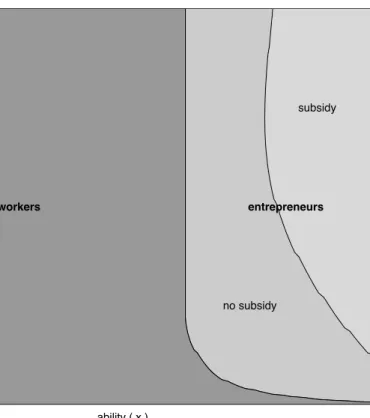
Figure 1 shows occupational choice in (aj, x) space for the economy in section
3.1 where ζ = 0.2w and τc = 1% per year. Lemma 1 and figure 1 indicate that
agents are workers when their entrepreneurial ability is low, i.e., x < x∗(w, r).
For x ≥ x∗(w, r) agents may become entrepreneurs, depending on whether or not
they are credit constrained. If initial wealth is very low, agents are workers even though their entrepreneurial ability is higher thanx∗(w, r). The negative association betweenaj
e(x;w, r) andxsuggests that managers with better managerial ability need
a lower level of initial wealth to run a firm. The lightest shaded area is the region in which agents apply for subsidized loans.
ability ( x ) w e a lt h ( b ) workers entrepreneurs subsidy no subsidy workers entrepreneurs subsidy no subsidy workers entrepreneurs subsidy no subsidy workers entrepreneurs subsidy no subsidy workers entrepreneurs subsidy no subsidy
Figure 1: Occupational choice.
Controlling for the agent’s net worth, aj, loan size varies positively with x and
we expect a positive relationship between entrepreneurial quality and the use of subsidized credit. The relationship between the use of subsidized credit and asset value, however, is ambiguous. On one hand, a large value of assets implies that restriction (11) does not bind and rich entrepreneurs rely less on outside finance and therefore on subsidized credit, since it is profitable to apply for such a loan if and only if lns(aj, x;w, r) > τζc. However, for high ability entrepreneurs the incentive compatibility constraint might bind and therefore a higher level of assets loosens the borrowing constraint and increases the option to use subsidized credit. Notice
that credit subsidies in our model help firms to expand at a faster rate and do not impose a restriction on size or promote small business. This is in contrast to the policy evaluated by Buera, Kaboski, and Shin (2012).
In order to investigate the effects of credit subsidies on occupational choice, firm size, borrowing, output and prices we must solve this general equilibrium model numerically. We first define an equilibrium.
2.2
Competitive equilibrium
Let Υ0 be the initial asset distribution that is exogenously given and let Υ be
the wealth (asset) distribution at some periodt, which evolves endogenously across periods. DefineP(aj, A) = Pr{aj0 ∈A|aj}as a non-stationary transition probability
function, which assigns a probability for an asset in t+ 1 to be at A for an agent with asset aj. The law of motion of the asset distribution is
Υ0 = J X j=1 Z P(aj, A)Υ(daj). (16)
In a competitive equilibrium, agents optimally solve their problems and all mar-kets clear. The agents’ optimal behavior was previously described in detail. It remains, therefore, to characterize the market equilibrium conditions. Since the consumption good is the numeraire, two market clearing conditions are required to determine the wage and interest rate in each period. The labor and capital market equilibrium equations are:
J X j=1 Z Z z∈E(w,r) n(x, aj;w, r)Υ(daj)Γ(dx) +Nc= J X j=1 Z Z z∈Ec(w,r) Υ(daj)Γ(dx), (17) J X j=1 Z Z z∈E(w,r) k(aj, x;w, r)Υ(daj)Γ(dx) +Kc= J X j=1 Z Z ajΥ(daj)Γ(dx). (18)
In addition, the government budget constraint is satisfied with equality, so that:
J X j=1 [ Z Z z∈E(w,r) τwwn(x, aj;w, r)Υ(daj)Γ(dx) + Z Z z∈Es(w,r) ζΥ(daj)Γ(dx)] = (19) J X j=1 Z Z z∈Es(w,r) τcl(x, aj;w, r)Υ(daj)Γ(dx) +g.
to manage the subsidized loan program. Alternatively, we could have assumed that this fixed cost is redistributed back to all households. In this case, the increase in the payroll tax rate, τw, to finance credit subsidies will be, in general, larger than in the case in which the fixed cost is assumed to be part of government revenue. Quantitatively results are roughly the same using the two approaches14 and for the sake of space we only report the simulations in which equation (19) is satisfied. Finally, assume that intermediation cost,η, is redistributed back to households:
J X j=1 Z Z trΥ(daj)Γ(dx) = J X j=1 Z Z z∈E(w,r) ηl(aj, x;w, r)Υ(daj)Γ(dx). (20)
In a similar model, Antunes, Cavalcanti, and Villamil (2008a) prove analytically the existence of a unique stationary equilibrium that is fully characterized by a time invariant asset distribution and associated equilibrium factor prices. They show that from any initial asset distribution and any interest rate, convergence to this unique invariant asset distribution occurs. They also describe a direct, non-parametric approach to compute the stationary solution.
3
Measurement
In order to study the quantitative effect of credit subsidies on entrepreneurship, economic development, inequality, and other variables, we must assign values for the model parameters. We calibrate to match key statistics in the United States, a well developed financial market with relatively small intermediation costs. Subsequently we will conduct counterfactual analyses where we fix the baseline parameters at the U.S. level, and then counterfactually feed in policies that correspond to Brazil, a country with repressed financial markets and large intermediation costs.
3.1
Calibration
The baseline model is calibrated so that the long run equilibrium matches some key
statistics of the U.S. economy. We assume that J = 9 and each model period is 5
years.15 As a result, each agent has a productive lifetime of 45 years. Assume that
the cumulative distribution of managerial ability is given by Γ(x) =x1 andx∈[0,1].
14The results are similar when ζis a pure deadweight loss.
15Results are not very different when J = 1 in the model, as in Galor and Zeira (1993). This is
because we re-calibrate the parameters of the model to match the same statistics of the baseline economy. In general financial frictions have a strong effect on output whenJ = 1, and if we were to changeJ but fix other parameters at the baseline the results would differ.
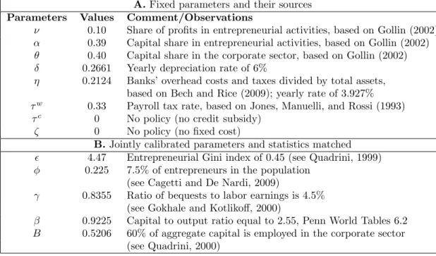
Table 1: U.S. parameter values, baseline economy. A time period is 5 years andJ = 9
A.Fixed parameters and their sources
Parameters Values Comment/Observations
ν 0.10 Share of profits in entrepreneurial activities, based on Gollin (2002)
α 0.39 Capital share in entrepreneurial activities, based on Gollin (2002)
θ 0.40 Capital share in the corporate sector, based on Gollin (2002)
δ 0.2661 Yearly depreciation rate of 6%
η 0.2124 Banks’ overhead costs and taxes divided by total assets, based on Bech and Rice (2009); yearly rate of 3.927%
τw 0.33 Payroll tax rate, based on Jones, Manuelli, and Rossi (1993)
τc 0 No policy (no credit subsidy)
ζ 0 No policy (no fixed cost)
B.Jointly calibrated parameters and statistics matched
4.47 Entrepreneurial Gini index of 0.45 (see Quadrini, 1999)
φ 0.225 7.5% of entrepreneurs in the population
(see Cagetti and De Nardi, 2009)
γ 0.8355 Ratio of bequests to labor earnings is 4.5% (see Gokhale and Kotlikoff, 2000)
β 0.9225 Capital to output ratio equal to 2.55, Penn World Tables 6.2
B 0.5206 60% of aggregate capital is employed in the corporate sector (see Quadrini, 2000)
When is one, entrepreneurial talent is uniformly distributed in the population. Whenis greater than one, the talent distribution is concentrated among low talent agents. Fourteen parameters must be determined: six for technology (θ, B, ν, α, δ, ), three for utility (σ, β, γ), and five institutional and policy parameters (φ, η, ζ, τw, τc).
Table 1 lists the value of each parameter in the baseline economy. Below we describe in detail how we assign each value.
We set ν and α so that in the entrepreneurial sector 55% of income is paid to labor, 35% is paid to remunerate capital, and 10% are profits.16 Therefore,ν = 0.1
and α = 0.39. In the corporate sector, we set θ = 0.40, which implies a capital
income share of 40%, consistent with Gollin (2002). We assume that the capital stock depreciates at a rate of 6% per year, a number used in the growth literature (e.g., Gourinchas and Jeanne, 2006). The coefficient of relative risk aversionσ is set at 2.0, consistent with micro evidence in Mehra and Prescott (1985). We estimateη directly. Bech and Rice (2009, page A88, table A.1) show that in the United States the average from 1999 to 2008 of banks’ non-interest expenses (overhead costs) over assets is about 3.365%. Bech and Rice (2009) also report that the average value for taxes over total assets paid by banks during the same period was 0.562%, which implies that the total level of intermediation costs is 3.927% per year. We set τw = 0.33 to match the average tax rate on labor income in the United States
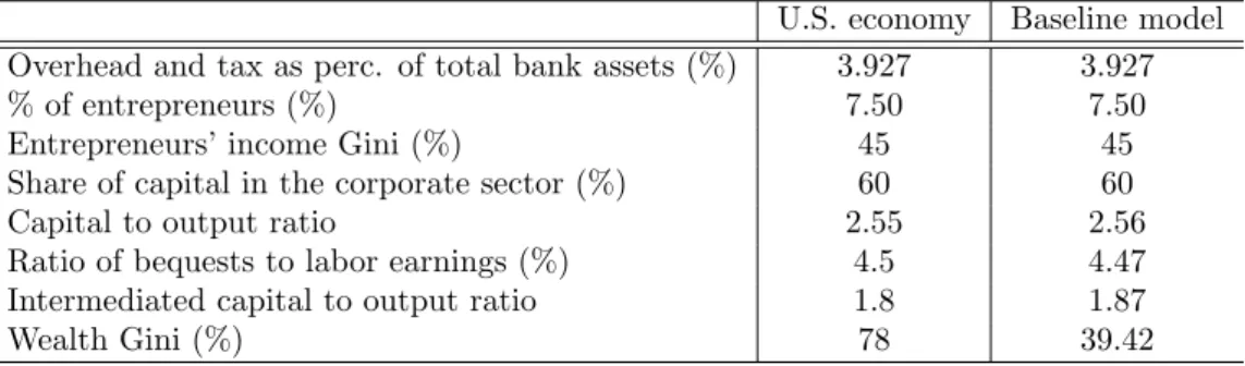
Table 2: Basic statistics, U.S. and baseline economy. Sources: International Financial Statistics database, Bech and Rice (2009), Cagetti and De Nardi (2009), Casta˜neda, D´ıaz-Gim´enez, and R´ıos-Rull (2003), Gokhale and Kotlikoff (2000), Heston, Summers, and Aten (2006), McGrattan and Prescott (2000), Quadrini (1999), Quadrini (2000).
U.S. economy Baseline model
Overhead and tax as perc. of total bank assets (%) 3.927 3.927
% of entrepreneurs (%) 7.50 7.50
Entrepreneurs’ income Gini (%) 45 45
Share of capital in the corporate sector (%) 60 60
Capital to output ratio 2.55 2.56
Ratio of bequests to labor earnings (%) 4.5 4.47
Intermediated capital to output ratio 1.8 1.87
Wealth Gini (%) 78 39.42
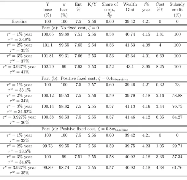
(cf., Jones, Manuelli, and Rossi, 1993). We first consider an economy with no credit subsides: τc= 0 andζ = 0.
The values of five remaining parameters must be determined: The productivity parameter of the corporate sector, B; the curvature of the entrepreneurial ability distribution,; the subjective discount factor,β; the altruism utility factor, γ; and the strength of financial contract enforcement,φ. These five parameters are chosen so that in the stationary equilibrium we match five key statistics of the United Sates economy: the capital to output ratio, which is equal to 2.55;17 the percent
of entrepreneurs over the total population, which is about 7.5% (see Cagetti and De Nardi, 2009); the Gini index of entrepreneurial earnings, which corresponds to roughly 45% (see Quadrini, 1999); 60% of aggregate capital is employed in the corporate sector (see Quadrini, 2000); and the ratio of bequests to labor earnings is roughly 4.5%, which is the number estimated by Gokhale and Kotlikoff (2000).
The model matches the U.S. economy fairly well along a number of dimensions that were calibrated (the first six statistics in table 2), as well as some statistics that were not calibrated, such as the level of intermediated capital to output ratio. McGrattan and Prescott (2000) report that the intermediated capital to output ratio in the United States is 1.8 and that corporations are the leading institutions of capital ownership. If we assume that most capital in the corporate sector is intermediated by either financial institutions, or by issuing bonds and stocks, our measure of intermediated capital is 1.87. The measure of intermediated capital in
17The estimated value of the capital to output ratio ranges from 2.5 (see Maddison, 1995) to
3 (see Cagetti and De Nardi, 2009). Using the Heston, Summers, and Aten (2012) Penn World Tables 7.1 and the inventory method, we construct the capital to output ratio for the United States and estimate it to be 2.55. The value forβ is 0.9225. Since the model period is 5 years, this implies that agents discount the future at a rate of about 1.63% per year.
the entrepreneurial sector is about 33% of output. Finally, the model does not match the wealth Gini well: the model predicts roughly 40%, while the data is 78% (see Casta˜neda, D´ıaz-Gim´enez, and R´ıos-Rull, 2003). Every worker receives the same equilibrium wage rate in the model economy, while in the data there is much more labor heterogeneity.18
3.2
Quantitative Experiments
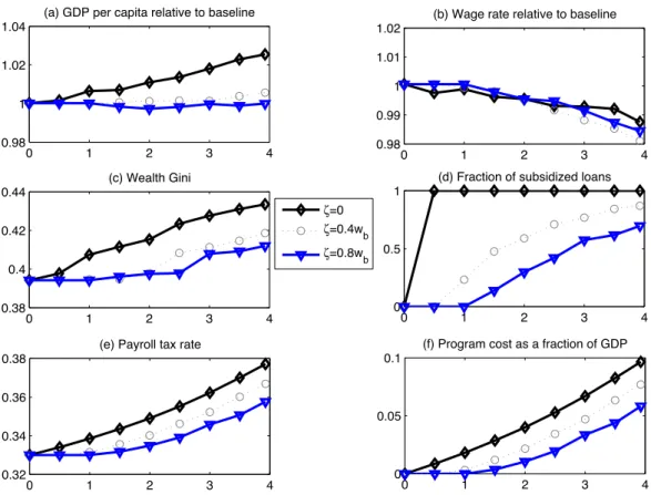
We now explore numerically how the equilibrium properties of the model change with benchmark variations in the credit subsidy policy. We examine the model’s predictions along six dimensions: output per capita as a fraction of the baseline value, the wage rate as a fraction of the baseline value, the wealth Gini coefficient, the fraction of subsidized loans, the payroll tax rate, and the cost of the program as a share of income. In appendix A, we provide a detailed table and explore the effects of credit subsidies on the following additional variables: the capital to output ratio, the fraction of entrepreneurs in the economy, the interest rate and entrepreneurs’ income Gini. All statistics correspond to the stationary equilibrium of the model.
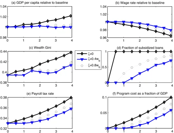
Figure 2 describes the model’s predictions as the value of the credit subsidy changes from 0 to a value such that the borrowing and deposit rates are the same. Recall (10), where (1 +r+η−τc1
s) is the interest rate on a bank loan, with fixed
application cost 1sζ. When τc = ζ = 0 the government does not offer the policy.
We evaluate the effects for values of fixed cost ζ, ranging from 0 (black solid line with a diamond marker) to costs up to 80% of the baseline wage (blue solid line with a triangle marker). Results for an intermediate value of ζ are displayed in the grey dotted line. When it is costless to apply all loans receive subsidies, and when ζ >0 subsidized loans are selected endogenously. As subsidy τc rises entrepreneurs increase the demand for loans for a given interest rate. This is a demand effect. If the economy is small and financially integrated in the world market, then the interest rate will not change. If there are restrictions on capital flow, this demand effect will push interest rates up. This in turn would decrease the profitability of entrepreneurial activity. This is a general equilibrium supply effect. In addition, larger loans increase entrepreneurial production, and the accumulation of capital, which decreases the interest rate in the long run. Therefore, the impact of credit subsidies on development is unclear. Notice also that the payroll tax rate must increase to balance the government budget constraint, which decreases labor demand and production.
18As is well known, labor income shocks can be added to increase the income and wealth Gini
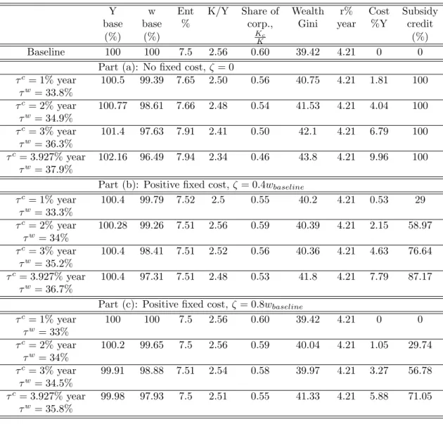
Figure 2(a) shows that in the baseline model, credit subsidies do not have a strong quantitative effect on output. When there is no fixed cost and credit subsidies increase from τc = 0 to τc = 3.927% per year, output per capita increases by less
than 3% in the long run;19 the wage rate decreases by about 1.3%; and wealth
inequality increases. The Gini coefficient for household wealth increases by more than 10%; the payroll tax rate increases sharply from 0.33 to 0.38 to balance the government budget constraint, since government spending increases by about 10 percentage points. When the fixed cost is positive, the effects of credit subsidies on all variables are similar to the baseline case where ζ = 0 but, in general, are quantitatively smaller; the positive effect on output and the negative effects on wages and government finances remain. Loan selection is endogenous and not all entrepreneurs benefit from the program. Our results show that the effects of credit subsidies on GDP are small, but they have non-negligible impacts on government finances and important distributional effects. Aggregate output does not change much, but there is an important compositional change: income is transferred from workers to entrepreneurs, and the latter remain a small part of the total labor force.20
Interestingly, in table 4 in appendix A we can see that although output increases, the capital to output ratio decreases in the long-run with credit subsidies. This implies that total factor productivity (TFP) must increase when the government subsidizes loans. In order to see this, observe that for a normalized population of 1, aggregate output is Y =T F P ×KαY, where α
Y is the capital share in income.
Therefore, Y = T F P
1
1−αY ×(K Y )
αY
1−αY. This suggests that the allocation of talent
improves in this economy, but there is a loss of income for workers.
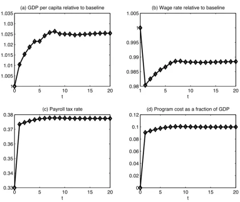
Figure 2 displays the long-run effects of credit subsidies. In order to investigate whether or not there is overshooting in the short-run in output and wages, such that long-run analysis underestimates the effects of credit subsidies on development, we calculate the transition from the baseline model to a model with positive credit subsidies. Figure 3 reports the transition of output, the wage rate, payroll tax rate, and the program cost as a share of income from the baseline model with no credit subsidies to a model in which there is no fixed cost to apply for subsidized loans and there is no spread between deposit and loan rates (i.e., τc = 3.927% and ζ = 0).21 Notice that output monotonically increases from the initial equilibrium to its final
19Whenζ= 0 the largest effect is atτc= 3.927% per year: output per capita increases 2.29%. 20In U.S. data, entrepreneurs are 7.5% of the labor force. In the experiment the share of
en-trepreneurs increases only slightly with credit subsidies: in the baseline with no fixed costs, it goes from 7.5% to 7.93% when credit subsidyτc changes from 0 to 3.927% per year. See panel (a) in table 4 in appendix A.
21Transitions for other experiments reported in Figure 2 follow a similar qualitative path. For
0 1 2 3 4 0.98
1 1.02 1.04
(a) GDP per capita relative to baseline
0 1 2 3 4 0.98 0.99 1 1.01 1.02
(b) Wage rate relative to baseline
0 1 2 3 4 0.38 0.4 0.42 0.44 (c) Wealth Gini 0 1 2 3 4 0 0.5 1
(d) Fraction of subsidized loans
0 1 2 3 4
0.32 0.34 0.36 0.38
(e) Payroll tax rate
0 1 2 3 4
0 0.05 0.1
(f) Program cost as a fraction of GDP
ζ=0
ζ=0.4wb
ζ=0.8wb
Figure 2: Economy with endogenous interest rate, distortionary labor tax, and subsidy
τcraised from 0 to 3.927%. Different lines indicate different fixed costs,ζ = 0, .4wb, .8wb.
Long run effects of credit subsidies on: (a) GDP per capita relative to the baseline; (b) wage rate relative to the baseline; (c) wealth Gini index; (d) fraction of subsidized loans; (e) payroll tax rate; and (f) total subsidized loans over GDP.
long-run level, while the wage rate first decreases and then increases to a level below the long-run level.22 Clearly, the long-run analysis does not underestimate the transitional effects of credit subsidies on investment and output. For the wage rate, the long-run analysis provides a lower bound for the negative effect of credit subsidies on wages. Given that, we focus on the long-run effects of credit subsidies. The general equilibrium effect might offset the demand effect of credit subsi-dies. In order to understand the role of general equilibrium price changes in driving results, we also consider an economy that is financially integrated in international capital markets. In this case, financial intermediaries have access to an elastic sup-ply of funds and the interest rate is exogenously given; the model indicates it is 4.21% per year under baseline parameters. The effects of credit subsidies can differ greatly when the interest rate is exogenous or endogenous, see Castro, Clementi, and
22The intuition is that with the introduction of the program there is a demand for subsidized loans
and the tax rate must increase to balance the budget, which decreases labor demand. However, there is more investment and capital accumulation, and the marginal product of labor increases.
0 5 10 15 20 1 1.005 1.01 1.015 1.02 1.025 1.03 1.035 t
(a) GDP per capita relative to baseline
1 5 10 15 20 0.98 0.985 0.99 0.995 1 1.005 t
(b) Wage rate relative to baseline
0 5 10 15 20 0.33 0.34 0.35 0.36 0.37 0.38 t (c) Payroll tax rate
0 5 10 15 20 0 0.02 0.04 0.06 0.08 0.1 0.12
(d) Program cost as a fraction of GDP
t
Figure 3: Economy with endogenous interest rate and distortionary labor tax: Transition from the baseline to an equilibrium with all parameters equal to the baseline, except
τc= 3.927% per year. Long run effects of credit subsidies on: (a) GDP per capita relative to the baseline; (b) wage rate relative to the baseline; (c) payroll tax rate; and (d) total subsidized loans over GDP.
MacDonald (2004) and Antunes, Cavalcanti, and Villamil (2008b) where the general equilibrium effect is quantitatively important in analyzes of financial reforms that improve creditors’ rights. Figure 4 shows the model’s predictions in an economy completely open to capital flows as the value of the credit subsidy rises from 0 to a value such that the borrowing and deposit rates are the same for different levels of the fixed cost (see also table 5 in appendix A).
Figure 4 shows that the relationship between the selected variables and credit subsidies has the same pattern whether the interest rate is endogenous or exogenous. The output effect is slightly smaller than in the case with an endogenous interest rate, but the quantitative difference is small. The maximum effect on output occurs when τc = 3.927% per year and the fixed cost, ζ, is null. In this case, output increases by 2.16% relative to the baseline. Notice, however, that the effects on government expenditures are still strong. The wage rate decreases by 3.5%. Overall, the policies we consider have no major quantitative difference on wages and the interest rate
does not change much, see Table 4 in Appendix A.23 Notice, however, that the
0 1 2 3 4 0.98
1 1.02 1.04
(a) GDP per capita relative to baseline
0 1 2 3 4 0.96 0.98 1 1.02 1.04
(b) Wage rate relative to baseline
0 1 2 3 4 0.38 0.4 0.42 0.44 (c) Wealth Gini 0 1 2 3 4 0 0.5 1
(d) Fraction of subsidized loans
0 1 2 3 4
0.32 0.34 0.36 0.38
(e) Payroll tax rate
0 1 2 3 4
0 0.05 0.1
(f) Program cost as a fraction of GDP ζ=0
ζ=0.4wb ζ=0.8wb
Figure 4: Economy with exogenous interest rate and distortionary labor tax. Long run effects of credit subsidies on: (a) GDP per capita relative to the baseline; (b) wage rate relative to the baseline; (c) wealth Gini index; (d) Fraction of subsidized loans; (e) payroll tax rate; and (f) total subsidized loans over GDP. Different lines correspond to economies with different levels of the fixed cost,ζ.
positive effects on TFP are stronger since the capital to output ratio decreases more than the case with an endogenous interest rate.
We also study the role of the payroll tax in shaping results, since in our baseline model the program is financed by a payroll taxτw. Consider the model in Section 2, but assume that the program is financed through a lump-sum tax on all households. Figure 5 (see also Table 6 in Appendix A) shows that in this case output per capita increases and the wage rate decreases in the long-run. In the experiment with no
fixed costs, output per capita and the wage rate change by 2.38% and −2.26%,
respectively, when credit subsidy, τc, changes from 0 to 3.927% per year. Total
subsidies as a fraction of income still increase by roughly 10 percentage points, which implies a transfer of resources from households to a small fraction of entrepreneurs.24 effect pushes interest rates up, more production and capital accumulation decreases the marginal productivity of capital and therefore decreases the interest rate. In addition, the payroll tax rate increases significantly and this decreases the demand for capital and production.
Net wage income, wages minus the lump-sum tax, decreases by about 4% relative to the baseline. Thus, the results are similar under lump sum taxation.
0 1 2 3 4
0.98 1 1.02 1.04
(a) GDP per capita relative to baseline
0 1 2 3 4 0.96 0.98 1 1.02 1.04
(b) Wage rate relative to baseline
0 1 2 3 4 0.38 0.4 0.42 0.44 (c) Wealth Gini 0 1 2 3 4 0 0.5 1
(d) Fraction of subsidized loans
0 1 2 3 4
0.32 0.34 0.36 0.38
(e) Payroll tax rate
0 1 2 3 4
0 0.05 0.1
(f) Program cost as a fraction of GDP
ζ=0
ζ=0.4w
b
ζ=0.8wb
Figure 5: Economy with endogenous interest rate, lump-sum tax, andτcraised from 0 to 3.927. Long run effects of credit subsidies on: (a) GDP per capita relative to the baseline; (b) wage rate relative to the baseline; (c) wealth Gini index; (d) fraction of subsidized loans; (e) Net wage relative to baseline; and (f) total subsidized loans over GDP. Different lines correspond to economies with different levels of the fixed cost,ζ.
3.3
Counterfactual Analysis: Brazil
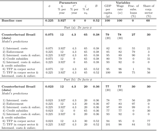
The previous experiments describe quantitative properties of the model for system-atic variations in the level of credit subsidies, τc, and fixed cost, ζ. We now use independent estimates of intermediation costs, contract enforcement and subsidy policy for Brazil, keeping the other parameters at the U.S. level. This counterfac-tual exercise gives an estimate of how much of the difference in output per worker between Brazil and the U.S. can be accounted for by differences in financial market imperfections and credit market policies. According to the Heston, Summers, and Aten (2012), U.S. output per capita is 5 times larger than Brazil’s output per capita. The counterfactual exercises show what the level of U.S. output per worker would be
if financial contract enforcement, intermediation costs, and interest subsidy policy were the same as in Brazil.25
Beck, Demirg¨u¸c-Kunt, and Levine (2009) report that the ratio of banks’ over-head costs to total assets is about 11% in Brazil. In addition, Demirg¨u¸c-Kunt and Huizinga (1999) show that the value for taxes over total assets paid by banks is roughly 1%. Therefore, we setη such that the annual value of intermediation costs is 12%.26 As in Antunes, Cavalcanti, and Villamil (2008b), two methods are used to
assess enforcement parameterφ: a de juris measure based on the written law and a de facto measure to account for how laws are likely to be enforced. For the de juris measure we use a legal rights index which indicates the degree to which collateral and bankruptcy laws facilitate lending. The index ranges from 0 to 10, with higher scores indicating that collateral and bankruptcy laws are better designed to promote access to credit. To determine the parameter estimate for φ, multiply the ratio of the legal rights index of Brazil (3) to the U.S. value (9) by the baselineφ= 0.225.27 The corresponding value for Brazil is φ= 39 ×0.225 = 0.075.
The written law is only part of investors’ legal protection. Another part is the overall quality of the rule of law in the country, as this determines how the written law is enforced in practice. We also define investor protection by the previous legal rights index times a rule of law indicator. The rule of law index computed by Kaufmann, Kraay, and Mastruzzi (2003) measures the degree to which laws are enforced in society.28 According to this index, the U.S. has a score of 8.16 while
Brazil’s score is 2.50. Investor protection between the U.S. and Brazil now varies by a factor of 10, while with the de juris measure the difference in investor protection is a factor of 3.
We now set the value for policy parameter τc and institutional parameter ζ to
values used by the Brazilian National Development Bank (BNDES), the main sup-plier of subsidized credit in Brazil. BNDES resources come mainly from workers’
25We are not arguing that other parameters in Brazil are the same as those observed in the U.S.
The goal is to isolate the effects of intermediation costs, enforcement, and credit subsidies in a pure counterfactual exercise. In a technical note, we calibrate all parameters to match the Brazilian economy, seehttp://sites.google.com/site/tiagovcavalcanti/research-1. We consider several cases, including when there is a cap on the interest rate that financial intermediaries can charge on subsidized loans. The effects of credit subsidies on development are robust to different calibrations of the model and are consistent with the findings reported here.
26The interest margin in Brazil reported by Beck, Demirg¨u¸c-Kunt, and Levine (2009) is about
14%. However, the net interest margin also contains loan loss provisions and after tax bank profits, which are not explicitly modeled here.
27We implicitly assume that the relationship between the index and the parameter is linear, at
least locally. This is an approximation, and we know that the polar cases coincide.
28We use the 2010 rule of law index, which varies from -2.5 to 2.5, normalized to a 0 to 10
contributions and loans from the Brazilian Treasury at a rate below the Central Bank interest rate. In 2008-2010, for instance, the yearly nominal interest paid by government bonds (Selic) was about 12%, while the government lent to BNDES at about 6%. BNDES has no branches and it provides credit mostly through commer-cial and regional development banks,29 which access BNDES resources at low rates that they pass on to firms. The final component in BNDES credit lines is an interest rate spread charged by BNDES of about 1.73 percentage points in 2009-2010 (aver-age value, see BNDES, 2010) and a financial intermediaries spread.30 Therefore, we
assume that BNDES provides an annualized interest rate subsidy of 4.3 percentage points on loans, so thatτc= 0.2343. That is, Selic 12% - Lend 6% - Spread 1.7% =
4.3% per year, the model period is 5 years, and 5(4.3%) = 23.43%.
According to Sant’Anna, Bor¸ca-Junior, and de Araujo (2009), BNDES is respon-sible for about 18% of all credit in Brazil. The World Development Indicators report that private credit over output in Brazil has been growing recently and in 2008 it reached about 45% of GDP. However, not all loans go to firms. Sant’Anna, Bor¸ca-Junior, and de Araujo (2009) report that about 35% of the total credit in Brazil finances either family consumption or housing. Therefore, credit to production is about 29% of income and BNDES loans account for about 27% of all productive credit.31 We thus calibrate ζ so that the share of subsidized credit is about 27
percent of all credit in our model economy.
We also must adjust the TFP parameter of the production function in the cor-porate sector, such that the share of capital in the corcor-porate sector is similar to the one in Brazil. Otherwise, with the financial repression observed in Brazil (values for φ and η), the size of the corporate sector will be too large relative to the level in Brazil. We define the corporate sector as all firms listed in the Brazilian stock market. BMF & BOVESPA data32 indicate that total permanent assets of listed
firms in Brazil are about 0.66 of GDP. Since the capital to output ratio is 2.2,33 this
implies that about 30% of the capital is employed in the corporate sector in Brazil. Therefore, we adjust TFP parameterB such that the capital share of the corporate
29In some credit programs borrowers can apply directly to BNDES, but the majority of loans
are through commercial and regional development banks. See Ribeiro and DeNegri (2010) and Ottaviano and de Sousa (2008), for more details about how BNDES operates and its credit lines.
30BNDES loans have a longer term than other types of credit, but require large collateral. The
loan maturity for firms in general is within 60 months, the time period of our model economy.
31BNDES also finances the corporate sector (see Torres-Filho, 2009) where the marginal product
of capital is lower than for some credit constrained entrepreneurs. In our model, all credit subsidies go to entrepreneurs and therefore our results are an upper bound of the effects of credit subsidies in Brazil on output.
32Available at http://www.bmfbovespa.com.br/
33Using the Heston, Summers, and Aten (2012) Penn World Tables 7.1 and the inventory method,
sector is equal to 30%.
Table 3: Empirical Data and Model Predictions for Brazil.
Parameters Variables
φ η τc ζ B GDP Wage Frac. of Share of % per % per % of per rate subs. corp.
year year wb capita (w) loans sector
(y) (%) (%)
Baseline case 0.225 3.927 0 0 0.52 100 100 0 60
Part (a):De jurisφ
Counterfactual Brazil 0.075 12 4.3 65 0.38 79 78 27 30
(data) (20) (30)
Model’s predictions
1) Intermed. costs 0.075 3.927 4.3 65 0.38 82 81 55 21 2) Enforcement 0.225 12 4.3 65 0.38 85 82 79 3 3) Intermed. costs & enforc. 0.225 3.927 4.3 65 0.38 95 89 90 0 4) Credit subsidies 0.075 12 0 65 0.38 80 79 0 31 5) Intermed. costs & enforc. 0.225 3.927 0 65 0.38 93 92 0 0 & credit subsidies
6) TFP in corpor sector 0.075 12 4.3 65 0.52 95 96 1 76 7) TFP in corpor sector & 0.225 3.927 4.3 65 0.52 100 99 75 56 Intermed. costs & enforc.
Part (b): De factoφ Counterfactual Brazil 0.023 12 4.3 20 0.36 77 77 30 30 (data) (20) (30) Model’s predictions 1) Intermed. costs 0.023 3.927 4.3 20 0.36 78 77 56 29 2) Enforcement 0.225 12 4.3 20 0.36 87 83 97 0 3) Intermed. costs & enforc. 0.225 3.927 4.3 20 0.36 97 89 99 0 4) Credit subsidies 0.023 12 0 65 0.36 77 77 0 30 5) Intermed. costs & enforc. 0.225 3.927 0 20 0.36 93 92 0 0 & credit subsidies
6) TFP in corpor sector 0.023 12 4.3 30 0.52 94 95 0 77 7) TFP in corpor sector & 0.225 3.927 4.3 20 0.52 101 98 84 53 Intermed. costs & enforc.
Table 3 contains the results of the counterfactual exercises. Part (a) reports exercises in which we use the de juris measure for φ, while Part (b) uses the de facto measure for φ. The first row in bold displays the key parameters of the model related to the functioning of the financial market (φ,η,τc,ζ,B) of the U.S. economy
along with the normalized value of output per capita and wage rate, and values for the share of capital in the corporate sector. The second row reports the value of enforcement (φ), intermediation costs (η), and credit policies (τc and ζ) for Brazil.
It also displays the value of the TFP factor (B) in the corporate sector, which would match the share of capital in Brazil’s corporate sector data.34 Finally, it contains
the output per capita and the wage rate relative to the baseline generated by the
34The equilibrium real interest rate is smaller than the one observed in the U.S. since the financial
model and the values observed in the data (in parentheses).35 Notice that output
per capita in Brazil relative to the U.S. level is roughly 20 percent, while in the model it is 79 percent withφ de juris and 77 percent with φ de facto.36 Therefore, differences in the functioning of the financial sector and in the TFP parameter of the corporate sector explain roughly 25-29 percent of the difference in output per capita between Brazil and the U.S.
Next, we perform several counterfactual exercises to study the role of each factor in explaining differences in income levels. In the fourth exercise, for instance, we cut interest rate subsidies from the Brazilian level of 4.3 percentage points per year to zero. Output and wages are unchanged, whether we use thede juris or de facto measure forφ. Therefore, the credit subsidy policy in Brazil does not have a positive effect on aggregate output and wages and does not explain any of the difference in
output per capita between the two economies. The policy has a non-negligible
impact on government finances, since the cost of the program in our counterfactual models is around 0.7 percent of income.
For comparison, in experiment 2, we keep all parameters the same as in the Brazilian counterfactual case, reported in the second row of Table 3, but now exoge-nously change the value of enforcement parameter φ back to the value observed in the U.S. Recall thatφis a penalty which entrepreneurs face when they do not honor their promises to repay their debt, reflecting the strength of contract enforcement in the economy. A smallerφ corresponds to a low level of enforcement of financial contracts, while when φ goes up it implies an increase in the level of enforcement. For the case of φ de juris, output per capita would increase by 6 percentage points
or roughly 7%, and the wage rate would increase by 4%. When we consider φ de
facto, output and the wage rate increase by 10 and 6 percentage points, respectively. Therefore, the enforcement parameter alone explains 9-12.5% of the difference in in-come per capita between the U.S. and Brazil.
When both intermediation costs and enforcement are changed to the level ob-served in the U.S. (experiment 3), then output per capita increases by 6 and 20 percentage points, depending on the measure of enforcement used. The effect on output is stronger when we use the de facto measure, and enforcement of financial contracts and intermediation costs explain about 25 percent of the difference in
out-35Output per capita is taken from Heston, Summers, and Aten (2012) and corresponds
to the average value from 2008 to 2010 of the series “PPP Converted GDP Per Capita (Chain Series), at 2005 constant prices”. For the wage rate, we use the 2010 hourly com-pensation costs in manufacturing provided by the US Bureau of Labor Statistics (BLS). See: http://www.bls.gov/news.release/pdf/ichcc.pdf.
36The wage rate in the model with thede facto φ is equal to 77 percent of the U.S. wage rate.
put per capita between Brazil and the U.S. Observe that in experiment 3 the effect on the wage rate is not as strong as the effect on output. The reason is that when enforcement of financial contracts improves from the level of Brazil to the level of the U.S., financial intermediaries make more loans and the share of subsidized loans increases. Then, the payroll tax rate must increase, which decreases labor demand. In experiment 5, we change the level of enforcement and intermediary costs to the level observed in the U.S., but we also cut all interest subsidies. In this case output and the wage rate increase by almost the same amount.37
Together, differences in productivity in the corporate sector, enforcement of fi-nancial contracts and intermediation costs are able to explain 25 percent of the dif-ference in output per capita between the U.S. and Brazil, but credit subsidies have no important effect on output. These experiments suggest that, for realistic changes in the legal protection of contracts and intermediation costs, considerable gains in output and wages could occur. These changes are much larger than changes from credit subsidies. The model simulations are also consistent with empirical evidence on interest credit subsidies and development,38 and the general equilibrium model
makes clear the forces that drive the outcomes (see Azariadis and Kaas (2007)).
4
Concluding remarks
This paper studies the quantitative effects of interest rate credit subsidies on out-put, wages, and inequality in a standard model of economic development with credit market imperfections. We calibrate the model to mimic key features of the United States economy and show that interest rate subsidies have no significant quantitative effect on output per capita, but can have negative effects on wages. Such subsidies work as transfers from workers to a small group of entrepreneurs. Consistent with empirical evidence, our results suggest that providing interest rate subsidies of the type we study is not an effective way to reduce the underinvestment problem that can result from capital market frictions. Countries should focus on financial reforms that improve the functioning of financial and credit markets directly, such as reforms
37Output increases by 14 and 16 percentage points, while the wage rate increases by 14 and 15
percentage points, depending on which measure of enforcement is used.
38Using manufacturing industry data, Lee (1996) shows that cheap credit programs had no
significant effect on capital accumulation or TFP in Korea. Using firm level data, Ribeiro and DeNegri’s (2009) estimates suggest that BNDES cheap credit had limited effects on TFP growth in Brazil. Using value added per worker, Ottaviano and de Sousa (2008) find that BNDES loans increase productivity only for large projects but not for small loans and the aggregate effect is not statistically different from zero. Lazzarini and Musacchio (2011) find a significant effect of BNDES minority equity stakes on firm performance (ROA), which they attribute to weaker capital constraints for publicly traded companies when the development bank is a shareholder.