Help File Version

(1)

Help File

Version 1.0.14

By

engineering@optimumg.com

www.optimumg.com

(2)

Welcome

Thank you for purchasing OptimumT the new benchmark in tire model fitting and analy-sis. This help file contains information about all the functions and features of OptimumT. Included in this help file are:

• Information on how to use OptimumT

• Special Features in OptimumT

(3)

Feedback

OptimumT is a continually developing program and we give high regard to any sugges-tions, comments, complaints or criticisms that OptimumT users might have. Please contact us at engineering@optimumg.com and we will work to improve OptimumT based on your feedback.

Features Coming Soon

The following is a list of features that will be available in future updates. Please contact us if you have any suggestions on other features that should be included in OptimumT in the future.

• Additional Tire Models

• Import and Export from TYDEX Files

• Automated Reports

(4)

Introduction

Through OptimumG’s consulting and seminar services, it identified tire data analysis and model fitting as an important, but often neglected area of vehicle dynamics. Therefore, OptimumT was created from OptimumG’s extensive knowledge and experience in testing, analysis, and development of vehicle tires and suspension systems. OptimumT is a convenient and intuitive software package that allows users to perform advanced tire data analysis, visualization, and model fitting.

Pacejka ’96, 2002, and 2006 tire models are available in OptimumT. Simpler Brush and Fiala models are also included. The models can be manually inputted, imported, or fit to raw tire data. The model fitting procedure is very fast and efficient partially due to the data processing tools incorporated into the software. All aspects of the tire models can be easily compared to the raw tire data to ensure accuracy. OptimumT also allows adjustment of the tire models if necessary and includes scaling factors for the Pacejka models. These features ensure that the tire models created will accurately correlate to data collected from the road or race track. These tire models, as well as the processed data, can be exported from OptimumT to a variety of file formats.

OptimumT is also a very powerful data visualization tool. It has the capability to display tire models and raw tire data in a user friendly but extremely powerful graphing utility. It features 2D and 3D graphing of over 30 different tire parameters. The ability to create surface plots and crossed line graphs allows the user to be able to easily create sophisticated graphs, like tire friction ellipses. The graphs can be further enhanced by including the effect of many different parameters including vertical load, inclination angle, and inflation pressure. These graphs can be easily copied or directly printed from the OptimumT interface to be included in other projects or reports. The data from these graphs can also be exported for further analysis.

(9)

Installation Requirements

Hardware Requirements

Processor

• IntelR Pentium 4TM, IntelR XeonTM, and IntelR CoreTM • AMDR AthlonTM, AMDR OpteronTM, and AMDR TurionTM

Memory

• Minimum: 512MB RAM

• Recommended: 1GB RAM or more

• Virtual Memory recommended to be twice the amount of RAM

Storage

• Free space of at least 100MB. Includes installation of OptimumTR and required

soft-ware components (see below)

Display Adapter

• Minimum: MicrosoftR DirectXR 9.0c capable graphics card with 32MB RAM • Recommended: DirectXR 9.0c capable NVIDIAR GeForceR or ATIR RadeonR

(10)

Display Unit

• Minimum: 15" Screen with resolution of 1024 x 768 pixels

• Recommended: 19" Screen with resolution of 1280 x 1024 pixels

Other

• Mouse or other pointing device

Software Requirements

Operating System

• MicrosoftR WindowsR XP (32 or 64bit) or MicrosoftR WindowsR Vista (32 or

64bit) or MicrosoftR WindowsR 7 (32 or 64bit)

Required Software Components

• MicrosoftR .NETR Framework 2.0 or higher

Other

(11)

License

Moving License

If the license needs to be moved to another computer this can be done through OptimumT. The two computers will both need to have an internet connection.

To move a license to another computer:

• Launch OptimumT.

• From the project screen select the Help menu and click Deactivate License.

• Click Yes in the Deactivate License message box.

• Click Deactivate in the Web Activation message box.

The "Online Deactivation was successful" message box will appear once the license has been deactivated. OptimumT can know be installed on another computer using the same license key.

License Viewer

The license viewer shows the status of the current license and allows the user to enter a new time license. Once OptimumT is installed the license viewer can be accessed through the Windows start menu. It will be located in the OptimumT folder. A new OptimumT time license can be activated by pressing the Activation Key button in the lower left corner of the license viewer. Then the new license key can be inputted and activated.

(12)

to trademarks or service marks of OptimumG. For more information regarding the rights and limitations of the OptimumT License please refer to the End-User License Agreement (EULA).

(13)

Chapter 1 Screen Layout

When OptimumT is opened the project screen will initially appear as shown in Figure 1.1. From this screen the user can either choose to open an existing project or create a new project. Once one of these is selected the primary OptimumT screen layout will be displayed.

Figure 1.1: Project Screen

The OptimumT screen layout is shown in Figure 1.2. The screen is divided into three basic sections:

(14)

• The data entry form

• The worksheets and the associated worksheet tabs

Figure 1.2: Screen Layout

1.1 Tire Project Tree

The tire project tree contains all the raw data, tire models, and scaling factors contained within the OptimumT project. Raw data and tire models are organized by the tire item. The tire items can be seen more closely in Figure 1.3.

(15)

Figure 1.3: Project Tree

The item type in the project tree can be identified by the icon to the left of the item. In Figure 1.3, the first item in the list is a tire. The tire item is like a folder that contains other items in the project. Both raw data and tire models must be associated with a tire item, so this must be the first item added to a new project. This allows data and models from the same tire or construction to be grouped together.

Raw Data

In Figure 1.3, the first two items in the project tree under Tire A are raw data. The icon for the second item, Combined Data, has a large red "C" in it to indicate that the collapsed data is being used. Data collapsing will be explained in section 2.3.

Tire Models

The third and fourth items in this project tree are tire models. The next two items are also tire models but the red "S" in the upper right corner of the icon indicates that a scaling factor has been applied to them.

(16)

Scaling Factors

The final item is a Pacejka scaling factor. These allow the model to be adjusted without making any changes to the model coefficients. Scaling factors are discussed in more detail in section 3.3.2.

Like the tire item when any of the raw data, tire models, or scaling factors is clicked additional information and functionality related to the selected item will appear in the data entry form. The small color squares in the lower right corner of the icons indicate the color in which the data or model will be displayed when it is graphed. To graph a specific tire model or raw data set, check the box next to the item in the project tree (graphing is covered in section 4).By right clicking on an item you can rename, delete, or copy it as well as perform other operations on it that will be discussed in later sections.

To add items to the project, the buttons above the project tree can be used. Figure 1.4 shows these buttons. The three buttons furthest to the right will only be enabled when an item in the project tree is selected.

Figure 1.4: Project Tree Buttons

1.2 Data Entry Form

When an item in the project tree is clicked on, a data entry form corresponding to the project item will appear in the data entry area. Note that the name of the project item or its icon must be clicked on. Clicking on the checkbox next to the item in the project tree will not bring up the data entry form, but will change whether or not the item is to be graphed. Figure 1.5 shows an example of the data entry form. This information appears when a tire item is selected in the project tree. Information about the tire size, manufacturing, and testing procedure can be stored here.

(17)

If the raw data, tire model, or scaling factor items are selected the information in the data entry area will change to reflect these items. The tire model coefficients are also contained in this form. If a graph is clicked on, the graph setup form for that specific graph will appear in the data entry area. The data entry forms will be discussed in more detail in the chapters corresponding to these specific items.

Figure 1.5: Tire Item Data Entry Form

1.3 Worksheets

(18)

Alternatively, worksheets can be added by right-clicking on the worksheet or the worksheet tabs and selecting New Worksheet.

Worksheets can be renamed by right-clicking on the worksheet and choosing Rename Work-sheet. A worksheet can be deleted (and all the graphs on that worksheet) by choosingDelete Worksheet from the menu that appears when you right-click on a worksheet. Note that you cannot undo a delete operation.

(19)

Chapter 2 Raw Tire Data

The raw data item in the project tree contains the imported data and provides some tools for manipulating the data. These tools allow the data to be quickly and conveniently viewed and fitted to tire models.

The raw data form, shown in Figure 2.1, is displayed when a raw data item in the project tree is clicked on. This form has a place to store comments about the test data contained in the item. It also contains theData CroppingandData Collapsing tools. TheData Cropping

tool allows user to easily view and eradicate erroneous or undesired data from the raw data. The Data Collapsing tool removes hysteresis from the data and separates the data into sets depending on the conditions that the tire was tested at. Once the data has been collapsed a summary of the separated data sets will appear in the table in the raw data from. The

Model Fitting tool in this section allows you to fit the raw or collapsed data to a tire model. Tire model fitting will be covered in more detail in section 3.

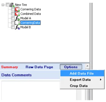
The Options button at the top of the raw data form allows you to add another data file, export the tire data, or access theData Cropping tool. A more detailed description of these operations is included in this section. The Data Comments allow the user to enter notes and information about the data. This information will be saved with the raw data in OptimumT.

(20)

(21)

2.1 Importing Data

When the Add Raw Data button above the project tree is clicked on, an open file window will appear. OptimumT can open either a .rtd file, which is the OptimumT binary format for tire data, or a CSV or ASCII file with .csv or .dat file extensions. Files with no extension are assumed to be CSV/ASCII files.

If a .rtd file is opened, the data will be automatically imported in the correct format and coordinate system. No further actions are required by the user.

If a CSV or ASCII file is selected a dialog box as shown in Figure 2.2 will open. In this box the the file properties can be specified. The character that separates the columns in the file and then the character that represents the decimal point should be selected. Multiple column separators can be selected if different file formats are to be used.

Figure 2.2: CSV Import Options

If a CSV or ASCII file is opened, the data import wizard, shown in Figure 2.3, will appear. In this window the user specifies what quantity each column of raw data contains (i.e. SA, SR, Fx, etc) and the unit for that quantity. At the bottom of the dialog box, default values for quantities that are missing from the data can be specified. For example, if inflation pressure was not recorded in the test, the user could manually enter a constant inflation pressure to be included in the data. The coordinate system that the data was collected also needs to be specified.

(22)

Figure 2.3: Data Import Wizard

This process can be automated by using the import template feature at the top of Figure 2.1. The template to be used is chosen through the CSV Import Template Selection dropdown box. It can be seen in the figure that currently Template 1 is selected. New import templates can easily be created and saved. First the data quantities, units, and coordinate system are specified. Then to save this as an import template, click the Save as New Template button. Import templates can also be modified and saved by using the Save Template button. Typically tire data provides the force and moments at the center of the tire contact patch. However sometimes, especially with wheel force transducer data, it will be the force and moments at the wheel center. Therefore theData in Hub-centered coordinate framecheckbox should be selected. Then OptimumT will transform the force and moment data to the center of the contact patch. If this is the case theRotate coordinate system by inclination angle can also be selected. This should be done if the coordinate system that the force and moments were measured in are fixed to the wheel. In this case the vertical force would be in the same direction as the inclination angle and not perpendicular to the ground. Therefore if this option is selected OptimumT will transform the forces and moments to a ground fixed coordinate system.

(23)

Figure 2.4: Adding more data to a data set that has already been imported

Once all of the column definitions have been assigned pressing the Next button will show a preview of the data to be imported. If the data to be imported is correct, clicking on Finish will import the data into OptimumT.

Generally different sets of raw data should be imported into OptimumT as separate files. However multiple test files can be imported and combined in OptimumT. This can be achieved in two ways. If the files are in exactly the same format, simply select both files at the same time (use the shift or ctrl keys to choose more than one file). The import wizard will appear for the first file and the other files will be imported with exactly the same settings. If the files are in different formate, multiple import into the same data item is done by importing the first data set as would normally be done. After this is completed, click on the data set in the project tree. Then select Add Data in the Options button in the upper right corner of the raw data form (see Figure 2.4). This will open the same CSV Import Wizard that was used previously. Follow the same steps as before and the data will be added to the previously imported set.

2.2 Data Cropping

Data cropping allows the user to remove any unwanted or unnecessary data. Often in tire tests the data from conditioning or warm up procedures is included in the data file. This data can be easily removed in OptimumT. The raw data can be cropped by selecting Crop Data under the Options button on the top of the raw data form. This will open the Crop

(24)

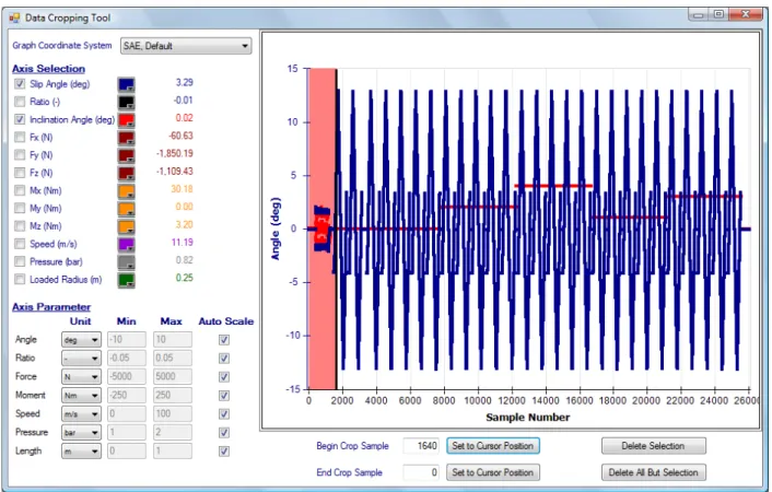
the left. In the figure slip angle is represented by the blue line and the inclination angle by the red line. By clicking on the boxes to the right of the properties the color of the property can be changed. The values to the right of this correspond to the data values at the location of the black line on the graph. At the bottom the units of the data and the axis ranges can be changed.

Figure 2.5: Data Cropping Tool

As can be seen at the beginning and end of the run extra data exists that is not necessary. The data to be removed can be selected by entering the beginning and ending sample numbers in the Begin Crop Sample and End Crop Sample textboxes at the bottom of the window. Alternatively the vertical black line on the graph can be dragged to the point where the data should be cropped. Pressing the corresponding Set button defines the beginning or ending sample number. The background of the selected data will be pink. Then theDelete Selection or Delete All But Selection buttons can be clicked to remove the selected data. Figure 2.6 displays the data from Figure 2.5 after it has been cropped. As can be seen only the relevant test data remains. When the Crop Data is closed the program will return to the primary OptimumT screen with cropped data.

(25)

Figure 2.6: Cropped Data

2.2.1 Data Cropping Templates

To simplify the task of repetitively cropping data, templates can be set up. Crop templates record the beginning and ending sample number of each section deleted. The same actions can be applied to another data file. The file on which a template is used must be at least on long as the largest ending sample number in the template. A warning will be displayed if the crop template was created for a data file with a different number of samples than the one its being applied to.

To record a crop template, simply crop a data file as usual. Once this is done, click on the "Save As" button next to Crop Template. Enter a name for the template and click on Save. To use a crop template, open the Data Cropping Tool (see Section 2.2) and choose the desired crop template from the Crop Templates List.

(26)

2.3 Data Collapsing

The raw data is collapsed to remove hysteresis and variance from the test and make it easier to identify the tire test conditions. Collapsing the data allows tire models to be fit much more quickly. The following figures demonstrate this tool.Figure 2.7 shows an example of raw data before it is collapsed and Figure 2.8 shows the same data collapsed. The data collapsing tool does not delete any data thus the original raw data is still available in OptimumT. Therefore if desired all of the data can still be graphed or just the collapsed data.

(27)

Figure 2.8: Collapsed Data

Now the procedure for collapsing raw data will be described. First select the raw data to be collapsed from the project tree. Then in the data entry area click on the Collapse Data

(28)

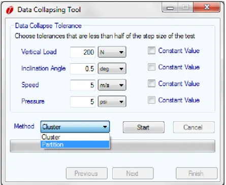
Figure 2.9: Data Collapsing Tool

First the data is sorted into different sets depending on the test conditions. In order to do this the data collapsing tolerances should be set at less than half of the step sizes used in the tire testing. For example if a tire was tested at vertical loads of 100, 200, and 300 lbs the data tolerance should be set to at least less than 50 lbs. This will separate the different test conditions as well as sort out any irregular data. Select the constant value check box for test conditions that are kept constant throughout the test. This will increase the speed of the sorting.

There are two sorting methods availablecluster andpartition. The cluster method works by creating a number of evenly spaced clusters and assigns each data point to the nearest cluster. The sizes of the initial clusters is determined by the variable tolerance. The algorithm then checks all the clusters. If the range of the cluster is too large the cluster is split if it is too small the cluster is deleted. The algorithm continues this process untill all the clusters meet the size crtieria. The partitioning method works by assigning each data point to its own cluster. The algorithm then checks the difference between adjacent clusters if the clusters are too close they are merged. The algorithm continues until the minimum distance between clusters has met the conditions defined by the variable tolerance.

Clicking on the Start button will sort the data. Once this is completed click on the Next

button.

A list of the different sets of data will then be displayed. This is shown in Figure 2.10. The rows of data can be sorted by value by clicking on the column headers.

(29)

the data at the very beginning or end of the test was not removed with the cropping tool it can be removed here. This data will normally be at significantly different speeds or vertical loads than the rest of the data. Also if the data has a relatively low number of samples it most likely was not intended to be tested at those conditions. To remove sets of data just unselect the checkboxes next to that set. Once this is completed click on Next.

Figure 2.10: Sorted Data

Then the discretization range over which the data will be collapsed must be selected. This is shown in Figure 2.11. This determines the quantity and range of the collapsed data points that will be generated. Therefore for pure cornering data the number of steps used for the slip angle should be higher than that for the slip ratio and vice versa for the combined lateral and longitudinal data. For combined data the number of steps used should be approximately equal.

(30)

Figure 2.11: Setting Discretization Range

Clicking on the Collapse Data button will begin the collapsing process. This will compress each set of data points that fall within each discretization step. For each step, the subsequent data points are normalized with respect to their average vertical load. This is demonstrated in the following equations whereFy is normalized with respect to the vertical load. A similar

formulation is used to normalize the other output parameters (i.e. Fx,Mz, etc. . . ).

Fy =

Fz

Fz0

∗Fy0(α0) (2.1)

With the normalized slip angle

α0 = Fz0

Fz

∗α (2.2)

Clicking on the Finish button will close the Data Collapsing Tool and return to the main OptimumT window. A summary of the collapsed tire data will now appear in the data entry area when the tire data is selected in the project tree. The check-box labeled Use Collapsed Data will automatically be checked after the data is collapsed. This checkbox specifies whether the original or collapsed data will be used for graphing and fitting of tire models. This can be seen in Figure 2.12.

(31)

Figure 2.12: Summary of Collapsed Data in the Data Entry Form

The summary of the collapsed data shown in Figure 2.12 allows the user to quickly see the data sets and the conditions of the test. The data can be sorted numerically by clicking on the column headers. The data can also be sorted by the tolerances by selecting the Sort by Tolerance checkbox. The checkboxes in the first column allow the user to exclude or include certain data sets from graphing and tire model fitting. Since the original raw data is still stored in OptimumT the same data can be collapsed multiple times.

2.4 Exporting Data

By selecting the Options-Export button at the top of the raw data entry form the tire data can be exported to an OptimumT Raw Data File or a CSV file. After the desired format is selected a dialog box will appear. Clicking on the Yes button will export the cropped and collapsed tire data while clicking on the No button will export the raw tire data.

(32)

Chapter 3 Tire Models

Currently, seven tire models are implemented in OptimumT:

• Fiala Model

• Brush Model

• Harty Model

• Pacejka Magic Formula ’96 Model

• Pacejka Magic Formula 2002 Model

• Pacejka Magic Formula 2002 Model with Inflation Pressure effects

• Pacejka Magic Formula 2006 Model

The coefficients of these tire models can be manually inputted or imported from an Opti-mumT Native File. OptiOpti-mumT can also fit these models to raw tire data. More specific information regarding the tire models is included in the section 8.

3.1 Manually Input Model

If the tire model coefficients have already been determined, they can be manually inputted into OptimumT. First select the New Tire Model button at the top of the project tree. Then choose the type of tire model you would like to add to the project. This tire model will be added to the project tree. Right clicking on the tire model allows the user to rename, delete, or copy the model as well as many other functions. The model coefficients can now be entered into the model input form, which appears in the data entry area when the model is clicked on. An example of this form is shown in Figure 3.1. For coefficients that have

(33)

units the units can be specified in the dropdown boxes to the right of the value. The small plus and minus buttons also to the right of the values allow the user to adjust the model. This feature is covered in detail in section 3.6.

(34)

(35)

3.2 Import and Export Models

Before a tire model is imported into OptimumT the appropriate tire model needs to be added to the project. This is done by clicking on theNew Tire Model button at the top of the tire project tree. Once the tire model is added clicking on it will display its coefficients in the data entry area. Since it is a new model all of the coefficients will be zero. At the top of the data entry area click on Options-Import as shown in Figure 3.2. Tire model coefficients can then be imported from an OptimumT Native file or from a TIR, or similar, file. Note that when you import a model, OptimumT will overwrite the data contained in the model input form.

Figure 3.2: Import Tire Model

Tire models can also be exported from OptimumT by clicking on the desired tire model in the project tree. Then, at the top of the data entry area, click onOptions-Export and select the file format you prefer. You can export to OptimumT Native files, Excel, Lookup tables and into text-based files, such as TIR files. You also have the option of copying the tire model to the clip board for use with the addin (it will be in an encoded text format).

(36)

Figure 3.3: Export Tire Model

3.2.1 Export Templates

When exporting to a text-based format format, like a TIR file, OptimumT uses export templates. You can edit the export templates in the template manager. When creating a new template, it is recommended that you start with an existing template and modify it. (If you start from a Predefined template, you will need to clone it first because these are read-only). When OptimumT reads a template, it looks for parameter fields in the format

#PARAM#DEFAULT-VALUE#. Note that there are a total of three#symbols for each parameter.

PARAMdenotes the name of the parameter, DEFAULT-VALUEdenotes the default value for this parameter if it is not found in the tire model. If there are parameters specified in the export template that are not in the tire model, the user will be asked to specify them in a dialog when exporting a model. The default value will be used if the user does not specify a different value when exporting. The model description and coordinate system can be exported using the tags#DESC# and #COORDSYS# respectively.

When exporting models using templates be aware that the simulation program you intend to use the model with may require the model in a specific coordinate system. Tir and similar files do not contain coordinate system information so the coordinate system must be modified within OptimumT before exporting. In the case of the MF5.2 and P96 templates, which have been designed for use in RaceSim, you can not export using the SAE coordinate system. It is recommended that you export using the Iso coordinate system for these models. OptimumT also offers the ability to export lookup tables for simulation programs that do not directly import model coefficients or equations. For more details on how to use this feature of OptimumT see section 6.5.

(37)

3.2.2 Excel Export Templates

OptimumT can also export to Microsoft Excel using export templates similar to those ex-plained in the previous section 3.4. An Excel template is a regular Excel worksheet with cells that contain text that can be recognised by OptimumT. When OptimumT reads an Ex-cel template it looks for parameter fields in the format#PARAM#where PARAM is the name of the coefficient to be exported, eg. pCy1 as shown in Figure 3.4. The model description and coordinate system can be exported using the tags#DESC# and #COORDSYS# respectively (Note OptimumT will only search the first worksheet of an Excel template for the parameter fields). Once the template has been created the file should be copied and pasted into the application data folder using the template manager or saved in the application data folder: Windows Vista and Windows 7:

C:\Users\UserName\AppData\Roaming\OptimumT\ExcelTemplates

Windows XP:

(38)

Figure 3.4: Example Excel Export Template

3.3 Fitting Models to Raw Data

Before fitting a tire model to the raw data the data should be properly cropped and col-lapsed. This will make the fitting more accurate and significantly quicker. Also make sure that the Use Collapsed Data option is selected for the tire data that will be used. This can be found at the top of the Collapse Data section in the tire data input area. The following sections demonstrate how to fit a tire model. This example will use pure lateral and com-bined longitudinal and lateral data to create a complete tire model. Depending on the data available and the goal of the model fitting the order in which the models are fit can vary. More information about the order the models should be fit is included in section 3.4.

(39)

3.3.1 Pure Lateral Model

Fitting of the cornering data to the model lateral force coefficients is generally done first. To begin select the tire data to be modeled in the project tree. Go to the last section of the data entry area, labeled Model Fitting. This is shown in Figure 3.5. In the drop down box select the type of tire model to be fitted. Once you have selected the type of model to be used click the Fit Model button. This will open the Model Fitting Tool as can be seen in Figure 3.6.

Figure 3.5: Selecting the Tire Model to be Fit

Specify Coefficients to be Calculated

In theModel Fitting Selectionwindow the coefficients to be fit are selected. The coefficients that the error calculation is based on are also selected by choosing the Fit and Calculate Error option in the dropdown boxes. For this case you would selectFit and Calculate Error

in the drop down box labeled Fy Pure as is shown in Figure 3.6. Fit and Calculate Error

must always be selected for at least one of the sets of coefficients. At the bottom of this window the coordinate system of the model can be selected. To proceed click the Next button.

(40)

Figure 3.6: Model Fitting Selection

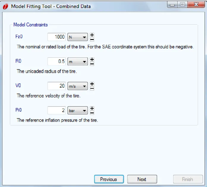
Model Constraints

Now the model constraints must be set. The constraints required vary depending on what type of model is being fit. For the Pacejka models the constraints include the nominal (rated) tire load, Fz0, the unloaded tire radius, R0, the reference velocity, V0, and the reference

pressure,P0. Typically the nominal load is set to the largest or second largest load that the

tire was tested at, the reference velocity is set to the test velocity, and the reference pressure is set to the highest inflation pressure the tire was tested at. More information regarding these parameters is included in section 8.

(41)

Figure 3.7: Model Constraints

Define the Coefficient Boundary

Now theCoefficient Boundaryto be used in the fitting must be set. The coefficient boundary allows the solver to begin fitting the model in a restricted, more accurate range of values for the coefficients. However, the solver is not necessarily restricted to the range of coefficients set by the boundaries. In Figure 3.8 the Coefficient Boundary window is shown. ACoefficient Boundary is chosen by selecting it from the list. Click on Next to proceed.

(42)

Figure 3.8: Coefficient Boundary

Coefficient boundaries can easily be created or edited by clicking on the New Boundary and

Edit Boundary buttons to the right. However the coefficients in thePredefined Folder cannot be modified. If they are edited, the edited version will be saved outside of the Predefined

folder and the original version will stay unchanged. When these buttons are clicked the

Coefficient Boundary Editor window will open as shown in Figure 3.9. This window allows the boundaries for each coefficient to be changed. If the Hard Boundary check boxes are selected the solver will be restricted to finding a solution within this range of coefficients. Save the new or edited boundary by typing in a name at the top of the window and clicking on save. Now you can close this window and the new boundary will be available for selection in the Coefficient Boundary window.

(43)

Figure 3.9: Coefficient Boundary Editor

Weighting Functions

(44)

boundary selection dialog (Figure 3.8). You can also create a new weighting function or edit an existing one in this dialog. If you have selected a weighting function and wish to remove this selection, click the Clear Selection button.

Figure 3.10: The weighting function editor

Figure 3.10 shows the weighting function editor. It is accessible by clicking either the New Weighting or Edit Weighting button. At the very top of the dialog, you can save or load a weighting function. On the left side, you can select the Weighting Pages which define a part of a weighting function. There is no limit to the number of weighting pages that you can add (though there is a practical limit of 60, as it is not possible to define more than 60 non-redundant weighting pages). Each weighting page has one independent variable one ore more dependent variables. If you want to make the solver treat the error of the FxPure fit with more "importance" at high slip ratios, you would define the independent variable to be slip ratio (SR) and the dependent variable to be FxPure. A given pair of independent and dependent variables cannot be defined twice within the same weighting function. You will receive an error if you try to do this.

Once the independent and dependent variables have been selected for a weighting page, the values of the weighting function can be entered. The function is defined as a table. OptimumT will do a linear interpolation between the entries in the table. The Data Value

column indicates the values of the independent variable, and the Weight column defines the weight. Typically the values in the weight column will be between 0 and 1.

(45)

Solver Parameters and Error Evaluation

Next the Population and Iterations needs to be set. These parameters are used by the solver and are not related to the tire models. The Population is the number of initial vales that the solver will distribute between the coefficient boundaries. Therefore if the coefficient boundaries are well defined the population can be less and vice versa. Iterations are the number of steps the solver will take when fitting the model. With a more complex model a larger number of iterations is required. The window that these parameters are set is shown in Figure 3.11.

(46)

at each step. This can help the solver converge towards a global minimum slightly faster. Statistically, the variation is applied equally in both direction, so this technique does not bias the results.

The Error Evaluation can now be selected. This determines what type of error criteria is used when fitting the model. The four types of error criteria included in OptimumT are described below. In the equations Model represents the value found by the model fitter and

Data represents the value of the actual raw data.

• Least Squares Error:

Error = q

P

(M odel−Data)2 P_|Data|

• Normalized Least Squares Error:

Error = r PM odel−Data Data 2 #of datapoints • Total Error: Error = P_{|M odel}₋_Data| P_|Data|

• Normalized Total Error:

Error= P M odel−Data Data #of datapoints

Typically the Least Squares Error criteria will result in the best overall model fit. However depending on the variance and testing conditions of the raw data some of the other error criteria may produce a better fit. For example when fitting an aligning torque model Total Error will often produce slightly better results. The Normalized Error criteria gives equal weight to all of the data points. Therefore it will improve the model fitting at lower loads. In the case that a weighting function is used, the error evaluation is modified to be the following. The weightin is denoted as wi and is evaluated for each data point separately.

• Least Squares Error:

Error = q

P

wi(M odel−Data)2

P_|Data|

• Normalized Least Squares Error:

Error= r P wi _{M odel}₋_Data Data 2 #of datapoints

(47)

• Total Error:

Error = P

wi|M odel−Data|

P_|Data|

• Normalized Total Error:

Error= P wi M odel−Data Data #of datapoints

Model Fitting

Now OptimumT is ready to fit the tire model. However, if something is incorrect or the user would like to change some of the settings the Previous button can be used to go back to the previous windows. Alternatively, the Model Fitting Tool window can be closed and the model fitting restarted.

Clicking on the Summary button allows the user to check to make sure all of the solver settings are correct. It will show the model being fit, the raw data to be used, the error calculation method, the coefficient boundary, and the solver parameters selected. To return to the Model Fitting Tool window just close the model summary. Once the model fitting is finished this information will be automatically transferred into OptimumT and will be stored with the associated tire model in the models data entry form.

Clicking on the Start button in the upper right corner of the window will start the solver. Figure 3.12 shows this window after a fitting has been completed. The graph shows the convergence of the solution and the textbox shows the current error as the model is fitted. When the final solution is found click on the Finish button to return to the main screen of OptimumT.

(48)

Figure 3.12: Model Fitting Convergence and Error

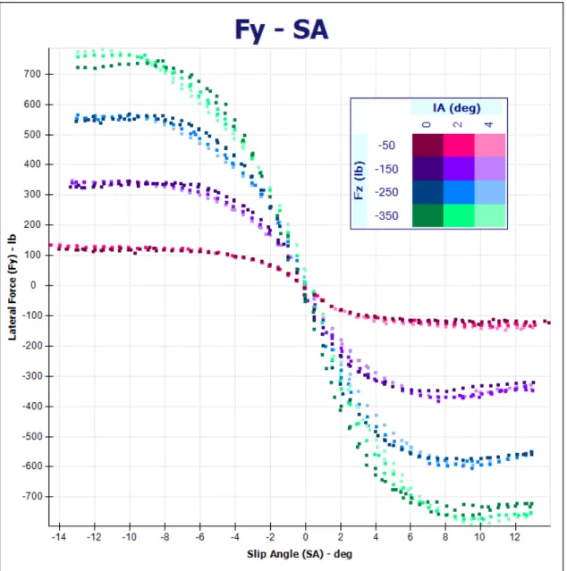
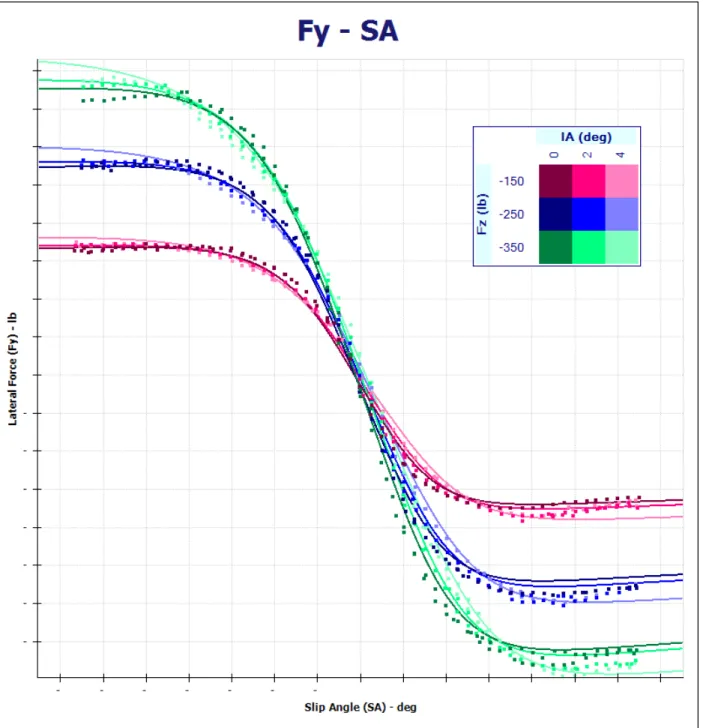
The newly created tire model should now appear in the project tree. This model can now be graphed by selecting the check box next to it (Graphing is covered in Chapter 6). It should be compared to the raw data to ensure accuracy. Lateral force as a function of the slip angle at the tested inclination angles should be graphed and compared to the raw data as shown in Figure 3.13. Also the lateral force as a function of the normal load, Fz, for several slip angles should be graphed as in Figure 3.14. The graphs should be checked for accuracy by comparing them with the raw data. The model should also be checked to ensure the curves are well behaved outside of the measurement area. This is especially important if the tire models are going to be used for simulation. Refer to section 3.6 for information on adjusting the tire model.

(49)

(50)

Figure 3.14: Lateral Force vs. Normal Load at Different Slip Angles

3.3.2 Aligning Torque Model

Fitting the aligning torque model is very similar to the lateral force model. However, there are a few small differences since this model will be combined with the lateral force model. First select the tire data used to fit the lateral force model. In the Model Fitting section

(51)

select the same type of tire model as was used for the lateral force model and click on the

Fit Model button. This will open a different window than before since another tire model already exists in this project. Figure 3.15 shows the Advanced Fitting Options window. In this window coefficients that were already determined in previously created models can be fixed for the current fitting. So for this example you would set the Fy Pure category to the previously created tire model. In later sections you will see that you can set multiple sets of coefficients and also include model scaling factors. Once the correct coefficients are selected click on the Done button.

Figure 3.15: Advanced Fitting Options

Now theModel Fitting Selectionwindow that was used to fit the previous models will open. For this case Calculate and Fit Error in the drop down box labeled Mz Pure would be selected. As can be seen in Figure 3.16 the dropdown box corresponding to Fy Pure is disabled because the coefficients for this model were fixed in the previous step. The rest of the tire model can now be created in the same way as the lateral force model. When finished a new tire model will be created that contains both the pure lateral force and the aligning torque coefficients.

The aligning torque model could also have been created at the same time as the pure lateral force model, but for demonstration purposes was done separately. This would of have been achieved by selecting Fit or Fit and Calculate Error for both Fy Pure and Mz Pure when the coefficients to be fit were specified. The aligning torque as a function of the slip angle should be graphed with the tire data to check the accuracy of the model. An example of this is shown in Figure 3.17.

(52)

(53)

Figure 3.17: Aligning Torque vs. Slip Angle at Different Inclination Angles

3.3.3 Model Scaling Factors

In order to combine the data from a pure cornering test and a combined lateral and longi-tudinal test it will often be required to use a scaling factor. It will adjust the pure lateral force model created from the cornering data to match the combined lateral and longitudinal data at zero slip ratio.

(54)

combined data is the clusters of points at approximately 0, 3, and 6 degrees of slip angle. These points represent the force at zero slip ratio. This discrepancy is an effect of the pure cornering test being performed at a constant slip ratio and varying slip angle, while the combined test is performed at a constant slip angle with a varying slip ratio. These tests are also often performed at different speeds. Additionally, the tire will experience different heat cycling in these tests and therefore different results would be produced.

(55)

Therefore to remedy this problem a scaling factor will be created and applied to the previ-ously created models. To create a scaling factor click on the New Scaling Factor button in the upper right corner of the project tree area. Figure 3.16 shows this button, circled in red. Scaling factors can only be created for the Pacejka models. Similarly to the tire data and models, the scaling factor can be deleted, copied, or renamed by right clicking on it in the project tree.

In Figure 3.19 a previously added scaling factor can be seen in the project tree. The scaling factor can be applied to a tire model by dragging and dropping it onto the tire model or by right clicking on the tire model and choosing Add Scaling Factor. The small red "S" that appears on the selected tire model indicates that a scaling factor has been applied to the model. The scaling factor applied to a tire model can be removed or viewed by right clicking on the tire model.

(56)

Figure 3.19: New Scaling Factor

When a scaling factor is selected in the project tree its coefficients will appear in the data entry area as can also be seen in Figure 3.19. A description of these coefficients appears in Table 8.9. The coefficients can be modified manually or by double clicking on the "+" or "-".

(57)

This will increase or decrease the value of the scaling factor by 10%. If the scaling factor is applied to a graphed model holding down on these buttons will show a preview of the change (For more information on adjusting models refer to section 3.6). Decreasing the peak lateral friction coefficient, λµy, will decrease the lateral force of the model. Figure 3.20 shows the lateral force of the model and data shown in Figure 3.18.

(58)

are tested on are typically different than those they are to be used on. For more information regarding the scaling coefficients and their effect on the models please refer to the section 8.9.

3.3.4 Pure and Combined Longitudinal Model

Now that the previously created model is properly scaled a pure longitudinal and combined longitudinal model can be created. This process will be similar to the previous models but both models will be created simultaneously. They will be created at the same time because the combined lateral and longitudinal tire data is collected at various slip angles. Thus the tire data is representative of pure and combined longitudinal force.

First, the combined data to be used should be imported and properly collapsed (These operations are covered in section 2). Then select the combined lateral and longitudinal tire data in the project tree. In the Model Fitting section select the appropriate tire model and click on the Fit Model button. This will open the Advanced Fitting Options Window. Set the dropdown boxes corresponding to Fy Pure and Mz Pure to the appropriate tire model to fix these coefficients. Click Done once this is completed.

The Model Fitting Selection window will now open. For this case you would select Fit in the Fx Pure drop down box and Fit and Calculate Error in the Fx Combined drop down box as shown in Figure 3.21. You can also calculate the combined error for both models by selecting Fit and Calculate Error for both models. Fit and Calculate Error must be selected for at least one of the models. The rest of the tire model can now be created in the same way as the lateral force model. When finished a new tire model will be created that contains both the pure and combined longitudinal force coefficients.

(59)

Figure 3.21: Fitting Multiple Models Simultaneously

This model should be checked by graphing the longitudinal force as a function of the slip ratio and as a function of the normal load, Fz. Examples of these graphs are shown in Figure 3.22 and Figure 3.23. You should check that the model curves correlate well to the tire data and are well behaved outside of the measurement area especially if the tire model is going to be used for simulation. If the models need to be adjusted please refer to section 3.6.

(60)

(61)

Figure 3.23: Longitudinal Force vs. Normal Load at Different Slip Ratios

(62)

when the model is fit. This is the case because the model will be based on the unscaled Fy Pure coefficients. This is done by selecting the appropriate scaling factor in the Advanced Fitting Options as is shown in Figure 3.24. As can also be seen in the figure all of the previously determined coefficients are set to the appropriate tire model.

Figure 3.24: Fitting with a Scaling Factor

A friction ellipse can now be plotted to ensure the accuracy of the combined lateral and longitudinal models. A graph of a friction ellipse is shown in Figure 3.25. If these models are to be used for simulation it is very important to check that the model curves are well behaved outside of the measurement area.

(63)

Figure 3.25: Friction Ellipse

3.3.6 Additional Models

Additional tire properties can also be fitted to the Pacejka models. These include combined models of aligning torque, rolling resistance, and overturning moment. Table 3.1 summarizes all of the models that can be fit to Pacejka coefficients in OptimumT. It also shows what models are required before creating a new model. The required models can either be fixed prior to or fit concurrently with the new model. These models are fit in the same way as the

(64)

Table 3.1 displays the separate sets of coefficients that are available in the Pacejka models. Only combined, pure, rolling resistance and overturning models can be fit with the Pacejka models. The overturning moment and rolling resistance models are not available in the Pacejka ’96 model.

Model Requires

Fx Pure Longitudinal Force

Fx Comb Combined Longitudinal Force Fx Pure, Fy Pure Fy Pure Lateral Force

Fy Comb Combined Lateral Force Fx Pure, Fy Pure Mx Pure Overturning Moment Not Available

Mx Comb Combined Overturning Moment Fx Pure, Fx Comb (not available in ’96) My Pure Rolling Resistance Not Available

My Comb Combined Rolling Resistance Fy Pure, Fy Comb (not available in ’96) Mz Pure Aligning Torque Fy Pure

Mz Comb Combined Aligning Torque Fx Comb, Fy Comb, Mz Pure

Table 3.1: Pacejka Models (Mx Comb and My Comb are not available in the Pacejka ’96 model)

3.4 Model Fitting Order

The order in which the models are fit can vary depending on the tire data available and the goals of the project. However, since some of the models are dependent on each other there are some restrictions on the order. Table 3.1, above, shows what models are required before other models can be fit. This is also displayed in the Model Fitting Selection window in OptimumT. These requirements, which will vary depending on the type of model being fit, can be seen to the right of the dropdown boxes in Figure 3.26.

(65)

Figure 3.26: Model Fitting Requirements

The two most common model fitting sequences will be described in Table 3.2 and Table 3.3. The first sequence uses pure lateral and combined data like the model fitting example in the previous sections. The second sequence uses pure lateral, pure longitudinal and combined data. Under Coefficients to be Fixed the "Fix" indicates that these coefficients should be selected in the Advanced Fitting Options window. Under Coefficients to be Fit the "FE" indicates that these coefficients should be set to Fit and Calculate Error and the "Fit" indicates that these coefficients should be set toFit in theModel Fitting Selection window.

(66)

Model Fitting with Pure Lateral and Combined Data

Step Data Used

Coefficients to be Fixed Coefficients to be Fit Pure Combined Pure Combined Fx Fy Mz Fx Fy Mz Fx Fy Mz Fx Fy Mz

1 Pure Lat. Fe

2 Pure Lat. Fix Fe

5 Combined. Fix Fix Fit Fe

4 Combined. Fix Fix Fix Fix Fe

5 Combined. Fix Fix Fix Fix Fix Fe

Table 3.2: Model Fitting Order with Pure Lateral and Combined Data

Model Fitting with Pure Lateral, Pure Longitudinal and Combined Data

Step Data Used

Coefficients to be Fixed Coefficients to be Fit Pure Combined Pure Combined Fx Fy Mz Fx Fy Mz Fx Fy Mz Fx Fy Mz

1 Pure Lat. Fe

2 Pure Lat. Fix Fe

5 Combined. Fix Fix Fit Fe

4 Combined. Fix Fix Fix 5 Combined. Fix Fix Fix Fix 6 Combined. Fix Fix Fix Fix Fix

Table 3.3: Model Fitting Order with Pure Lateral, Pure Longitudinal and Combined Data

3.5 Model Coefficient Form

After a model is fit the coefficients corresponding to it can be accessed by clicking on the model in the tire project tree. This will display the model coefficient form in the data entry area as shown in Figure 3.27. This form includes the model coefficients, a description box, and the option to change the name displayed in the legend for the model. In this form the model coefficients can be modified by the user. This will be covered in detail in the next section.

(67)

Figure 3.27: Model Coefficient Form

After a model is fit information regarding the model fitting will be directly imported into the description box as can be seen in Figure The information included in the description box is the final error of the fitting, the model that was fit, the data file used, the coefficients fit, the error evaluation method, the coefficient boundary, and the solver parameters.

3.6 Adjusting Models

Once the model is created and graphed against the raw data you might want to adjust it to improve its accuracy in a certain region or improve its behavior beyond the measurement area. This can be done easily in OptimumT.

(68)

next to the coefficient 1 . If the model is shown on a graph (see chapter 6 for information about graphing), holding down the "+" or "-" button will show a preview of the model with the coefficient modified by 10%. An example of this is shown in Figure 3.28. In this figure the "+" button of thepDy1 coefficient is being held down. As can be seen in Figure 3.28 this change has a large effect on the graph. Changing other coefficients will have a much different effect on the curve both in terms of its magnitude and shape. The coefficients can also be adjusted manually by changing the values in the boxes. When applied to a tire model the coefficients of a scaling factor can be adjusted in the same way.

Figure 3.28: Model Adjustment Preview Feature

(69)

Figure 3.29: Creating a boundary from an existing model.

Figure 3.30: To save the boundary created from a model, specify the name to save it as in this dialog.

3.7 Creating Coefficient Boundaries From an Existing

Model

You can create a boundary from an existing model. When doing this, you specify the half-width of the boundary. In the model coefficient form, click on Options then Create Boundary From Model to arrive at the range specification (shown in Figure 3.29). Enter the desired range and click the check-mark button. The minimum for each coefficient is created by reducing the the coefficient value by the user specified percentage, and the maximum is created by increasing the the value by the same amount. For example, if one of the coefficients of the model has a value or 1.00 and you specify a boundary range of 10%, the minimum will be 0.90 and the maximum will be 1.10.

Once you have clicked the check-mark button to create the boundary, you will be presented with the dialog shown in Figure 3.30. Enter the name to save the boundary as and choose a folder to put the boundary in.

(70)

Chapter 4 Graphing

The OptimumT plotting tool is a powerful feature that allows users to create nearly any type of tire graph that they please. Two different types of graphs can be created in OptimumT. One is astandard graphwhich allows plotting of any quantity against any other quantity in either two- or three-dimensions. The other is areport graphwhich shows measured quantities versus sample number. It is only capable of plotting raw data.

4.1 Standard Graphs

Standard graphs can display raw data and tire models. The data or model to be graphed can be specified by selecting the checkbox next to the desired items in the project tree. A new standard graph can be added to a worksheet in multiple ways. Right clicking on the worksheet or worksheet tabs and selecting Add Graph, selecting Add Graph To Worksheet

from the Worksheet menu on the main toolbar or by clicking on the Add Graph button in the toolbar next to the Save button. Up to four graphs can be placed on a single worksheet. When a graph is added to the worksheet the graph setup form will appear in the data entry area. To show the graph setup form when the data entry area is showing another form, click on the graph. You must specify six graph inputs and two or three graph outputs to create a graph. These will be further discussed in the following sections.

4.1.1 Types of Standard Graphs

There are three types of standard graphs. Single direction line graphs, crossed line graphs and surface graphs. You can select the type of graph by choosing the appropriate option in the list of radio buttons near the bottom of the data entry form.

(71)

Single Direction Line Graphs

An example of a single direction line graph is shown in Figure 4.1. When plotting models using this type of graph, lines are generated based on the first of the graph inputs. For example, if the first graph input (labeled as Indep. Variable) is slip angle, lines will be generated by varying the slip angle while keeping all the other graph inputs constant.

Figure 4.1: Single Direction Line Graph

(72)

input while holding all others constant. The second set of lines is generated by varying the second graph input while holding all the others constant. For example, if the first graph input (labeledFirst Indep.) is set as slip angle and the second input (labeledSecond Indep.) is set as slip ratio, then one set of lines will be generated with constant slip ratio and varying slip angle and another set of lines will be generated with constant slip angle and varying slip ratio. This type of graph is useful when creating a friction ellipse where you want lines of constant slip angle and lines of constant slip ratio.

Figure 4.2: Crossed Line Graph

Surface Graphs

An example of a surface graph is shown in Figure 4.3. Surface graphs are only available when a third graph output is selected in the Depth Axis drop down box. Surfaces are generated

(73)

in the same way that crossed line plots are generated, but the area between the lines is filled to generate the surface.

Figure 4.3: Surface Graph

4.1.2 Setting up a Standard Graph

For OptimumT to generate a graph all six possible steady state tire conditions must be specified. These graph inputs are:

(74)

• Inclination angle, γ • Velocity, V

• Inflation pressure, P

In addition to the six graph inputs, the two graph outputs, the Horizontal Axis and Vertical Axis must be set to create a graph. If you are making a 3D graph a third output, theDepth Axis, must also be specified. Essentially, the OptimumT plotting tool is evaluating a tire model or searching through the tire data for the three axes as follows:

X =f1(α, κ, Fz, γ, V, P)

Y =f2(α, κ, Fz, γ, V, P)

Z =f3(α, κ, Fz, γ, V, P)

4.1.3 Graph Outputs

The graph outputs specify what quantity and data range that each graph axis should repre-sent. The graph output dialog is shown in Figure 4.4. In this dialog the graph output to be used for each axis can be chosen. The unit displayed and the axis scaling can also be chosen. If the Auto Scale check box is selected, the scaling will adjust according to the data shown on the graph. The Auto Scale is unchecked then minimum and maximum value for the axis can be entered. Selecting Hide Axis Values will remove the numeric values from the graph axis.

Figure 4.4: Graph Output Dialog

Currently OptimumT includes over 30 outputs that can be graphed. These outputs as well as their associated unit types are displayed in Table 4.1. The unit types are displayed because

(75)

OptimumT allows the user to select between many different units. For more information about the available units in OptimumT please refer to section 8.3.

Graph Outputs

Basic Unit Type

Inclination Angle (IA) angle Slip Angle (SA) angle Slip Ratio (SR) ratio Speed (V) velocity Pressure (P) pressure Loaded Radius (RL) length

Force / Moment Unit Type

Longitudinal Force (Fx) force Lateral Force (Fy) force Normal Load (Fz) force Overturning Moment (Mx) moment

Rolling Resistance (My) moment Aligning Torque (Mz) moment

Derivatives Unit Type

Cornering Stiffness force / angle Inst. Cornering Stiffness force / ratio Slip Stiffness force / angle Inst. Slip Stiffness force / ratio Camber Stiffness force / angle Inst. Camber Stiffness force / angle Lateral Load Sensitivity ratio Longitudinal Load Sensitivity ratio Aligning Moment Load Sensitivity length Overturning Moment Load Sensitivity length Rolling Resistance Load Sensitivity length

Normalized Unit Type

Normalized Longitudinal Force ratio Normalized Lateral Force ratio Normalized Inst. Cornering Stiffness 1 / angle

Normalized Inst. Slip Stiffness ratio Normalized Inst. Camber Stiffness 1 / angle

(76)

Coefficient of Friction Unit Type

Lateral Coefficient of Friction ratio Longitudinal Coefficient of Friction ratio

Moment Arm Unit Type

Pneumatic Trail length Pneumatic Scrub Radius length

Peak Unit Type

Slip Angle at Peak Fy (negative) angle Slip Angle at Peak Fy (positive) angle Slip Ratio at Peak Fx (negative) ratio Slip Ratio at Peak Fx (positive) ratio Peak Lateral Force (negative) force Peak Lateral Force (positive) force Peak Longitudinal Force (negative) force Peak Longitudinal Force (positive) force

Offset Unit Type

Fx Offset (Fx @ SR = 0) force Fy Offset (Fy @ SA = 0) force

Table 4.1: Graph Outputs

4.1.4 Graph Inputs

The graph inputs can be fixed values, constant sweeps orcustom sweeps. The graph inputs are specified by clicking on the box next to one of the six graph inputs. A dialog box similar to that shown in Figure 4.5 will appear. The first item to be chosen is the variable for the graph input. This is chosen in the first dropdown box of the dialog. As can be seen in Figure 4.5 "Slip Angle" is currently selected as the first independent. As previously mentioned, all six inputs must be present.

For a Single Line graph the first graph input, labeled Indep. Variable, will be the quantity used to generate the graph lines. For a Crossed Line or Surface graph the first two graph inputs, labeled First Indep. and Second Indep., will be the quantities used to generate the graph lines. The rest of the graph inputs, labeled Sweep, allow the plotting of multiple lines

(77)

depending on the other tire conditions. For the first two of these, the option of changing the color of the graphed lines according to these inputs is available (see section 4.1.8 for more information).

The second dropdown box in this dialog allows the user to specify the type of sweep to be graphed. For each input in the graph input dialog three different types of sweeps can be chosen. The three sweep types available are: Fixed Value, Constant Step Sweep, and

Custom Sweep. For the independent variables either the Constant Step Sweep or Custom Sweep should be used. For the sweep variables any of the sweep types can be used.

Figure 4.5: Graph Input Dialog

Fixed Value Graph Inputs

As the name suggests, fixed value graph inputs hold a particular variable constant when generating the graph. In the example shown in Figure 4.6, Fixed is selected in the second drop down box. Therefore the inclination angle is being held at a constant 2 degrees. In the fixed value dialog, there is also a box for data tolerance. This value tells OptimumT what tolerance to use when searching raw data. Since there will always be some noise in the raw data, OptimumT needs to know how far from the nominal value it should consider to be "close enough" to include in the plot.

(78)

Figure 4.6: Fixed Value Dialog

Constant Step Sweep Graph Inputs

Constant step sweep graph inputs generate a set of evenly spaced points between a minimum and a maximum value. The constant sweep dialog is shown in Figure 4.7. A minimum and a maximum value for the sweep as well as the number of steps needs to be entered into the dialog. Constant sweep graph inputs do not have data tolerances as fixed graph inputs do. All data that falls within the specified range is used.

(79)

Custom Sweep Graph Inputs

A custom sweep graph input allows you to specify a number of arbitrary values. Figure 4.8 shows the custom sweep dialog. You can specify any number of values by typing them into the table. Additional rows can be added by clicking on the green "+" and rows can be removed by clicking on the red "-" above the input list. Like the fixed value graph input, custom sweep graph inputs have data tolerances.

(80)

4.1.5 Plotting Raw Data

Initially when raw data is imported and graphed in OptimumT all of the data will be plotted regardless of the graph input parameters. ThisPlot all Datafeature allows the user to quickly view data to ensure that it is the correct data and that it was imported successfully. If the user would like to graph data at certain conditions specified by the graph inputs, this feature needs to be unselected.

When thePlot all Dataoption is unselected, OptimumT will search for raw data points that correspond to all six of the graph inputs. Points matching the six conditions will be plotted on the graph.

There are three different ways to unselect thePlot All Data. The first one is by right clicking on the raw data in the project tree and selecting Remove "Plot All Data" In All Graphs. This is shown in Figure 4.9. This will disable the feature for the selected data set in all of the graphs.

Figure 4.9: Plot All Data Option in Project Tree

Help File Version

Help File

Version 1.0.14

By

engineering@optimumg.com

www.optimumg.com

Welcome

Feedback

Features Coming Soon

Contents

Introduction

Installation Requirements

Hardware Requirements

Processor

Memory

Storage

Display Adapter

Display Unit

Other

Software Requirements

Operating System

Required Software Components

Other

License

Moving License

License Viewer

Chapter 1

Screen Layout

1.1

Tire Project Tree

Raw Data

Tire Models

Scaling Factors

1.2

Data Entry Form

1.3

Worksheets

Chapter 2

Raw Tire Data

2.1

Importing Data

2.2

Data Cropping

2.2.1

Data Cropping Templates

2.3

Data Collapsing

2.4

Exporting Data

Chapter 3

Tire Models

3.1

Manually Input Model

3.2

Import and Export Models

3.2.1

Export Templates

3.2.2

Excel Export Templates

3.3

Fitting Models to Raw Data

3.3.1

Pure Lateral Model

Specify Coefficients to be Calculated

Model Constraints

Define the Coefficient Boundary

Weighting Functions

Solver Parameters and Error Evaluation

Model Fitting

3.3.2

Aligning Torque Model

3.3.3

Model Scaling Factors

3.3.4

Pure and Combined Longitudinal Model

3.3.6

Additional Models

3.4

Model Fitting Order

3.5