ECONOMIC GROWTH CENTER
YALE UNIVERSITY
P.O. Box 208629
New Haven, CT 06520-8269
http://www.econ.yale.edu/~egcenter/
CENTER DISCUSSION PAPER NO. 944
Selection and Comparative Advantage
in Technology Adoption
Tavneet Suri
Massachusetts Institute of Technology
September 2006
Notes: Center Discussion Papers are preliminary materials circulated to stimulate discussions and critical comments.
MIT Sloan, email: [email protected]. I am extremely grateful to Michael Boozer for countless hours of discussion on this project. I would also like to thank the rest of my committee, Gustav Ranis, Paul Schultz and Christopher Udry, as well as Robert Evenson, Fabian Lange and seminar audiences at Yale and NEUDC for comments. A special thanks to Thom Jayne and Margaret Beaver at Michigan State University for help with the 1997-2002 rounds of the data. I am sincerely grateful to the Tegemeo Institute and Thom Jayne for including me in the 2004 survey and especially to Tegemeo for their hospitality during the field work in Kenya. I would like to thank James Nyoro, Director of Tegemeo, as well as Tegemeo Research Fellows Miltone Ayieko, Joshua Ariga, Paul Gamba and Milu Muyanga, Senior Research Assistant Frances Karin, and Research Assistants Bridget Ochieng, Mary Bundi, Raphael Gitau, Sam Mburu, Mercy Mutua and Daniel Kariuki and all the field teams for their impressive work through all the rounds of the survey, especially 2004. An additional thanks to Margaret Beaver and Daniel Kariuki for spending immense energy ensuring the data was squeaky clean. The data come from the Tegemeo Agricultural Monitoring and Policy Analysis (TAMPA) Project, between Tegemeo Institute at Egerton University, Kenya and Michigan State University, funded by USAID, April 1996 - June 2005. Any rainfall data used come from the Climate Prediction Center and are part of the USAID/FEWS project - thanks to Tim Love for his repeated help with these data.
This paper can be downloaded without charge from the Social Science Research Network
electronic library at: http://ssrn.com/abstract=933124
An index to papers in the Economic Growth Center Discussion Paper Series is located at:
http://www.econ.yale.edu/~egcenter/research.htm
Selection and Comparative Advantage in Technology Adoption
Tavneet Suri
ABSTRACT
This paper examines a well known empirical puzzle in the literature on technology adoption: despite
the potential of technologies to increase returns dramatically, a significant fraction of households
do not use these technologies. I study the use of hybrid maize and fertilizer in Kenya, where there
are persistent cross-sectional differences in aggregate adoption rates with a large fraction of
households switching in and out of adoption. By allowing for selection of farmers into technology
use via comparative advantage differences, I examine whether the yield returns to adopting hybrid
maize vary across farmers. If so, high average returns can coexist with low returns for the marginal
farmer. My findings indicate the existence of two interesting subgroups in the population. A small
group of farmers has potentially high returns from adopting the technologies. Yet, they do not adopt.
This lack of adoption appears to stem from supply and infrastructure constraints, such as the distance
to fertilizer distributors. In addition, a larger group of farmers faces very low returns to adopting
hybrid maize, but chooses to adopt. This latter group might benefit substantially from the
development of newer hybrid strains to increase yields. On the whole, the stagnation in hybrid
adoption does not appear to be due to constraints or irrationalities.
Key Words:
Technology, Heterogeneity, Comparative Advantage
JEL Codes:
C33, O12, Q12
1
Introduction
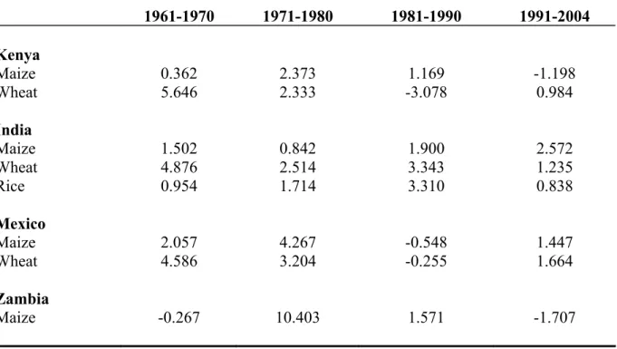
Food security is currently at the forefront of the policy agenda across many Sub-Saharan African economies. Agricultural yields have fallen in the last decade across many of these economies, despite the widespread availability of technologies that increase yields. Governments and policy makers need to understand why yields of agricultural staples are low across parts of Africa in order to …nd ways to enhance food production and incomes. Table 1 shows the falling yields of staple crops over the last decade in Kenya, compared with increasing yields in India and Mexico. These are worrisome trends: it seems as if Kenya has not yet been able to take the same advantage of improvements in agricultural technologies as have India and Mexico during their Green Revolutions.
This paper examines adoption decisions faced by farmers in rural Kenya with respect to agri-cultural technologies, in particular hybrid maize and fertilizer. What agriagri-cultural technologies are households using and are these technologies actually increasing yields for all farmers? Why are some farmers not adopting, even though others in the same community adopt and seem to receive signi…cant yield increases? Understanding how and why households decide what tech-nologies to adopt is crucial for understanding the trends in agricultural yields in Sub-Saharan Africa, where risk and incomplete factor markets are potentially important.
Field trials at experiment stations across Kenya show that hybrid maize and fertilizers can increase yields of maize signi…cantly, increases ranging between 40 and 100% (see Gerhart (1975), Kenya Agricultural Research Institute, KARI (1993), Karanja (1996)). The Fertilizer Use Rec-ommendations Project (FURP) conducted in Kenya in the early 1990’s also shows high returns to these technologies in …eld trials (see Hassan et al (1998)) - results con…rmed in the small sam-ple of Du‡o, Kremer and Robinson (2003). However, aggregate adoption rates of hybrid maize and fertilizer remain far below 100% across Kenya, with large variations in individual adoption status from year to year. This has posed an empirical puzzle: why are aggregate adoption rates low and stagnating when returns to the technologies are so high? The literature has put forth a number of explanations from models of learning and informational barriers, credit constraints, taste preferences to the lack of e¤ective commitment devices (see Du‡o, Kremer and Robinson (2003)).
My approach to these questions of technology adoption is very di¤erent from the standard literature. I examine whether the yield returns to adopting hybrid maize vary across a random sample of maize farmers, such that high average returns to the technologies are accompanied by low returns for the marginal farmer. Allowing heterogeneity in returns to play a role in the adoption decision implies that the knowledge of average returns is not enough to understand the adoption decisions across a sample of farmers. I study the adoption of agricultural technologies in Kenya within a framework of heterogeneous returns where a farmer’s expected bene…ts from the technology are allowed to be correlated with his decision to adopt the technology. I there-fore model technology adoption as a selection process where yields may be heterogeneous and expected bene…ts to the technology may drive adoption decisions in each period. This allows
for household-speci…c heterogeneity in returns and hence controls for selection via comparative advantage di¤erences across households.
I use an extensive panel dataset representative of maize-growing Kenya, covering the period from 1996 to 2004. I helped design and collect the 2004 round of this panel survey. I …rst document the adoption patterns of households over the period 1996 to 2004, for both hybrid maize and fertilizer. I …nd that aggregate adoption over the period is stable over time, even when I look across regions or asset/wealth quintiles. What is striking in my data is that I observe very di¤erent adoption rates across regions and asset quintiles, but these adoption rates are stable over time. What is even more surprising is that at least 30% of my households switch into and out of use of hybrid seed over my sample period.
I then turn towards estimating and testing models with homogeneous returns, as well as models with speci…c forms of unobservable heterogeneity, i.e. household …xed e¤ects models. These serve as a baseline for my later contributions. I look at some empirical tests of these models and in general, such models are rejected in my data. So, I present a more general model of heterogeneous returns and selection. In a methodological contribution, I generalize Chamber-lain’s (1982, 1984) approach to the …xed e¤ects model to accommodate not just heterogeneous intercepts, but also heterogeneous slopes (here, returns to hybrid). Overall, I …nd strong evi-dence of heterogeneity and selection of farmers into the use of technologies. There is evievi-dence of farmers responding to their expected bene…ts by selecting into the use of high yielding varieties. I …nd that even though these agricultural technologies have high average returns, the marginal farmer has low returns and switches easily in and out of adoption when subject to idiosyncratic shocks.
The empirical strategy I use allows me to estimate the distribution of returns in my sample (under certain assumptions). The joint distribution of returns and adoption decisions displays some extremely interesting features. In particular, I observe a small group of farmers with high returns from hybrid seed, yet they choose not to adopt. The lack of adoption for this small set of households appears to stem from supply and infrastructure constraints, such as distance to seed and fertilizer distributors. On the ‡ip side, I also …nd a comparatively large group of households for whom the returns are extremely low, almost zero, yet they adopt hybrid maize. These results point to the need for focused interventions for policy to be cost e¤ective. For the constrained farmers, alleviating their constraints by improving infrastructure and distribution would improve yields dramatically. The unconstrained farmers, however, may bene…t greatly from the development of new hybrid strains.
The rest of this paper is structured as follows. In Section 2, I outline some of the relevant literature, focusing on empirical studies. Section 3 describes the data I use and some background and history of maize cultivation in Kenya. Section 4 discusses models of adoption decisions, focusing on the economics motivating my model of heterogeneous returns. Section 5 discusses the results for the standard household …xed e¤ects model, a test of this model, as well as some evidence for selection and heterogeneity in returns. Section 6 describes estimation of the
heterogeneous returns model and the associated distribution of returns. In Section 7, I cover some robustness checks, in particular the Heckman two-step estimator as well as treatment e¤ects under non-random assignment, i.e. the average treatment e¤ect (ATE), the treatment on the treated (TT), the marginal treatment e¤ect (MTE) and the local average treatment e¤ect (LATE) or IV estimator. Section 8 discusses the implications of my results for households and policy makers in Kenya. I discuss why a framework like mine is needed for a country like Kenya, which has widely varying agronomic conditions. Section 9 concludes.
2
Literature Review
I brie‡y summarize some of the empirical literature on technology adoption2 in developing countries, with a focus on the studies that have been conducted in Sub-Saharan Africa. Gerhart (1975) is the most relevant study for my paper so I discuss his research …rst. He tracks the adoption of hybrid maize in Western Kenya in the late 1960’s and early 1970’s. Gerhart highlights the fast di¤usion of hybrid maize in this region and identi…es constraints to the use of hybrid maize. He …nds that risk is extremely important: if farmers had other means of dealing with risk (such as other drought resistant crops, cash crops or o¤ farm income), then they were far less likely to use hybrid maize. In addition, education of the farmers, credit availability, extension services were all important in determining hybrid use. Finally, farmers who used hybrid maize were also more likely to use other improved farming technologies, such as fertilizer use, manure use, planting in rows, etc.
I split the rest of this review into four main areas, …rst discussing studies that relate to het-erogeneity, then looking at research on learning externalities and credit constraints and ending with the recent experimental research. The seminal empirical paper on new agricultural tech-nology adoption is Griliches (1957)3. He looks at the heterogeneity across local conditions in the adoption speeds of hybrid corn in the Midwestern US. Griliches emphasizes the role of eco-nomic factors like expected pro…ts and scale in determining the variation in di¤usion rates. He also notes how the speed of adoption across geographical space depends on the suppliers of the technology and when the seed was adapted to local conditions. Other researchers have looked at heterogeneity along other dimensions, focusing on describing what forms of heterogeneity drive the decisions of households to adopt new technologies. This covers quite a range of papers: from Schultz (1963) and Weir and Knight (2000), who emphasize the role of education, to the various CIMMYT (The International Wheat and Maize Improvement Center) studies4 that collect data
2
The literature on technology adoption is too vast to review here, excellent reviews can be found in Sunding and Zilberman (2001), Sanders, Shapiro and Ramaswamy (1996), Rogers (1995), and Feder, Just and Zilberman (1985). There is a large theoretical literature, for example, Besley and Case (1993), Banerjee (1992) and Just and Zilberman (1983). For other …elds of economics, Hall (2004) reviews well the social, economic and institutional determinants of di¤usion rates. I do not discuss studies that focus on livestock or land management practices (Mugo et al (2000)), agricultural extension (Evenson and Mwabu (1998)), or property rights (Place and Swallow (2000)).
3
Also see David (2003).
on what underlies adoption decisions across di¤erent parts of Kenya. For example, Makokha et al (2001) look at the determinants of fertilizer and manure use in Kiambu district in Kenya, focusing on measuring soil quality and showing that farmers’perceptions of soil quality are rea-sonably accurate. The main (self-reported) constraints to using fertilizer were high labor costs, high prices of inputs, unavailability of demanded packages and untimely delivery. Ouma et al (2002) look at the adoption of improved seed and fertilizer in Embu District in Kenya where they …nd that gender, agroclimatic zone, manure use, hiring of labor and extension services are signi…cant determinants of adoption. Similarly, Wekesa et al (2003) look at the adoption of the Coast Composite, Pwani 1 and Pwani 4 hybrids and fertilizer in the Coastal Lowlands of Kenya where the non-availability and high cost of seed, unfavorable climatic conditions, perceptions of su¢ cient soil fertility, and lack of money/credit are cited as reasons for low use.
Much of the recent literature on technology adoption has focused on the learning externality, described well by Besley and Case (1993), which relates to the literature on social interactions. Foster and Rosenzweig (1995) look at the adoption of high yielding varieties in post Green Rev-olution India, allowing for learning by doing, learning from others, and costly experimentation. They …nd that farmers with more experienced neighbors are more pro…table than those without. Munshi (2003) looks at the same question and …nds that the impacts are heterogeneous: wheat growers respond strongly to their neighbors’experiences while rice farmers experiment. He …nds greater variations in yields in rice growing areas and notes that rice high yielding varieties, unlike those for wheat, tend to be sensitive to soil characteristics and managerial inputs, which are di¢ cult to observe. Conley and Udry (2003) study the adoption of fertilizer in the small-scale pineapple industry in Ghana. They collect information on farmers’sources of information and …nd evidence of learning, not only from own experiences, but also within information neighbor-hoods. Bandiera and Rasul (2003) look at decisions to plant sun‡ower in the Zambezia province of Mozambique. They …nd that adoption decisions are correlated within networks of family and friends and that this e¤ect is stronger for disadvantaged farmers. Moser and Barrett (2003) look at a high yielding low external input rice production method in Madagascar, analyzing decisions to adopt, expand and disadopt. They …nd seasonal liquidity constraints and learning e¤ects from extension agents and other households to be important.
A hypothesis that is often raised in the literature is that credit constraints explain the lack of adoption. For example, Croppenstedt, Demeke and Meschi (2003) estimate a double hurdle fertilizer adoption model for Ethiopia, using self-reported information on why farmers did not purchase fertilizer. They …nd that credit is a major supply side constraint to adoption. Most of the CIMMYT studies also cover self-reported credit constraints; for example, Salasya et al (1998) look at the role of credit in adoption decisions in Western Kenya.
The …nal strand of literature on Kenya I describe is experimental. There are several impact assessment studies5 and …eld trials at experiment stations which show large increases in yields
see http://www.cimmyt.org/research/economics/map/impact%5Fstudies/impstudea%5Flist/ for all the impact studies done by CIMMYT in East Africa.
5
from using hybrid maize and fertilizer. Other than the work done by the Kenya Agricultural Research Institute on experiment stations, one of the earlier experimental studies was the Fer-tilizer Use Recommendations Project (FURP), conducted across 70 sites in the early 1990’s in conjunction with the Kenya Maize Database Project (MDBP). FURP recorded yields about half of those on experimental stations (KARI (1993)). The focus of these experiments was to understand optimal rates of fertilizer use in comparison to survey data on actual use from the MDBP (see Corbett (1998)). Hassan et al (1998) use these data and …nd that both adoption of hybrid maize and varietal turnover rates are higher (and di¤usion faster) in high potential areas. They blame poor extension services, bad infrastructure and poor seed distribution for the low adoption rates in the marginal areas. Hassan, Murithi and Kamau (1998) combine the data from the surveys and trials and …nd that farmers apply less fertilizer than is optimal, leading to an estimated 30% gap between current and optimal yields.
A more recent example is De Groote et al (2003) who look at an ex-ante impact assessment of the Insect Resistant Maize for Africa (IRMA) project that develops GM maize varieties that are more resistant to stem borers. They estimate the surplus from a shift in supply due to the decreased crop loss (measured experimentally) as a result of introducing this maize variety that is more resistant to stem borers. Estimated crop losses amounted to 13.5% with an estimated value of $80 million. The results imply high returns to such genetic technologies6. Similarly, Du‡o, Kremer and Robinson (2003) run controlled experiments in the …eld to measure returns from fertilizer use. They …nd that the average net rate of return for investing in top-dressing fertilizer is between 28% and 134% for an eight month investment. They study di¤usion and …nd a signi…cant negative impact on neighbors of the program. They …nd that farmers learn via demo trials, distributed kits, but not through announcements of government endorsement. They started the Savings and Fertilizer Initiative (SAFI) as a commitment device for farmers and …nd that farmers take up this program when it is o¤ered at harvest time, but not later, pointing to these farmers being hyperbolic discounters.
3
Survey Data and Maize Cultivation in Kenya
Maize is the main staple in Kenya7, accounting for approximately 3.7 million acres of cropped
land with main season maize production ranging between 2.3 and 2.7 million MT, of which
Karanja, Renkow and Crawford (2003) look at di¤erential impacts across high potential and marginal areas in Kenya, in terms of e¢ ciency and distribution. They …nd that adoption of technologies in high potential areas, relative to those in marginal areas, have large aggregate gains at the expense of poor distributional e¤ects. Sserunkuuma (2002) looks at a partial equilibrium model of adoption of improved maize and fertilizer in Uganda. He uses price elasticities of demand and supply from secondary sources to estimate large consumer gains and large producer losses of a shift in supply due to the adoption of hybrid maize.
6See http://www.cimmyt.org/ABC/InvestIn-InsectResist/htm/InvestIn-InsectResist.htm and Smale and De Groote (2003) for more information on the CIMMYT IRMA and GM projects in Kenya.
7McCann (2005) describes the fascinating history of maize in Africa pointing out how maize not only gives more food per unit of land and labor, but also has the largest set of alternative uses compared to other grains. Nyameino, Kagira and Njukia (2003) cite that about 90% of Kenya’s population depends on maize for income generation.
75% is through small-scale farming. Average maize yields are on the order of 0.8 MT per acre, although there is considerable cross-sectional diversity.
I use data from the Tegemeo Agricultural Monitoring and Policy Analysis (TAMPA) Project (April 1996-June 2005) between Tegemeo Institute at Egerton University, Kenya and Michigan State University8. This is a household level panel survey, representative of rural maize-growing
areas, which are geographically very diverse. Figure 1 shows a map of Kenya with the location of the villages covered.
Di¤erent modules of data were collected in di¤erent years of the survey, with a common core set. I have data for 1997, 1998, 2000, 2002 and 2004. The 1997, 2000 and 2004 surveys are similar, containing detailed agricultural input and output data (plus retrospective data for 1995-1996), household consumption (not complete), income, demographics (individual age, gender, education and health), infrastructure, location, and some basic credit information. The panel sample covers about 1400 households, with an additional 800 households in the 2004 sample. The 1998 survey is similar, but covers only a sub-sample of about 612 households. Kenya was strongly a¤ected by El Nino in 1998 and so the 1998 sample is very di¤erent from other years. The 2002 survey was a short proxy survey, but it collected detailed data on hybrid maize use. I restrict myself mostly to 1997, 2000 and 2004 data.
To motivate my research questions, I outline some trends in my data over the period 1996-2004 on the use of hybrid maize and fertilizer. Figure 2 shows the trends in adoption of hybrid maize for the two seasons, de…ned here as the fraction of maize seed planted that is hybrid. Figure 3 looks at main season adoption patterns by province over the same period. Both Figures 2 and 3 illustrate the stability in aggregate adoption patterns over time and the persistence of cross-sectional di¤erences. An identical pattern is evident if I look across wealth/asset or acreage quintiles. The use of inorganic fertilizer during the main season follows similar trends. Figure 4a shows the trends across provinces in the fraction of households that use inorganic fertilizer for maize production and Figure 4b shows the total value (in constant Kenyan shillings) of inorganic fertilizer used, by province. There is a lot more variation over time in the total value of inorganic fertilizer used, but both …gures illustrate the familiar persistent cross-sectional di¤erences. Finally, for an idea of the more general patterns in my data, Figures 5a and 5b show main season yields of maize and the acreage planted to maize respectively over the same period. Yields are not stable over time, with the sharp drop in yields around 1997/1998 the result of El Nino ‡oods.
Maize policy in Kenya has an interesting history over this period. Smale and Jayne (2003) provide an excellent review. In terms of technology releases, both hybrid seed and fertilizer have been around since the 1960’s. More than twenty modern maize varieties of seed have been released by the government since 1955 (Ouma et al. (2002)). The period from 1965 to 1980 was impressive in terms of yields and hybrid variety 611 di¤used in Western Kenya “at rates as fast as or faster than among farmers in the US corn belt during the 1930’s-1940’s” (Gerhart
8
(1975)). Smale and Jayne (2003) and Karanja (1996) attribute this impressive performance to good germplasm, e¤ective research, strong extension services, good seed distribution/enterprise and coordinated marketing of inputs and outputs. However, this quickly changed in the 1990’s as the earlier policies of large subsidies, strong price supports, pan-territorial seed/output pricing and restrictions on cross district trade, resulted in large …scal de…cits9. Reform of the cereal
sector began in 1988, followed by a wide liberalization in 199410, though the government retained some control policies, probably to bene…t politically important areas (Smale and Jayne (2003)). The government recommendations for the types and quantities of hybrid seed and fertilizer to be applied vary by region (Appendix Table A1). The agriculture is all rain fed, with large variations in rainfall that make input use more risky and complicate plant breeding (see Hassan, Onyango and Rutto (1998)). The commonly held wisdom is that the later releases in hybrid technology in Kenya, compared to the early releases, have not shown big improvements in yields11. This, along with increases in agricultural intensi…cation and shifting of maize to more marginal areas, is often blamed for stagnating yields.
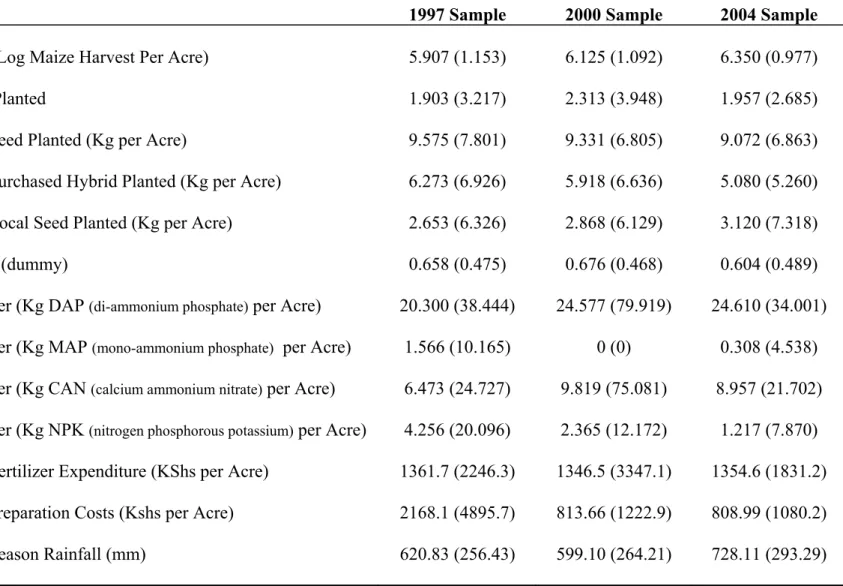
Table 1b shows summary statistics for my sample of households for 1997, 2000 and 2004. There are interesting trends in fertilizer use. There are 26 di¤erent types of fertilizer reported as being used. Table 1b shows only four types (di-ammonium phosphate (DAP), calcium ammo-nium nitrate (CAN), nitrogen phosphorus potassium (NPK) and mono-ammoammo-nium phosphate (MAP)). Table 1c breaks out some of these variables by hybrid/non-hybrid use for the three periods of data. Yields are lower across the board in the non-hybrid sector (the p-values on the t-tests are 0.000 in each period). However, a lot of the other variables look quite similar in means (p-values on the t-tests are often above 5%), except for fertilizer use and main season rainfall.
4
Modeling Adoption Decisions
In this section, I outline a model of adoption decisions that allows for both absolute and com-parative advantage in the selection process determining who uses the hybrid maize technology. Throughout this section, I refer to hybrid maize as the relevant technology, though the empirical model will allow for generalizations to this, mostly with respect to the use of fertilizer.
9
Kenya National Cereals and Produce Board, the marketing board supporting these policies, managed to accrue losses on the order of 5% of the country’s GDP in the 1980’s (Smale and Jayne (2003)).
1 0
There are numerous studies of the impacts of the cereal sector reforms and liberalization, see Jayne et al (2001). Karanja, Jayne and Strasberg (1998) look at the productivity impacts and Jayne, Myers and Nyoro (2005) at the e¤ect on maize prices over 1990-2004. Hassan, Mekuria and Mwangi (2001) show the …ve fold increase in private seed companies between 1992 and 1996, also documented by Kamau (2002) who points out important legislative and regulatory constraints during this time. Finally, Nyoro, Kiiru and Jayne (1999) look at the evolution of di¤erent types of maize traders post-liberalization and Wanzala et al (2001) describe in detail how the private sector has taken over the supply of fertilizer.
1 1
Karanja (1996) states that “newly released varieties in 1989 had smaller yield advantages over their prede-cessors than the previously released ones... research yields were exhibiting a “plateau e¤ect””. Examples he gives are KSII, which was followed by H611 (40% yield advantage), then H622 (16%) and then H611C (12%). H626 which had a 1% yield advantage over H625 was released eight years later.
There are two technology options available to farmers: to plant either a hybrid maize variety or a traditional (non-hybrid) variety12. Say the production functions at any point in time for a farmer are of the Cobb-Douglas form
YitH = e Ht 0 @ k Y j=1 X H j ijt 1 AeuHit (1) YitN = e Nt 0 @ k Y j=1 X N j ijt 1 AeuNit (2)
where the outcome variables, YitH and YitN, are the yields (output per acre) at time t when farmer i uses hybrid or non-hybrid maize respectively13. Throughout, H is used to represent the use of hybrid maize andN the use of non-hybrid. TheXijt’s represent various other inputs (wherej indexes the input), such as fertilizer, labor, rainfall, etc., as well as province dummies. The indexing of Xijt by both i and t is quite general as some of the inputs may only vary by households (such as average long term rainfall). The production functions for hybrid and non-hybrid maize have di¤erent parameters on the inputs, i.e. theXijt’s have di¤erent coe¢ cients in the production functions (indicated by H and N) to allow for complementarity between the maize variety used and the inputs. However, I do assume that the same set of potential inputs are used to grow both hybrid and non-hybrid maize. Finally, theuHit anduNit are sector-speci…c errors that may be the composite of time-invariant household characteristics and time-varying shocks to production. I will consider some speci…c decompositions of theseuH
it and uNit factors below.
Taking logs of equations(1) and (2)above,
yitH = Ht +Xit0 H +uHit (3)
yitN = Nt +Xit0 N +uNit (4)
where yHit and yitH are the logs of yields, the Xit’s have been rede…ned to represent the logs of the inputs. The gain in yields per acre from planting hybrid maize is
Bit=yitH yNit = Ht Nt +X
0
it( H N) +uHit uNit (5)
In this framework, we can start to think about what drives adoption decisions. The simplest 1 2In principle, hybrid use could be a continuous variable as farmers plant quantities of hybrid seed. However, in my sample very few farmers actually plant both hybrid and traditional varieties in a given season. For example, in 1997 only 2% of households planted both hybrid and traditional varieties of maize. Since taking hybrid use to be a binary decision simpli…es the problem dramatically, I use this framework throughout.
1 3The yield equation that I specify is driven mainly by data constraints since the measurement of farm inputs and their prices is di¢ cult. This does not allow direct estimation of a pro…t function. However, maize prices are captured by province and year dummies included in the speci…cation of my yield function. As a result, the log yield regression I estimate captures the bene…ts of hybrid on percentage yields and thus revenues, holding constant my input measures.
decision to adopt would be based on a comparison of the yields under hybrid and non-hybrid maize, such that hit = 1 if yHit > yitN and hit = 0 if yHit yitN, where hit = 1 represents the use of hybrid andhit= 0 the use of non-hybrid. This is the basic implication of the Roy (1951) selection model14 in terms of yields. The Roy model relies on comparisons of wages, or net bene…ts but the conceptual framework it provides can be applied to productivities (as suggested by Mandelbrot (1962)).
The strict Roy model therefore implies that
yitH yN it >1forhit= 1 and y H it yN it 1 forhit= 0 (6)
More generally, for any two individualsiandj using hybrid and non-hybrid maize respectively,
yHit yN it hit=1 > y H jt yN jt ! hjt=0 (7)
Equation (7) implies sorting based on comparative advantage15. The yield maximization rule given by the Roy model in equation(6)therefore imposes comparative advantage.
In the Roy model setup, the adoption decision is based purely on a comparison of yields under hybrid and non-hybrid maize such that
hit(yit) = 1 yitH yitN 0 = 1 h
( Ht Nt ) +Xit0 H N +uHit uNit 0
i
(8)
where1[:]represents an indicator function of whether the expression in brackets holds true. This model of selection can be generalized whereby yield maximization is replaced by income maximization or even a more general selection rule. This is important as it allows for both observed and unobserved costs as well as other factors like tastes/preferences16 to drive the adoption decision. This makes sense in the case of hybrid maize, given its properties. For my scenario, it is important to note two properties of hybrid maize. It increases mean yields as well as reduces the variance in yields, as it can be more pest and drought resistant than traditional varieties.
These two characteristics of hybrid maize are illustrated clearly in Figures 6a, 6b and 6c. The …gures show the conditional distributions of yields across farmers who use hybrid and those who do not for each of the three periods of data I use. It is clear from these …gures that the mean of the hybrid yield distribution lies to the right of that of non-hybrid yields. The hybrid yield distribution also has a lower variance than the non-hybrid yield distribution (the standard
1 4
Also see Heckman and Honore (1990) and Borjas (1987). 1 5
The de…nitions and implications of absolute and comparative advantage as sorting mechanisms have been outlined by various labor economists (see Willis (1986), Green (1991), Sattinger (1993) and Carneiro and Lee (2004)).
1 6One hypothesis for the lack of adoption and the persistence of non-hybrid maize is di¤ering tastes of hybrid and non-hybrid maize, as in Latin America. This is unlikely in Kenya where the di¤erent maize varieties have a uniform price and no distinction in the market.
deviations of the two distributions are signi…cantly di¤erent with p-values on the null of equal standard deviations of 0.000 in each period). These …gures highlight an important property of hybrid maize: it eliminates the lower tail of the distribution of outcomes under non-hybrid maize. This is the main motivation for my model of heterogeneous returns. It is clear that the farmers who would bene…t the most in terms of yields would be those at the lowest end of the non-hybrid distribution of yields - the bad outcomes would be muted under hybrid.
The generalized Roy model allows for maximization of an underlying bene…t function that is far more general than that in equation(8) so that hit = 1iffH(yitH; ZitH)> fN(yitN; ZitN) where
Zitj represents sectorj(j2H; N)costs and factors that a¤ect adoption, including the covariates in theXit’s. The simplest version of this bene…t function would be a pro…t maximization rule. When output prices are the same for hybrid and non-hybrid maize, yields and pro…ts di¤er only by (real) input costs. Throughout the empirical work, I will estimate yield functions, usually controlling for complete input use. My data on inputs is not always at the crop level, but at the …eld level so that calculating maize pro…ts directly is not as straight forward. The speci…cation I use that estimates yield functions controlling for input use is close to estimating pro…t functions. The more general version of a hybrid bene…t function for risk-neutral farmers allows for unobserved costs and factors that are not in the yield equation to a¤ect the adoption decision. These are the components of the Zit’s over and above the Xit’s that are in the yield equation. Examples of variables that may be in this set ofZit’s that are not in the yield equation and are not tastes include the distance from a household to the seed/fertilizer distributor and measures of the availability of seed for a household in any period. Such measures of seed/input availability clearly a¤ect the costs of planting hybrid maize (over and above the observed costs, which are in the Xit’s) and can therefore a¤ect the adoption decision from period to period. In the case of this generalized Roy model, any pattern of sorting is possible and the joint distribution
f(yH; yN) is required to understand the patterns of sorting and comparative advantage (the standard program evaluation problem)17.
In particular, I can write the selection rule for a generalized Roy model for yields in terms of a binary choice based on the latent variable,hi, as
hit(yit) = 1 [hit 0] = 1 h
Zit0 +usit 0i (9)
wherehit is the binary adoption decision with respect to hybrid maize andhit is the latent net bene…ts of planting hybrid maize. us
it is the selection error (the unobservable heterogeneity in the adoption selection equation) and theZit include not just theXit’s from the yield equations, but also the costs and other covariates that may a¤ect the adoption decision. The higher usit
in equation (9), the more likely the farmer is to plant hybrid maize. Comparing this to the strict Roy model (without costs) where the adoption decision was driven purely by di¤erences in yields,hit would just beyitH yitN and usit would beuHit uNit.
1 7
The generalized Roy model still imposes the restriction that the selection rule can be expressed as a single index function. I consider the appropriateness of this restriction when I discuss my results.
Using a generalized yield function of the form
yit=hityHit + (1 hit)yitN (10)
I can substitute in equations(3)and (4) to get
yit= Nt + ( Ht Nt )hit+X
0
it N +X
0
it( H N)hit+uNit + (uHit uNit)hit (11)
Equation (11) illustrates the standard selection problem. If farmers know all or some part of the errorsuHit anduNit and act on what they know, then the decision to adopt hybrid,hit, will generally be correlated with these errors (and hence with the composite erroruNit+ (uHit uNit)hit in equation(11)). The OLS estimate of Ht Nt (and of the average treatment e¤ect) is therefore biased, with the bias composed of both a selection bias and a sorting bias (see Heckman and Li (2003)). For example, it may be the case that the farmers who plant hybrid may just have higher soil quality land and/or better farm management (all of which are unobservable). Heterogeneity of this …xed unobservables form has been emphasized in the literature, in particular with respect to farm management (see Mundlak (1961)), productivity of farmers, and soil quality (see Conley and Udry (2003) and Tittonell (2003)). In addition, there may even be heterogeneity in returns to hybrid maize such that the farmers with the high returns to hybrid maize are the ones who plant it. The average returns to hybrid maize computed by comparing farmers who plant hybrid to those who do not are therefore overstated. My aim is to present a model that can account for both these ideas.
In equation (11), the correlation of hit with (uHit uNit) is an issue. I will start with a general decomposition of the uHit and uNit errors to allow for the possibility that the expected gain to hybrid varies across farmers. The thought experiment is to consider a farmer i who experiences low yields (say in the bottom quartile) when he plants non-hybrid maize. This can be either permanent or transitory low yields - I will be more speci…c later. For this farmer i,
yNit < ct wherect is the percentile cut-o¤ to be in the bottom quartile of non-hybrid yields. His percentage gain in yields is given by (assuming noXit’s for simplicity)E yitH yNit jyitN < ct =
H
t Nt +E uHit uNit jyitN < ct . Similarly, for a farmer who experiences high yields under non-hybrid maize (in the upper quartile, say) so that yNit > kt, his expected gains will be
E yitH yitN jyitN > kt = Ht Nt +E uHit uNit jyitN > kt . I want a structure on the errors,
uHit anduNit, that allows these two expected gains to bedi¤ erent given the return to hybrid looks higher for the farmers in the lowest quartile of the non-hybrid yield distribution.
I therefore consider the following factor structure on the errors18:
uHit = Hi + Hit (12)
uNit = Ni + Nit (13)
1 8
This assumption is similar to the factor assumptions made in Carneiro, Hansen and Heckman (2003), except that I exploit the panel nature of the problem and assume the correlated factors are time-invariant.
The Hit and Nit are assumed to be uncorrelated with each other, as well as with the Xit’s and
Zit’s, unlike the Hi and Ni . This assumption amounts to the transitory errors Hit and Nit not being allowed to a¤ect the farmer’s decision to use hybrid, though the Hi and Ni will. The timing of the production of maize and the fact that it is all rain fed is important here. Farmers are assumed to know their Hi and Ni , but not the Hit and Nit. The seed type (hybrid or non-hybrid) is usually …xed before the it shock is realized. Most farmers plant right before the onset of rains or at the onset of rains (though this is late), but the extent of the rains is unknown. Inputs such as labor and fertilizer may be correlated with the shock, for example rainfall, but the key is that I observe rainfall. So, conditional on the covariates a¤ecting yields I have in my data (most importantly, seasonal rainfall), the assumptions underlying the Hit and Nit are more defendable.
The above structure on the errors allows for maize variety speci…c unobservables, Hi and N
i , to a¤ect yields under hybrid and non-hybrid maize respectively. However, it is only possible to identify a relative relationship between the Hi and Ni unobservables. It is this relative relationship that leads to the idea of comparative advantage in technology adoption and what role this comparative advantage plays, if any, in returns to hybrid technologies.
Substituting the factor structure on the errors into the yield equations in (3)and (4), I get
yHit = Ht + iH +Xit H + Hit (14)
yNit = Nt + iN +Xit N + Nit (15)
Following Heckman and Honore (1991), Lemieux (1998) and others, I use the linear projections of the Hi and the Ni on ( Hi Ni )as follows
H
i = bH( Hi Ni ) + i (16)
N
i = bN( Hi Ni ) + i (17)
where, by construction, the projection coe¢ cients are bH = ( 2H HN)=( 2H + 2N 2 HN),
bN = ( HN 2N)=( 2H + 2N 2 HN) and HN cov( Hi ; Ni ), H2 V ar( Hi ), and 2N
V ar( Ni )19. I de…ne the i to be the absolute advantage as its e¤ect on yields does not vary by the choice of hybrid/non-hybrid. I de…ne Hi Ni to be the comparative advantage gain from growing hybrid, which is orthogonal to the absolute advantage by construction. I can then re-de…ne this comparative advantage gain to be i as follows:
i bN( Hi Ni ) (18)
This is just a rede…nition of the sector speci…c unobservables Hi and Ni . The i serves as a 1 9
The i’s in equations(16)and(17)are the same. Subtracting equation(17)from equation(16)implies that H
i Ni = (bH bN)( Hi iN). For the i’s to be equal across sectors,bH bN must be equal to1, which is
easily shown: bH bN =
2
H HN HN+ 2N
2
measure of comparative advantage in my model. Recall that it is possible to identify only the relative e¤ect of i in the hybrid sector, see Carneiro, Hansen and Heckman (2003). Allowing
bH=bN;equations (16)and (17)become
H
i = i+ i (19)
N
i = i+ i (20)
Substituting these back into equations(14) and(15),
yHit = Ht + i+ i+Xit H + Hit (21)
yNit = Nt + i+ i+Xit N + Nit (22)
The expected gain for a farmer from using hybrid is now a function of both observed and unobserved household characteristics:
Bit=yHit yitH = ( Ht tN) + ( 1) i+Xit0 ( H N) (23)
These descriptions of the logarithmic production functions for the case of heterogeneous returns map back into a generalized version of the Cobb-Douglas production functions I started
with so thatYitH =e ie ie H t k Q j=1 X H j ijt !
e Hit and similarly forYN
i except without thee i term. The motivation for this structure of production functions comes from the fact that hybrid maize increases mean yields and reduces the variance in yields. We would expect individuals who are in the lower tail of the non-hybrid distribution (who have bad outcomes) to bene…t the most from the use of hybrid maize. The production functions illustrate these properties directly: when < 1, farmers with i <0 will have high rewards from hybrid maize (and low rewards if > 1), while farmers with i >0 will have lower rewards from hybrid maize (vice versa if
>1).
I can substitute equations(19)through(22)into the generalized yield equation(10)to derive
yit= Nt + i+ ( tH Nt )hit+Xit0 N + ihit+Xit0 ( H N)hit+"it (24)
where ( 1)is the coe¢ cient on the household speci…c comparative advantage component i and i i+ i. "it is assumed to be the unanticipated component of yields where "it = N
it + ( Hit Nit)hit. The coe¢ cient on hit, i, depends on the unobserved household-speci…c e¤ect i, implying a random coe¢ cient model.
The coe¢ cient on hit, i, is correlated with decisions to adopt (i.e. hit itself). Thinking in terms of the generalized Roy model framework, the household-speci…c expected gain Bit is allowed to enter the latent index determining sector choice, hit. Hence, the coe¢ cient i is generally correlated with the dummy variablehitif agents use their expected gains from growing hybrid in deciding whether or not to plant hybrid. This framework implies a correlated random
coe¢ cient (CRC) model, which I show in the empirical work is a generalization of Chamberlain’s (1984) correlated random e¤ects (CRE) model where household-speci…c intercepts are allowed to be correlated withhit. The CRC model allows both the household-speci…c intercepts as well as household-speci…c slopes/returns to be correlated with hit. As I discuss in detail, this model can be estimated via methods similar to those introduced by Chamberlain (1984).
i and i are uncorrelated by construction, and since the household-speci…c slope is i, the covariance between individual speci…c slopes and intercepts in the yield function is:
cov( i; i) = 2 (25)
The structural coe¢ cient therefore determines whether high intercept households also have the higher returns to hybrid maize. If > 0, then > 1, and the use of hybrid in‡ates the role of comparative advantage in the hybrid sector. In the long run, this would lead to greater inequality in yields in the overall economy.
Equation (24)is a generalization of the household …xed e¤ects model. To illustrate this, let
= 1so that there is now the same …xed unobservable heterogeneity (for example, due to farm management, farmer productivity or soil quality) that a¤ects yields irrespective of the type of maize seed planted. This imposes very speci…c assumptions on the error structure, in particular thatuHit = i+ Hit anduNit = i+ Nit and that the di¤erence ( Hit Nit) must be independent of the selection rule. This implies that the timing of the decision to use hybrid maize at any point in time is independent of the yield di¤erence facing a farmer at that time.
The yield function corresponding to this error structure is the …xed e¤ects version of equation
(24):
yit= Nt + i+ ( Ht Nt )hit+Xit0 N +Xit0 ( H N)hit+"it (26)
where"it= Nit + ( Hit Nit)hit. The expected gain to growing hybrid is therefore:
Bit = ( Ht Nt ) +Xit0( H N) (27)
In this …xed e¤ects model, the expected gain from hybrid in equation (27) can vary across households as long as it is a function of the observableXit’s. But, the unobservable heterogeneity or …xed e¤ect i is restricted to a¤ect yields identically whether or not a farmer uses hybrid. The …xed e¤ect therefore does not appear in equation (27). The …xed e¤ects yield function can be estimated from two periods of panel data on the same farmers under the assumption that, conditional on the i, the error in the yield function is uncorrelated with the decision to adopt hybrid maize. This requires that the source of heterogeneity driving the endogeneity must manifest itself in an i that is …xed across households and that does not vary by the hybrid/non-hybrid choice.
The main contribution of this paper is to relax the assumption that the return to hybrid maize varies by only observable dimensions across households. I draw on recent empirical studies in labor economics that allow for generalizations to the …xed e¤ects model, and use the framework
described above that allows for comparative advantage in the adoption decision. Advances in techniques have been made in the context of experimental data (for example, Heckman, Smith and Clements (1997)) and in cross sectional data where the covariate of interest is a stock variable like schooling. I use the panel nature of my data and build upon the approaches of Lemieux (1993, 1998) and Card (1996)20. To estimate the model in equation (24), I generalize
the multivariate regression/minimum distance approach of Chamberlain (1984) to allow for heterogeneous coe¢ cients.
5
Baseline Results
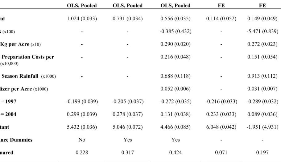
I begin the empirical work by looking at the OLS and household …xed e¤ects speci…cations as a baseline to the heterogeneous returns model. Table 3 shows these OLS and household …xed e¤ects results for speci…cations with and without covariates. The OLS and household …xed e¤ects results reported here are for a simpli…ed version of equation (26):
yit= + hit+Xit0 + i+uit (28)
Comparing this to equation (26), allowing Ht Nt t, I have assumed that t = 8t. In addition, I have assumed that H = N = . I will relax the latter of these assumptions in later results. The former can be relaxed but relaxing it is empirically unimportant - the results from the more complicated model that allows for time-varying ’s are similar so I report results for the simpler model throughout.
The OLS estimates in the …rst column of Table 3 are extremely large and positive: households that plant hybrid maize tend to have much higher maize yields, on the order of 100% higher. Also note the strong time trends in yields for my sample of households over this period. Adding province dummies in the second column of Table 3 decreases the coe¢ cient on hybrid, as there are strong di¤erences across provinces in both yields and hybrid use. In the third column, I add covariates to the speci…cation. The purpose of these covariates is to control for other household variables that could a¤ect yields, and that may be correlated with the use of hybrid maize, mostly inputs. They include land acreage, fertilizer (results are robust to whether quantities or total expenditure are used), land preparation costs, seed quantity, variables that measure labor inputs (both hired and family labor where possible), long term mean seasonal rainfall, current seasonal rainfall, year dummies and province dummies. Adding these covariates decreases the OLS coe¢ cient further, though it is still quite large at56%. The fourth and …fth columns of Table 3 report the household …xed e¤ects results. The coe¢ cient on hybrid decreases dramatically, though with covariates the di¤erence between the OLS and …xed e¤ects is less substantial. There is still a substantial return to hybrid maize even within households, controlling for …xed unobservable heterogeneity and a wide set of covariates, on the order of15%.
2 0
Some of these issues have been debated in the literature on the return to unionization, see Vella and Verbeek (1998), Green (1991) and Robinson (1989) for examples.
This household …xed e¤ects framework is restrictive in the assumptions it imposes on the adoption process and the comparison of the adopters and non-adopters. A consequence of the restrictions it imposes is that there is assumed to be no di¤erence between farmers who switch into the use of hybrid and those that switch out of the use of hybrid. The i allows some farmers to be more productive overall (higher i), but the di¤erence across the hybrid and non-hybrid sectors is the same for all farmers, irrespective of their transition histories. Apart from the permanent component in the outcome equation, i, the adoption decision cannot depend on observed outcomes except under restrictive assumptions on the transitory component (see Ashenfelter and Card (1985)). Such assumptions can be motivated by myopia or ignorance of the potential gains from planting hybrid, but they are unrealistic here21. In addition, as emphasized by Card (1998), the …xed e¤ects model requires that the selection bias for a given characteristic, such as farmer experience or soil quality, must be of the same sign for all individuals. It does not allow, for example, selection into hybrid to be positive for people with low education, say, but negative for those with high education.
For various agronomic and economic factors, such as the slow spread of information and the credit constraints that are alluded to in the literature, it is reasonable to allow for a distribution of returns to the technology that relies on both observed and unobserved factors. The household …xed e¤ects model may therefore not be appropriate for the question at hand. The rest of this section describes tests of the household …xed e¤ects model, and some intuitive evidence for selection and heterogeneity in returns.
5.1 Two Period CRE Model
The household …xed e¤ects estimates are consistent only under the assumption of strict exo-geneity of the errors. Chamberlain’s CRE approach provides a basis for testing this assumption (see Chamberlain (1984) and Jakubson (1991)). I illustrate the simple two period, no covariates CRE model, for which the data generating process is given by
yit = + hit+ i+uit (29)
The assumption of strict exogeneity of the errors is:
E(uitjhi1; :::; hiT; i) = 0 (30)
CRE illustrates how the …xed e¤ects model is overidenti…ed. Replace the …xed e¤ect, i, by its linear predictor based on the history of the covariates:
i= 0+ 1hi1+ 2hi2+vi (31) 2 1
Hybrid maize was introduced in the 1960’s, with widespread use of extension services to promote the tech-nology. See Evenson and Mwabu (1998).
where the projection error vi is uncorrelated withhi1 and hi2 by construction, and the ’s are the projection coe¢ cients. Substituting this linear projection into the yield equation,
yit= + hit+ 0+ 1hi1+ 2hi2+vi+uit (32)
Let it=vi+uit whereE[ ithi1] =E[ ithi2] = 0. For each time period, therefore:
yi1 = ( + 0) + ( + 1)hi1+ 2hi2+ i1 (33)
yi2 = ( + 0) + 1hi1+ ( + 2)hi2+ i2 (34)
These are the structural yield equations for each period. I estimate reduced form yield functions for each period of the form
yi1= 1+ 1hi1+ 2hi2+ i1 (35)
yi2= 2+ 3hi1+ 4hi2+ i2 (36)
Equations (33) through (36) show how the …xed e¤ects model is overidenti…ed. From the four reduced form coe¢ cients, 1; 2; 3 and 4, I can estimate the three structural parameters, 1; 2 and using minimum distance. It is important to note that estimating the CRE model does not require a speci…cation of the conditional expectation of the i. Neither does it require knowledge of the true conditional expectation of the i.
The intuition behind the identi…cation of the CRE model comes from the underlying as-sumption of the strict exogeneity of the errors. If the …xed e¤ects model is valid, then the only way the history ofhit (both past and future) a¤ects the current outcome is through the house-hold level unobservable, i. The identi…cation of comes from those individuals who switch hybrid status hit during the course of the panel. Conditional on i and the included regressors, the switching behavior is taken to be exogenous and driven by transitory factors uncorrelated with the rest of the model. This is testable with panel data as described above. The structural estimates are overidenti…ed even in the two period case. The minimum distance estimator of the structural parameters is also the minimum 2 estimator if the weight matrix used is the inverse of the variance covariance matrix of the reduced form coe¢ cients. This is called the optimal minimum distance (OMD) estimator. If the identity matrix is used as the weight matrix in-stead, the estimates are referred to as equally weighted minimum distance (EWMD) estimates. The OMD estimates are e¢ cient, but they can be biased in small samples and can therefore be out-performed by EWMD (see Altonji and Segal (1996)). Throughout, I report both sets of estimates, as well as the 2 statistics on the OMD problem, which are just the value of the minimand in the OMD problem.
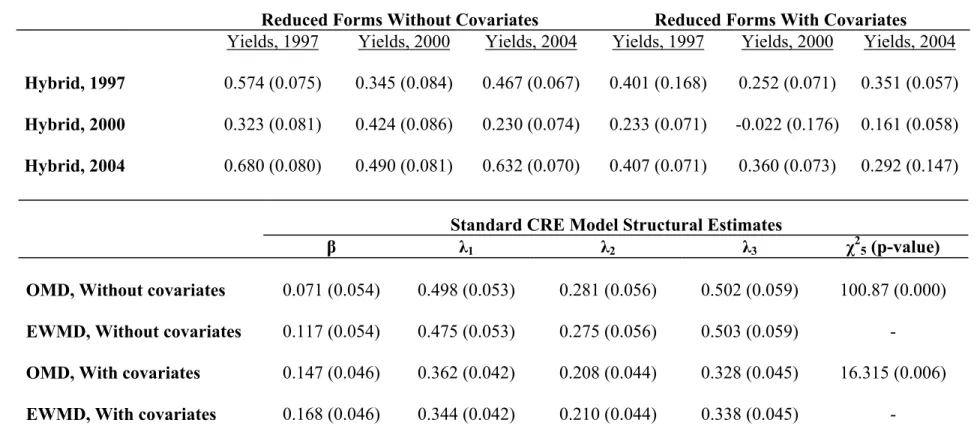
Estimates of the CRE model for three periods, both with and without covariates are shown in Table 4. In the CRE model, covariates can be treated as either exogenous or endogenous. Exogenous covariates enter the model in equation (29), but are assumed to be uncorrelated with the …xed e¤ect so that they do not enter the projection in equation (39). Endogenous
covariates, on the other hand, are correlated with the …xed e¤ect and enter the projection. The CRE model therefore allows tests of whether covariates are endogenous. I report estimates where all covariates (other than the choice to plant hybrid) are assumed to be exogenous, though allowing for endogenous covariates does not change the results.
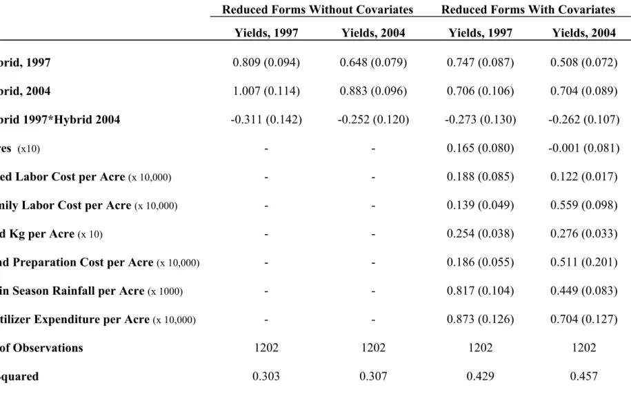
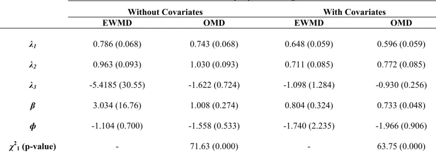
Table 4 shows both the reduced form and structural estimates for various speci…cations. The reduced forms in the upper panel of Table 4 give nine reduced form parameters (not including the constants or covariates), from which I use minimum distance to estimate the four structural estimates, shown in the lower panel of the table. Three of these structural estimates are the ’s from the linear projection of the …xed e¤ects and the fourth is the estimate of the return to hybrid, . The CRE estimates of in all cases are very close to the household …xed e¤ects estimates in Table 3, as expected. The OMD and EWMD estimates of are quite similar, all within sampling error of each other. The last column in the lower panel of Table 4 shows the 2 values on the overidenti…cation test. In all cases, I can reject the null that the minimum distance restrictions hold. This overidenti…cation test is an omnibus test. It has low power against any speci…c alternative, but it does have power against many alternatives. It is therefore not surprising that I am able to reject the overidentifying restrictions.
5.2 Preliminary Evidence of Heterogeneity
To motivate my framework of heterogeneous returns, I report some tests for heterogeneity (see Heckman, Smith and Clements (1997)). These arepurelyfor illustrative purposes, as they ignore the role of selection and assume that the data is experimental, i.e. that farmers using hybrid and non-hybrid maize are the same on average. This is an extremely strong assumption. Let the conditional yield distributions for the adopters and non-adopters of hybrid be FH(yHjh = 1)
andFN(yNjh= 0)respectively (shown in Figures 6a, 6b and 6c). The conditional distributions allow us to bound the unknown joint distribution of interest,F(yH; yNjh= 1), via the Frechet-Hoe¤ding bounds22 which also bound the variance,V ar(yH yN). A test of whether the lower bound of V ar( y) is signi…cantly di¤erent from zero is a test for heterogeneity in returns. I can look at whether each percentile of the hybrid and non-hybrid yield distributions di¤ers by a common constant with the null hypothesis H0 : q(yH) q(yN) = k for all q such that 0
q 10023. Figures 7a, 7b and 7c show the di¤erences in percentiles of the returns distributions,
assuming perfect positive dependence, and Figures 8a and 8b show similar plots for my samples of joiners (farmers who do not use hybrid one period but do the next) and leavers (vice-versa). Appendix Table A2 shows the full set of results where I can reject the null hypothesis above.
2 2
The Frechet-Hoe¤ding bounds are given by: max FH(yH jh= 1) +FN(yN jh= 1) 1;0 F(yH; yN jh= 1) min[FH(yH jh= 1); FN(yN jh= 1)] 2 3
I need to make assumptions about the dependence in the hybrid and non-hybrid conditional yield distrib-utions. The two extreme dependence assumptions are perfect positive dependence (the individual at the 99th percentile in the hybrid distribution would be at the 99th percentile of the non-hybrid distribution had he not planted hybrid) and perfect negative dependence, where the percentile rankings are assumed to be reversed.
5.3 Evidence of Selection
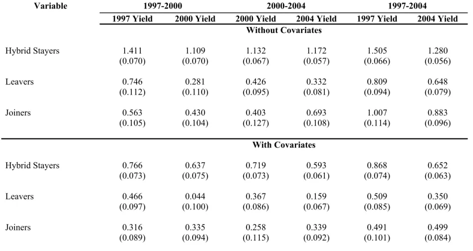
Assuming away selection is hardly tenable; in Table 5, I look for evidence of selection. I split the adoption history into dummies describing the transitions of households across technologies over the three periods. The idea is to look at whether households with di¤erent transition histories have di¤erent returns in terms of yields to planting hybrid (see Card and Sullivan (1988)). To understand transition histories, I de…ne a “joiner” to be a farmer who does not plant hybrid the …rst period, but does the next, and a “leaver”to be a farmer who plants hybrid one period, but not the next. Similarly, I de…ne a “hybrid stayer”to be a farmer who plants hybrid in both periods and a “non-hybrid stayer” to be one who plants traditional varieties in both periods. Under a household …xed e¤ects model, the selection is re‡ected by the coe¢ cients on the stayers and leavers in the periods in which they are not growing hybrid.
I look at each pair of periods in my data and compare yields for the hybrid and non-hybrid stayers, the joiners, and the leavers in each of the two periods separately to learn about the extent of selection. For example, the …rst two columns in Table 5 look at the transitions of households over 1997-2000, with the omitted group being the non-hybrid stayers. The …rst and second columns of this table compare the yields in 1997 and 2000 for hybrid stayers, joiners and leavers in 1997 and 2000 separately. If there was no selection at all (not even via a household …xed e¤ect), we would expect the coe¢ cient on the leavers in the yield equation for 1997 to be no di¤erent from the coe¢ cient on the stayers, and also no di¤erent from the coe¢ cient on the joiners in the yield equation for 2000. Similarly, the coe¢ cient on joiners in the yield equation for 1997 would be no di¤erent from zero, as should the coe¢ cient on the leavers in the yield equation for 2000. Hence, the coe¢ cient on the leavers and joiners across the two yield equations illustrates the extent of selection. Table 5 reports similar estimates for 2000-2004 and 1997-2004. The hybrid stayers uniformly get the largest yields and the leavers and joiners get very di¤erent changes in yields when they switch their adoption status.
In Table 6, I look for heterogeneity in returns to hybrid seed along observable dimensions. This relaxes the assumption that H = N = in the OLS and FE estimations reported above. Table 6 reports results for yield functions estimated separately for hybrid and non-hybrid households. I report both the OLS as well as household …xed e¤ects speci…cations. The returns to observables di¤er by the use of hybrid, especially in the cases of fertilizer and rainfall. This holds for both the OLS as well as the household …xed e¤ects speci…cations. The last row of Table 6 reports estimates of the return to hybrid (evaluated at the mean Xit’s) for the case where the returns to observables are allowed to vary across hybrid and non-hybrid use. There is a signi…cant return to hybrid for both the OLS and …xed e¤ects speci…cations, even after allowing for returns to vary by the observables.
6
Estimating a Model with Heterogeneous Returns
The model of heterogeneous returns outlined earlier implies the following econometric model in maize yields for the simple two period, no covariates case:
yit= + hit+ i+ ihit+ it (37)
For simplicity, I focus only on hybrid maize and leave out other inputs to explain the empir-ical strategy and then discuss extensions. The model above24 can be estimated as per Lemieux (1998), using non-linear 2SLS. Instead, I extend the basic Chamberlain CRE approach to a scenario of correlated random coe¢ cients. This may be somewhat easier and allows a 2 overi-denti…cation test, similar to that described above. The next sections are devoted to describing my estimation and identi…cation strategy, keeping in mind the intuition of the CRE approach. I then describe extensions to this basic model and the estimation results.
6.1 Two Period CRC Model
For the simple two period, no covariates case, the yield function is given by equation (37)
above. The key identifying assumption here is that, conditional on the comparative advantage component ihit (and the covariates in the more general speci…cations), the unanticipated component of yields, "it, is not correlated with the decision to adopt. Remembering that i
i+ i, where i and i are orthogonal, I re-write equation (37) as
yit = + i+ hit+ ihit+ i+"it (38)
Using the same idea as CRE, I linearly project the i’s onto the history of the hybrid decisions, as well as their interactions so that the projection error is orthogonal tohi1 andhi2 individually as well as to their product,hi1hi2 by construction25. The projection is given by
i = 0+ 1hi1+ 2hi2+ 3hi1hi2+vi (39) 2 4This empirical model is similar to models of individual speci…c heterogeneity in Heckman and Vytlacil (1997), Card (2000, 1998), Deschênes (2001), Carneiro, Hansen and Heckman (2001), Carneiro and Heckman (2002), and Wooldridge (1997). Lemieux (1998) has a very similar model to look at whether the return (in terms of wages) to both observables and unobservables varies by union sector membership.
2 5
The projection I use here is di¤erent from what CRE uses. If I use the simple CRE projection, i =
1hi1+ 2hi2+vi, and substitute this into the yield function,
yit= 0+ 1hi1+ 2hi2+ hit+ 0+ 1hi1hit+ 2hi2hit+vi+ vihit+uit
Even thoughvi, the projection error, is linearly uncorrelated withhi1andhi2individually, it is generally correlated
with their product,hi1hi2, so thatE[vihi1hi2]6= 0. The projection I use must therefore include the interactions
In addition, I normalize the i’s so that P i = 0. Since hit is a dummy variable, substituting the above projection into the yield equations gives:
yit= + 0+ 1hi1+ 2hi2+ 3hi1hi2+ hit+ 0hit+ 1hi1hit+ 2hi2hit+ 3hi1hi2hit+vi+ vihit+uit (40) For each of the two time periods, the yield functions are:
yi1 = ( + 0) + [ 1(1 + ) + + 0]hi1+ 2hi2+ [ 3(1 + ) + 2]hi1hi2+ (vi+ vihi1+ui1) (41)
yi2 = ( + 0) + 1hi1+ [ 2(1 + ) + + 0]hi2+ [ 3(1 + ) + 1]hi1hi2+ (vi+ vihi2+ui2) (42)
The corresponding reduced forms are:
yi1 = 1+ 1hi1+ 2hi2+ 3hi1hi2+ i1 (43)
yi2 = 2+ 4hi1+ 5hi2+ 6hi1hi2+ i2 (44)
Equations (43) and (44) give six reduced forms coe¢ cients ( 1; 2; 3; 4; 5 and 6), from which I can estimate the …ve structural parameters ( 1; 2; 3; and ) using minimum dis-tance26. The structural parameters are clearly overidenti…ed and the restrictions for the mini-mum distance problem are:
1 = (1 + ) 1+ + 0 2 = 2 3 = (1 + ) 3+ 2 4 = 1 5 = (1 + ) 2+ + 0 6 = (1 + ) 3+ 1 (45)
I now discuss extensions to this basic model and whether the i’s themselves can be recovered from this estimation.
6.2 Extensions
I consider the following extensions:
1. Covariates: all the identi…cation arguments presented above generalize when the model includes covariates. Covariates in the CRE model can be thought of as either exogenous or endogenous, the latter implying that they are correlated with the …xed e¤ects. Allowing for 2 6There may seem to be six structural parameters, given the presence of
0in equations(39)and(45). However,
given the normalization thatP i = 0, then 0 is just a function of the hybrid histories, their interactions and
the other 0s. In particular,
0 = 1hi1 2hi2 3hi1hi2 wherehi1 andhi2 are the averages of the adoption
endogenous covariates in CRE is straight forward: all the leads and lags of the endogenous covariates are included in the projection. The CRC model is slightly more complicated and can become cumbersome. Endogenous covariates are de…ned similarly - they are correlated with the i’s. I allow for fertilizer to be an additional endogenous covariate so that the CRC projection generalizes to
i = 0+ 1hi1+ 2hi2+ 3hi1hi2+ 4hi1fi1+ 5hi2fi1+ 6hi1hi2fi1
+ 7hi1fi2+ 8hi2fi2+ 9hi1hi2fi2+ 10fi1+ 11fi2+vi (46)
where fit for t= 1;2 represents the use of fertilizer in each period. The other covariates enter the problem in such a way that they are exogenous (uncorrelated with the i’s)27.
2. Three periods: this is a simple extension. For space considerations, I do not show the restrictions for the three period model. The problem becomes heavily overidenti…ed with only 9 structural parameters to estimate from the 21 reduced form coe¢ cients for the base case with no other endogenous covariates. However, as covariates are allowed to be endogenous, the model becomes cumbersome.
3. Joint choice variables: the two-sector model presented above (hybrid/non-hybrid) can be extended to multiple sectors. An additional technology use sector, like fertilizer, can be incorporated by thinking of a four sector model (farmers use either both hybrid and fertilizer, neither, one or the other). I simplify it further. In 1997, for example, 76% of households …t into one of two of the possible four sectors, namely using both hybrid maize and fertilizer or neither. So, I estimate an easier model that rede…nes sectors to this joint decision (using both hybrid and fertilizer or not) and looks at the heterogeneity in returns across these two sectors.
6.3 CRC Estimates
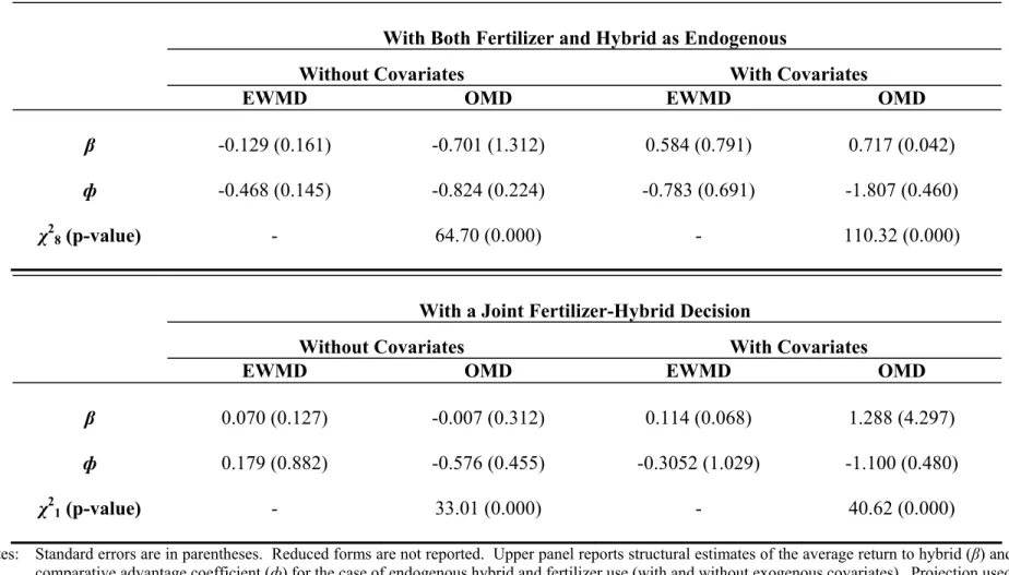
This section describes various estimates of the CRC model. I report estimates for the pure hybrid model described in detail above (with and without covariates) for both the two and three period cases. In addition, I report results for the endogenous covariate and joint hybrid-fertilizer extensions to the basic model that I described in the previous section. Recall that a covariate is described as endogenous if it is assumed to be correlated with the i’s and therefore enters the projection in equations (39) or (46) (similarly, a covariate is exogenous if it is assumed to be uncorrelated with the i’s).
Tables 7, 8a, 8b and 9 present the CRC model reduced form and structural estimates. These tables report both the EWMD and OMD estimates for cases with and without covariates, as
2 7
There is some justi…cation for this. Using the estimates from the pure hybrid problem in Tables 7 and 8, I am able to look at the distribution of predicted i’s and correlate this with the covariates. Of all the covariates,