Topology-aware GPU scheduling for learning workloads in cloud environments

in Cloud Environments

Marcelo Amaral

[email protected]

Jordà Polo

Barcelona Supercomputing Center [email protected]

David Carrera

Barcelona Supercomputing Center Universitat Politècnica de Catalunya

[email protected]

Seetharami Seelam

IBM Watson Research Center [email protected]

Malgorzata Steinder

[email protected]

ABSTRACT

Recent advances in hardware, such as systems with multiple GPUs and their availability in the cloud, are enabling deep learning in various domains including health care, autonomous vehicles, and In-ternet of Things. Multi-GPU systems exhibit complex connectivity among GPUs and between GPUs and CPUs. Workload schedulers must consider hardware topology and workload communication re-quirements in order to allocate CPU and GPU resources for optimal execution time and improved utilization in shared cloud environ-ments.

This paper presents a new topology-aware workload placement strategy to schedule deep learning jobs on multi-GPU systems. The placement strategy is evaluated with a prototype on a Power8 ma-chine with Tesla P100 cards, showing speedups of up to≈1.30x compared to state-of-the-art strategies; the proposed algorithm achieves this result by allocating GPUs that satisfy workload re-quirements while preventing interference. Additionally, a large-scale simulation shows that the proposed strategy provides higher resource utilization and performance in cloud systems.

CCS CONCEPTS

•Theory of computation→Scheduling algorithms;Graph algorithms analysis;Machine learning theory; •Computer systems organization→Cloud computing;

KEYWORDS

Scheduling, Placement, GPU, Multi-GPU, Performance Analysis, Resource Contention, Workload Interference and Deep Learning. ACM Reference format:

Marcelo Amaral, Jordà Polo, David Carrera, Seetharami Seelam, and Malgo-rzata Steinder. 2017. Topology-Aware GPU Scheduling for Learning Work-loads in Cloud Environments. InProceedings of SC17, Denver, CO, USA, November 12–17, 2017,12pages.

DOI: 10.1145/3126908.3126933

Permission to make digital or hard copies of all or part of this work for personal or classroom use is granted without fee provided that copies are not made or distributed for profit or commercial advantage and that copies bear this notice and the full citation on the first page. Copyrights for components of this work owned by others than ACM must be honored. Abstracting with credit is permitted. To copy otherwise, or republish, to post on servers or to redistribute to lists, requires prior specific permission and/or a fee. Request permissions from [email protected].

SC17, Denver, CO, USA

© 2017 ACM. 978-1-4503-5114-0/17/11. . . $15.00 DOI: 10.1145/3126908.3126933

IBM Power8 using NVLink NVIDIA DGX-1 using NVLink

CPU GPU1 GPU2 CPU PCI-e Switch PCI-e Switch GPU1 GPU3 GPU2 GPU4 PCI-e Switch PCI-e Switch GPU5 GPU7 GPU6 GPU8 GPU3 GPU4 NVLink(20GB/s unidirectional) PCI-e v3 x16 (16GB/s unidire.) Inter-socket (e.g., QPI, BW varies)

M E M ME M _{CPU CPU} M E M M E M

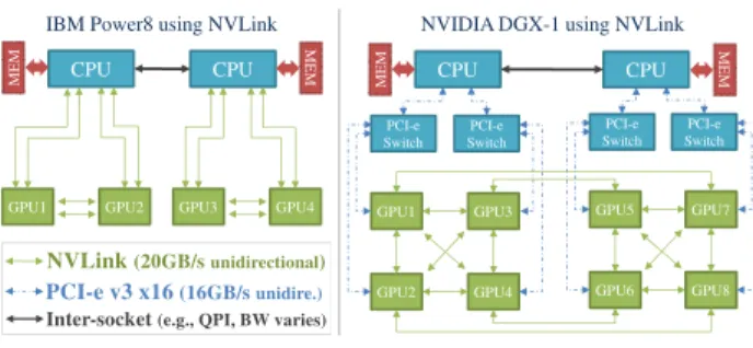
Figure 1: Examples of GPU physical topology.

1

INTRODUCTION

Recent advances in the theory of Neural Networks (NNs), new computer hardware such as Graphic Processing Units (GPUs), avail-ability of training data, and the ease of access through cloud have allowed Deep Learning (DL) to be increasingly adopted as a part of business-critical processes in health care, autonomous vehicles, natural language processing, and Internet of Things. Consequently, many on-line platforms that offer image-processing and speech-recognition systems leveraged by trained DL NNs are emerging to deliver various business critical services, such as IBM Watson [23], Microsoft Project Oxford [31], Amazon Machine Learning [2], and Google Prediction API [16].

Training DL NNs is a computationally intensive process. An image-processing application, for instance, might demand the anal-ysis of millions of pixels in one of many layers of the NN that takes several hours to days of computations [10]. A promising approach to increase the levels of efficiency in processing time and power consumption of the training process is using one or more GPUs. Computing the NNs on multiple GPUs further reduces training times, enables to handle larger amounts of data, and increases the accuracy of the trained models. Hence, multiple GPUs has become a common practice for DL applications [10,18]. Although training on multiple GPUs can deliver many advantages, it presents new challenges in workload management and scheduling for obtaining an optimal performance. The performance depends on both the GPUs and CPUs connectivity on the physical topology, and the application’s tasks communication pattern.

To illustrate this issue, consider Figure1which shows the connec-tivity topology between the GPUs and CPUs for two representatives DL cognitive systems. In these systems, multiple link technologies such as PCI-e and NVLink connect GPUs to each other and GPUs to host CPUs. NVLink offers better bandwidth and lower power

consumption over PCI-e. In the figure, IBM Power8 system consists of four GPUs and two CPUs with two GPUs per CPU socket. The two GPUs on each socket are connected with dual lane NVLink to achieve up to 40GB/s unidirectional bandwidth, and each of the GPUs is also linked to the socket with two lanes of NVLink. The two CPUs are connected via the system bus. NVIDIA DGX-1 has 8 GPUs connected to two CPU sockets. The GPUs are connected over a hybrid cube-mesh topology: the 12 edges of the cube are connected via single lane NVLink, and the diagonals of two of six faces are also connected via NVLink. Each of the GPUs is also con-nected to a PCI-e switch so it can communicate to a GPU that is not connected to it via the NVLink and communicate to the CPU as well.

In these systems, communications can take place directly be-tween devices, in the so-called Peer-to-Peer model (P2P), or it should be routed through the main memory of the processors containing the bus controllers. For example, in the case of DGX-1, the commu-nication between GPU1 and GPU5 will go over the PCI-e switches and the system bus (such as quick path interconnect – QPI). As a result of these complex connectivity topologies between different GPUs, the application performance depends on which GPUs are allocated for computations and how the GPUs are connected to each other (via PCI-e or NVLink).

Additionally, this challenge becomes acute in shared systems, like cloud computing, where multiple applications from different users share the GPUs on the system. At this time, it is uncom-mon to share a single GPU between two applications so sharing here means different applications get different sets of GPUs. Jobs in this environment have varied GPU requirements: some need a single GPU, some need GPUs with NVLink, others need multiple GPUs but communication requirements are minimal, etc. In such environments, cloud scheduler should be able to take the commu-nication requirements of the workloads, consider the topology of the system, consider existing applications and their GPU and link utilization and provision the GPUs for the new workload that meet the workload requirements. This enables users to get access to the resources necessary without worrying about the detailed topology of the underlying hardware. Major cloud providers such as IBM, Amazon, Google, Microsoft, and others provide multi-GPU systems as a service today via virtual machines, and most of them have sys-tems with similar GPU topology described in Figure1; so that job scheduling and resource management becomes critical at the time of running multi-GPU based applications on a shared system. Thus, those systems require the same placement functionality proposed in this work to fully exploit the capabilities of modern cognitive systems. Furthermore, both cloud and HPC systems can benefit from a GPU topology-aware schedule.

In this paper, we present an algorithm with two new scheduling policies for placing GPU workloads in modern multi-GPU systems. The foundation of the algorithm is based on the use of a new graph mapping algorithm that considers the job’s performance objectives and the system topology. Applications can express their perfor-mance objectives as Service Level Objectives (SLOs) that are later translated into abstract Utility Functions. The result of using the proposed algorithm is a minimization of the communication cost,

reduction of system resource contention and an increase in the system utilization.

The major contributions of this paper are:

• Performance characterization of placement strategies and inter-ference from co-scheduled jobs over a modern Power8 system composed of NVLinks. The results show that using pack instead of spread for a job with high GPU communication gives a speedup ≈1.30x. Additionally, the results indicate that co-schedule jobs with high GPU communication instead of running them solo can conduct to a slowdown of≈30% (Section3).

• A topology-aware placement algorithm that places jobs based on its utility with best-effort on preventing SLO violations. Two scheduling policies are defined: TOPO-AWARE-P allowing to postpone the placement of unsatisfied jobs, and TOPO-AWARE that always place jobs when resources are available (Section4). • A prototype evaluation of the proposed algorithm showing the performance improvements that a topology-aware scheduling confers for DL workloads using multiple GPUs. The results show a speedup of up to≈1.30x in the cumulative execution time and no SLO violations compared to greedy approaches (Section5). • A trace-driven simulation to analyze the topology-aware

place-ment algorithm on a large-scale cluster. The results show that the proposed algorithm outperforms the greedy algorithms in the execution time, with no or fewer SLO violations (Section5). Section6discusses the state of the art and related work, and Sec-tion7presents summary, conclusions, and future works.

2

DEEP LEARNING WORKLOADS

This section presents DL frameworks and their characteristics that are relevant for topology-aware scheduling in multi-GPU execu-tions. With the increasing popularity of the DL methods, several deep learning software frameworks have been proposed to enable efficient development and implementation of DL applications. The list of available frameworks includes, but is not limited to, Caffe, Theano, Torch, TensorFlow, DeepLearning4J, deepmat, Eblearn, Neon, PyLearn, among others [3]. While each framework develops different algorithms and tries to optimize various aspects of train-ing, they share similar GPU communication algorithms [42]. This work is focused on one of the most popular frameworks at this time, Caffe, but our results are equally applicable to other frameworks. Various NN models are implemented for Caffe, including AlexNet, CaffeRef (based on AlexNet) and GoogLeNet. We use those mod-els for evaluating the efficacy of the topology-aware scheduling algorithm presented in this paper.

DL frameworks have two main approaches to divide the work-load when using multiple GPUs: data-parallelization and model-parallelization. In data-parallelization, the data is partitioned and spread to different GPUs, and in model-parallelization, the NN model is partitioned, and different GPUs work on different parts of the model, for example, each GPU will have different NN layers of a multi-layer NN. However, while the model-based parallelism is expected to be more communication intensive, it is still uncommon for cloud deployments, and therefore we focused all experiments on data-parallelization. We expect that topology-aware scheduling is even more critical for model-parallelization workloads because of the higher communication requirements.

Additionally, a key parameter that plays a significant role in the communication is thebatch size. It determines how many samples per GPU the NN will analyze in each training step, and directly impacts the amount of communication and computation in each step. The lower the batch size is, the noisier the training signal is going to be; the higher it is, the longer it will take to compute the stochastic gradient descent. Noise is an important component for solving nonlinear problems. Hence, small batches size is a new trend for training DL NNs, which also determines the level of parallelism the NN can reach since the batch size partitions the dataset [6].

The next section presents an evaluation of the impact of different placement strategies on execution time with three different NNs (AlexNet, CaffeRef, and GoogleNet) and each NN with four different batch sizes (tiny, small, medium, big).

3

EVALUATING THE IMPACT OF

PLACEMENT STRATEGIES

In this section, we evaluate two general purpose workload place-ment strategies:packandspread. Later, in Section4, we combine them into the utility function used in our proposed algorithm.

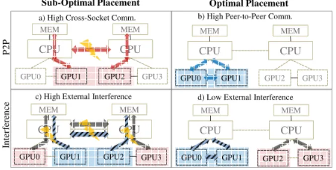
The main sources of performance perturbation on multi-GPU applications are how the allocated GPUs are connected, i.e. the topology, and how much of the shared bus bandwidth other ap-plications are utilizing. To illustrate it, Figure2shows different workload placement strategies that can be defined on top a single machine with hardware topology composed of two sockets and two GPUs per socket (the same topology shown in Figure1for the Power8 system). The GPUs within the same socket are located at a “shorter” distance (from a topology perspective) than the GPUs located across sockets. Besides, GPUs on the same socket can utilize the higher bandwidth and lower latency network (e.g., NVLink) to communicate instead of going over the PCI-e and the QPI links to communicate across CPU sockets.

Sub-Optimal Placement CPU MEM GPU0 GPU1 CPU GPU2 GPU3 Optimal Placement MEM CPU MEM GPU0 GPU1 CPU GPU2 GPU3 MEM a) High Cross-Socket Comm. b) High Peer-to-Peer Comm.

c) High External Interference d) Low External Interference

CPU MEM GPU0 GPU1 CPU MEM GPU2 GPU3 CPU MEM GPU0 GPU1 CPU GPU2 GPU3 MEM P 2 P In te rfe re n ce

Figure 2: Pack vs. Spread, and collocation vs. solo.

Therefore, the first workload placement strategy ispack, which systematically favors minimizing the distance between GPUs, to prioritize the performance of GPU-to-GPU communication. The second workload placement strategy isspread, which attempts to allocate GPUs from different sockets and prioritize the performance of CPU-to-GPU communication. Spread promotes better resource utilization and minimizes fragmentation.

Another factor that impacts the performance of either pack or spread placement schemes is the interference introduced by other applications sharing the system resources. For this reason, the placement algorithms should take not only the static topology of

the system but also the runtime utilization metrics from currently executing applications for scheduling decisions.

Next, we describe the testing platform and evaluate the impact of the placement strategies to allocate GPUs for the DL applications outlined in section2.

3.1

Testing Platform and Configuration

All experiments are conducted on an IBM Power8 System S822LC re-lease, code-named as “Minsky” shown in Figure1. The server has 2 sockets and 8 cores per socket that run at 3.32 GHz and two NVIDIA GPU P100’s per socket. Each GPU has 3584 processor cores at boot clocks from 1328 MHz to 1480 MHz, and 16 GB of memory. Each socket is connected with 256 GB of DRAM. Where the intra-socket CPU-to-GPU and GPU-to-GPU are linked via dual NVLinks that uses NVIDIA’s new High-Speed Signaling interconnects (NVHS). A single link supports up to 20GB/s of unidirectional bandwidth be-tween endpoints. A high-level illustration of the hardware topology is pictured in Figure1and Figure2.

For the software stack, this machine is configured with Red Hat Enterprise Linux Server release 7.3 (Maipo), kernel version 3.10.0-514.el7.ppc64le, Caffe version v0.15.14-nv-ppc compiled with NCCL 1.2.3, CUDA 8.0 and CUDA driver 375.39. All Caffe workloads are configured with a set of images from the dataset used in the 2014 ImageNet Large Scale Visual Recognition Challenge (which is one of the most well-known datasets for image classification and publicly available on the ImageNet competition website).

All experiments were repeated five times. For each experiment, the maximum number of iterations is 4000, except when generating the GPU profile where the iterations are only 40. The iterations are decreased because profiling consumes a lot of memory, and a large profile does not fit in the GPU memory. The tool used to profile the application was the NVIDIAnvprofile. For all workloads, the NN training batch sizes range from 1 up to 128.

3.2

Pack versus Spread

Figure4shows the relative speedup achieved when allocating GPUs within the same socket (pack) or over cross-socket (spread). When the speedup is higher than 1, the application performs better with the pack strategy. The performance depends on both the workload type and the batch size. When AlexNet is configured with batch size 1 or 2, it has a speedup of up to≈1.30x, but for batch sizes larger than 16 both pack or spread have even performance. GoogLeNet has a different behavior than the other NNs with less or no impact, which will be better detailed next.

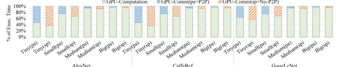
To better explain the cause of the performance delivered by the strategies, the application breakdown is presented in Figure3. The analysis shows the percentage of computation and communication represented in the whole execution time. The results indicate that larger batch sizes significantly increase computation time, while communication time becomes less significant overall.

Taking AlexNet, for instance, when configured with tiny batch sizes, the computation time is≈1s for 40 iterations; with big batch sizes, this time increases to≈66s. The communication time instead remains≈2s for all batch sizes. While NNs with a bigger batch size increases the amount of data exchanged between the GPUs, it starts to spend much longer time performing computation in the GPU

0% 20% 40% 60% 80% 100%

AlexNet CaffeRef GoogLeNet

% o f Ex e c. T ime

GPU-Computation GPU-Comm(pa=P2P) GPU-Comm(sp=No-P2P)

Figure 3: Application breakdown showing the percentage GPU computation and communication in relation to the whole execution time. All workloads have the GPUs allocated using either the pack (pa) or the spread (sp) strategies.

0.9 1.0 1.1 1.2 1.3 1 2 4 8 16 32 64 128 S p ee d u p

Batch Size (per-GPU) AlexNet CaffeRef GoogLeNet

Figure 4: Pack (P2P) vs. Spread (No-P2P). When the speedup is higher than 1, pack is better than spread.

for each batch step. Hence, the communication starts to be less frequent with bigger batch sizes. On the other hand, smaller batch sizes require many more steps to process the whole dataset and then require more frequent communication. This behavior can be verified with the NVLink bandwidth usage in Figure5.

The communication frequency directly impacts the usage of the NVLink bandwidth. The NN configured with a small batch size reaches higher NVLink bandwidth usage≈40GB/s, while the NN with a bigger batch size barely reaches≈6GB/s, as in Figure5(the NVLink bandwidth calculation is described later in Section5.1).

GoogLeNet is the less intuitive case. Since this NN contains sizable neural network layers, and typically the intensity of com-munications depends on the amount of information exchanged between the layer, it is expected that GoogLeNet performs more communication than the other NNs. Nonetheless, GoogLeNet per-forms less communication because of its Inception Modules, which in consequence reduces the NN layers output by applying filtering and clustering techniques.

We have also executed the same experiments on a Power8 ma-chine equipped with a PCI-e Gen3 bus instead of the NVLink, as well as NVIDIA K80 GPUs instead of P100. Due to space limitation, we do not include additional figures in this paper, but summarize the results as follows. The impact of pack strategy is similar be-tween NVLink-based and PCI-e-based machines. Except for larger batch sizes, where the difference starts to be evident. For instance, AlexNet with a batch equals one the speedup is≈1.27x with NVLink,

0 25 50 75 100 125 150 175 200 225 250 Time (s) 0 4 8 12 16 20 24 28 32 36 40 44 NVLink bandwidth (GB/s) Batch Size -1 Batch Size -4 Batch Size -64 Batch Size -128

Figure 5: NVlink bandwidth usage for AlexNet.

0.00 0.10 0.20 0.30

tiny small medium big

Slo w d o w n

tiny small medium big

Figure 6: Collocation of two jobs vs. running one job solo. A speedup higher than 1 represents that solo job execute faster than with collocation. Both jobs are AlexNet NNs.

and≈1.24x with PCI-e. For a batch size equals two, the speedup drops from≈1.30x with NVLink to≈1.21x with PCI-e. For a batch size equals eight, the speedup decreases from≈1.20x to only≈1.1x. In conclusion, while the topology impact in the GPU communica-tion performance is still significant in the PCI-e-based machine, improvements on the placement decision of DL workloads are even more necessary in NVLink-based machines.

3.3

Jobs in a Co-Scheduled Environment

A typical approach to increase resource utilization in a data center is co-scheduling workloads on the same machine. While it confers cost benefits, it comes with an inherent performance impact. Al-though the GPUs are not shared in this work (jobs have private access to GPUs), collocated applications share the bus interconnec-tions among other resources. Therefore, the goal of this experiment is to evaluate the performance impact of the pack and spread strate-gies in a co-scheduled environment. Differently, from the previous experiment, this experiment shows application interference.

We have performed an experiment that collocated two jobs in the same machine. Each job is an AlexNet NN requesting two GPUs and varying the batch size. The results are shown in Figure6, where 0 represents no slowdown of co-scheduling two jobs in the same machine and a value higher than 0 accounts for the slowdown percentage. Note that, a job with high GPU communication is more sensitive to interference than a job with lower communication.

As analyzed in the previous experiment (Section3.2) and shown in Figure5, the batch size plays the main role in defining the amount of communication and the job’s performance sensitiveness. For that reason, when co-scheduling two jobs with a tiny batch, the suffered slowdown is higher, which is up to≈30%. But when collocating two jobs with a big batch, the performance interference is very small or nonexistent. This is because a job with a big batch is not sensitive to perturbations in the bandwidth since it requires low bandwidth. Nevertheless, a job composed by a big batch can cause performance interference since it still consumes bandwidth. For

instance, in Figure6, if the first job has a big batch and the second a tiny batch, the slowdown is≈24%, or≈21% if the second has a small batch.

These results evidence the necessity of a scheduling algorithm that is aware of the performance interference to provide Quality of Service (QoS) for jobs.

4

TOPOLOGY-AWARE SCHEDULING

ALGORITHM

To overcome the problems discussed in the earlier section, we pro-pose a topology-aware scheduling algorithm that makes decisions based on the workload’s communication, the possible interference from currently running workloads, and the overall resource alloca-tion of the system. The algorithm’s core is a graph mapping mecha-nism: one graph represents the job’s tasks and their communication requirements, and the other graph represents the physical GPU topology. The mapping algorithm produces the GPU allocation that satisfies communication requirements of jobs while minimizing the resource interference and fragmentation.

4.1

Topology Representation

4.1.1 Job graph.This graph represents the communication

re-quirements of tasks (i.e. GPUs). Vertexes represent GPUs and edges represent communication. Each edge has an associated weight de-noting the communication volume, given by the average GPU-to-GPU bandwidth usage. During the mapping process, this weight is normalized by the total available bandwidth in the physical ma-chine, where a value equal to 0 represents no communication and higher than 0 accounts for the communication level.

4.1.2 Physical system topology graph. This graph represents the

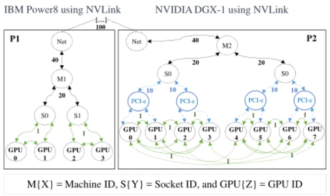
GPU topology based on the underlying hardware of a machine or a set of machines connected by a network. An example of how different physical GPU topologies are modeled is illustrated in Figure7, which shows the graph of Figure1’s topology. The physical graph can be understood as composed of multiple levels, where the first level is the network. Just after this level, there is the machine level, as represented by the vertexes M{X}, where X is the machine ID. The next level is the socket level and is represented as S{Y}, where Y accounts for the socket ID. Other levels can exist between the socket and the GPU, such as levels representing multiple PCI-e or NVLink switches. The last level represents the GPUs.

A GPU vertex can be directly connected to the socket vertex, to an intermediate vertex, and/or directly connected to other GPUs, which represents a direct NVLink connection between the GPUs. Consequently, some GPUs will have multiple paths to communicate. The path distance is given by the sum of the weight of the edges of the path. Since the weights are defined qualitatively, a higher level must have a larger weight to represent longer distances. For example, in Figure7each level right after the GPU level has weight 1, whilst at higher levels, such as the socket level, the edges have weight 20. Since the distances are qualitative, there are no con-straints on how the weights are defined, except that higher levels will have larger weights.

S0 S1 GPU 0 GPU 1 GPU 2 GPU 3 40 20 Net P1 M1

IBM Power8 using NVLink NVIDIA DGX-1 using NVLink

S0 GPU 0 GPU 1 GPU 2 GPU 3 20 20 Net P2 M2 1 1 PCI-e S0 GPU 4 GPU 5 GPU 6 GPU 7 40

PCI-e PCI-e PCI-e

1 1 1 1 1 10 10 10 10 […]

M{X} = Machine ID, S{Y} = Socket ID, and GPU{Z} = GPU ID

1 1 1 1

100

Figure 7: GPU physical topology graph.

4.2

Job Profile

The profile includes not only the job’s communication graph but also a performance model defining the level of interference the collocated jobs will suffer and cause. This model is created from experimentation using historical data. Two types of experiments can be defined. The first approach is injecting artificial load, using micro-benchmarks, onto the shared resources and measuring the interference, i.e. the impact on run-time of other collocated jobs. While this first approach can be highly accurate, analyze all possible combinations might be very costly. The second one is performing a combinatorial collocation of a set of known applications. Also, performance prediction for unknown jobs using the models from known applications can enlarge the range of the analysis. The previous workload executions can feed a prediction model, such as using decision tree [14,37] or statistical clustering [8,22,28]. Because of the cloud’s high variability, our model does not need to be optimal; high-quality decisions will be accurate enough.

4.3

Objective Function and Constraints

Our objective function focuses on minimizing the tasks communi-cation cost (tcc), external resource interference (Ib), and resource fragmentation (ωd). Formally, it can be defined as follows:

MIN αcctcc tw +αbI b Iw +αdω d ωw (1)

whereαcc+αb+αd =1. All parameterstcc,Ibandωd are nor-malized against the corresponding worst casetw,Iw andωw(i.e., the scenario with the lowest bandwidth, the highest interference, and the highest fragmentation). For the minimumtcc, we allocate GPUs as close as possible once all constraints are met. For the min-imumIb, we allocate GPUs with the lowest possible amount of bus sharing. For the minimumωd, we map GPUs from the most fragmented domains to increase the cluster utilization.

The constraints that we define in this paper are the resource capacity as the number of GPUs and the memory bandwidth. For-mally, all possible solutions must meet the inequality constraints defined astдpu ≤pдpuandtbw ≤pbw, wheretxandpxdenote the resource requirement of a given application and the available capacity of a given node for the resource typex, respectively. Other constraints can be added for different scenarios than the ones we show in our experiments.

Algorithm 1Topology-aware job placement algorithm A; //application’s job communication pattern graph

P; //physical topology graph

C; //communication cost array

Q; //jobs waiting queue sorted by their arrival time (oldest to newest)

functionscheduler(P)

whileT ruedo

whileavailableResources(P)andQ,∅do A←Q.pop()

P0_{←filterHostsByConstraints(A,P)}

s=DRB(A,P0_,C)

ifU(s)<A.minimal_utilityandpostpone=T ruethen postponed_list.add(A)

else

place(A,s)

Q.add(postponed_list)

sleep(interval) //wakeup after an event (e.g a job has finished)

4.4

Placement Algorithm

First, we define the premise and limitations. The algorithm behaves as a greedy algorithm since the assignment of a task to a physical GPU is never reconsidered. Hence, we perform a best-effort ap-proach to find the optimal solution. The algorithm preferentially places as many tasks as possible for a job in the same node. If a job wants to get all its tasks spread across different nodes in-stead, it needs to define anti-collocation policies for its tasks, and in response, they will be placed on different nodes. Also, if a job does not support multi-node, it must be defined with a single-node constraint in the profile. If a job cannot be placed, its placement is postponed to the next iteration of the scheduler. To avoid starvation and enforce fairness as much as possible, the job waiting queue is sorted by the job’s arrival time. Thus, the oldest jobs have priority to be placed.

We define two scheduling policies for the proposed algorithm. One policy is referred to TOPO-AWARE-P which allows out-of-order execution of jobs and postpone the placement that the job’s utility is lower than a threshold defined in the job’s profile. The other policy is the TOPO-AWARE, where the jobs are placed as soon as they arrive without consideration for the future jobs.

The placement process is formally defined as a functionψ() taking the job’s graphAand the physical topologyPasψ(A,P)and transforming them into the GPU listд. Where|A|is the number of requested GPUs,|P|is the number of available GPUs, and

д is the number of allocated GPUs to the job, being

д ≤ |P|.

Algorithm1outlines the placement process. It is a loop-based approach that each iteration attempts to place jobs while there are jobs in the waiting queueQand available resources. Otherwise, the scheduler sleeps until a job has finished or a time interval has expired. During each iteration, the scheduler takes a job fromQand filters the available nodes, eliminating the ones that do not satisfy the constraints (e.g. resources types, anti-affinity, etc.), creating the graphP0. Then, the functionDRB()is called to traverse the physical graphP0and define the GPU allocation. After that, if the utility of the solutionsdoes not satisfy the job’s requirements and the policy allows postponement, the job is added back to the waiting queue at the end of the iteration; otherwise, the placement is enforced.

The functionDRB(), outlined in Algorithm2, is based on the Hi-erarchical Static Mapping Dual Recursive Bi-partitioning algorithm

Algorithm 2Recursive Bi-Partitioning Mapping based in [12]

1: functionDRB(A,P,C) 2: if(|A|==0)then

3: returnnil//This partition is not a candidate 4: if(|P|==1)then

5: returnд←(P,A)//Map job’s task to physical GPU

6: (P0_,P1_{)=physicalGraphBiPartition(P)}

7: (A0_,C0_,A1_,C1_{)=jobGraphBiPartition(A,P}0_,P1_{, C)}

8: д0=DRB(A0_,P0_,C0₎

9: д1=DRB(A1_,P1_,C1₎

10: return(д0_+д1₎

Algorithm 3Utility-based job graph bi-partitioning

1: functionjobGraphBiPartition(A, P0_{, P}1_{, C)}

2: whileA,∅do

3: task←A.pop()

4: (P0.tc c_,P1_.tc c_{)←getCommCost(task,P}0_,P1_,C)

5: (P0.Ib,P1.Ib)←getInter(task,P0,P1,A.prof ile)

6: (P0_.ωd_,P1_.ωd_{)←getFragmentation(P}0_,P1_,A)

7: if(U(task,P0_)≥U(task,P1_{))and(constr aints)then}

8: A0.add(task) 9: else

10: A1.add(task) 11: returnA0_,P0_.tc c_,A1_,P1_.tc c

proposed by [12] and implemented by [34]. Its asymptotic complex-ity is defined asΘ(|E_A| ∗loд₂(|V_P|))[35], where in our case|E_A|is the number of edges from the job’s graph and|VP|is the number of a vertex from the physical graph.

More specifically, during each recursive iteration ofDRB() two other functions are called,physicalGraphBiPartition() to bi-partition the physical graph P, andjobGraphBiPartition() to bi-partition the job’s graph A. The recursion stops when A =∅, returning∅, or when Pyonly has one element, returning the map-ping pair (Ay, Py), wherey∈{0,1} partitions. The C parameter is an array that contains the communication cost of all GPUs, even the ones not into the sub-partition Py. C is used to calculate the communication cost between sub-partitions.

Similarly to the implementation of DRB() in [34], the physi-cal graph bi-partition is performed with the well-known Fiduccia Mattheyses algorithm [15] that minimizes the cut-sets in linear time. However, differently from [34], we do not only account the communication cost, but also the job’s preference using a utility function to bi-partition the job’s graph, as shown in the function jobGraphBiPartition() outlined in Algorithm3.

Algorithm3creates two sub-partitionsA0andA1, where each partition can have part or all the job’s tasks. Since the tasks inA0 will be placed inP0andA1inP1, the function evaluates for each task which sub-partition Py provides higher utility. Then, ifP1 gives better utility and has enough available resources, the task is added toA0. Otherwise, the task is added toA1.

For each task, Algorithm3evaluates each sub-partition via cal-culating the communication costt, the workload interferenceIand the resource fragmentationω, using the functionsgetCommCost(), getInter() andgetFragmentation(), respectively. Then, with those parameters the job’s utility is calculated using the utility function U, which can be defined as the convex function in Equation2.

U =(αcc1 t +αb 1 I +αd 1 ω) (2)

Next, we describe how theU parameters are calculated. The communication cost (t) is defined as the sum of the combinatorial shortest pathspbetween all GPUs within the solution as:

t = |P| X i=1 |P|−i X j=1 pi,j,wherei,j (3)

The level of interference (I) is measured using the job’s profile. As described in section4.2, the profile is composed by the completion time of the job running solo and running with other jobs (or with artificial loads). Therefore, the algorithm measures the average slowdown that the job suffers and causes in the currently running jobs. Thus, the average interference is calculated as follows:

I=

Prunninд_jobs+1

j=1 (solo_time(j)/collocation_time(j))

runninд_jobs+1 (4)

System fragmentation (ω) is the average fragmentation of all sockets, which is calculated as follows:

ω=

Psockets

i=1 (f reeGPU s(socketi)/totalGPU s(socketi))

sockets (5)

5

TOPOLOGY-AWARE SCHEDULER

EVALUATION

In this section, we present both a prototype implementation and a trace-driven simulation to evaluate the proposed topology-aware scheduler algorithm. The prototype evaluation was performed on a single machine with characteristics described in section3.1. The simulation evaluates the algorithm on a large scale cluster.

While the focus of this work is in learning workloads, any work-load can be submitted in the prototype. Also, there is no need to change how applications are implemented in order to use the scheduler. In the future, we plan to test the proposed algorithm in a cluster manager framework like Kubernetes [17] or Mesos [21], similar to the enhancements described in the related work [45].

5.1

Prototype Implementation

We implemented the prototype for the scheduler using C and Python. The program continuously loads JSON files containing the necessary information about the submitted jobs. To place a job, the system creates the job’s manifest, filling it with the information received from the JSON file, and uses that information to determine the placement of the job. If the algorithm decides to place the job, it enforces the decision of running the job on the given machine. Until the job finishes, the system keeps track of the execution of the job while collecting statistics including the ending time.

For the placement, the system captures various performance met-rics. The DRAM memory bandwidth is calculated using the Power8 performance counters described in [1], which are accessed using the library Perfmon2 [36]. To calculate the NVLink bandwidth (which is shown in most of the experiments), we access the NVIDIA CUDA driver API using the commandnvidia-smi nvlink -i $gpu_id that returns the transmitted bytes from each link. Then, the algo-rithm calculates the NVLink bandwidth usage of CPU-to-GPU or GPU-to-GPU communication based on their link connections.

For discovering the topology during the system startup, it ex-ecutes thenvidia-smi topo --matrixcommand1 to create a matrix of GPUs, and the commandnumactl --hardwareto in-clude socket distance and CPU locality in the model. For enforc-ing the decisions, before executenforc-ing any application, the system first defines the order of the GPU ID’s by exporting the parameter CUDA_DEVICE_ORDER=PCI_BUS_ID, and then, for each application, it exposes only the specified GPU list from the scheduler decisions using the parameterCUDA_VISIBLE_DEVICES=$gpu_list. For pre-venting performance variability related to NUMA remote memory access, the applications with only GPUs in the same socket are bound to the socket using the commandnumactl.

To feed the performance prediction model, the application pro-files are experimentally generated, defining the optimal resource al-location (best-performing) and some possible sub-optimal resource allocation (worst-performing) for both solo (when the job runs alone with no other jobs) and co-scheduled modes, as previously shown in Section3. The profile then contains the 95th percentile of the execution time from five executions of each workload within different scenarios. A simple, but effective performance prediction approach is then performed using the profiles, characterizing the workload slowdowns for various configurations; we plan to extend it with more robust statistical techniques in the future. Since Caffe framework is based on data-parallelism model, all GPUs perform similar work, and then, they have a similar amount of communi-cation between each other. Therefore, we define in the workload graph all GPUs communicating between each other with the same weight. However, for different batch sizes, different weights are used, ranging from 4 to 1, where 4 represents the smallest batch size and 1 the largest one.

5.2

Prototype Evaluation

We implement two well-known greedy approaches: First Come First Served (FCFS) with a FIFO queue, and Best Fit (BF) performing bin packing (i.e. allocating first the GPUs from highly used domains) and compare them to our proposed placement algorithm with the two scheduling policies: TOPO-AWARE and TOPO-AWARE-P. Fi-nally, we evaluate the prototype in a cloud environment, where jobs have varied GPU requirements: some needing a single GPU, some needing more than two GPUs, some requiring P2P to be fully satisfied, others needing multiple GPUs, but communication re-quirements are minimal. Additionally, as in a cloud environment, the jobs concurrently share any machine’s resources.

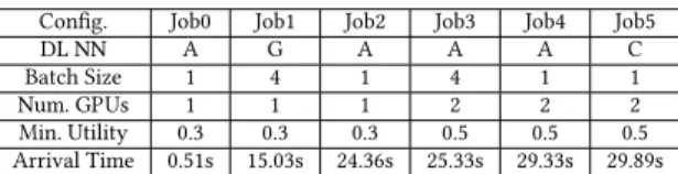
Config. Job0 Job1 Job2 Job3 Job4 Job5

DL NN A G A A A C

Batch Size 1 4 1 4 1 1

Num. GPUs 1 1 1 2 2 2

Min. Utility 0.3 0.3 0.3 0.5 0.5 0.5 Arrival Time 0.51s 15.03s 24.36s 25.33s 29.33s 29.89s

Table 1: A=AlexNet, C=CaffeRef, G=GoogLeNet

5.2.1 Description of the experiment.Our first experiment is a

simple, easy-to-verify scenario, with five jobs dynamically sharing the machine described in Section3.1. The workload configurations are summarized in Table1. Jobs’ arrival time follow a Poisson distribution configured withλ=10 (i.e. the arrival of ten jobs per

1_{The system targets only NVIDIA GPUs. But, for detecting GPUs from other vendors} the library HWLOC can be used.

0 1 2 3 GPU IDs (a) BF _J1 J0 J3 J2 J5 J4 0 48 96 144 192 240 288 336 384 432 480 528 0 16 32 48 GB/s GPU-CPU-GPU P2P 0 1 2 3 GPU IDs (b) FCFS _J1 J0 J3 J2 J5 J4 0 48 96 144 192 240 288 336 384 432 480 528 0 16 32 48 GB/s GPU-CPU-GPU_P2P 0 1 2 3 GPU IDs (c) TOPO-AWARE _J1 J0 J3 J2 J5 J4 0 48 96 144 192 240 288 336 384 432 480 528 0 16 32 48 GB/s GPU-CPU-GPU P2P 0 1 2 3 GPU IDs (d) TOPO-AWARE-P _J1 J0 J3 J2 J5 J4 0 48 96 144 192 240 288 336 384 432 480 528 Time (s) 0 16 32 48 GB/s GPU-CPU-GPU_P2P 3 4 1 5 0 2

Ordered jobs from worst to best-performing 0.0 0.2 0.4 0.6 0.8 Slo wdo wn (e) JOB’S QOS BF FCFS TOPO-AWARE TOPO-AWARE-P 5 4 3 1 0 2

Ordered jobs from worst to best-performing 0.0 0.2 0.4 0.6 0.8 Slo wdo wn (f) JOB’S QOS + WAITING TIME

Figure 8: [Prototype] Figures (a) to (d) present the time line of the placement decisions of each evaluated algorithm. A colored box can be on one or more GPU IDs, which represents the GPU allocation for a job. Figures (e) and (f) present the

slowdown is in comparison with the ideal scenario and the jobs are ordered from worst to best-performing.

0 1 2 3 GPU ID (a) BF _J1 J0 J3 J2 J5 J4 0 48 96 144 192 240 288 336 384 432 480 528 0.0 0.2 0.4 0.6 0.8 1.0 Utilit

y Mean Job Utility 0 1 2 3 GPU ID (b) FCFS _J1 J0 J3 J2 J5 J4 0 48 96 144 192 240 288 336 384 432 480 528 0.0 0.2 0.4 0.6 0.8 1.0 Utilit

y Mean Job Utility 0 1 2 3 GPU ID (c) TOPO-AWARE _J1 J0 J3 J2 J5 J4 0 48 96 144 192 240 288 336 384 432 480 528 0.0 0.2 0.4 0.6 0.8 1.0 Utilit

y Mean Job Utility

0 1 2 3 GPU ID (d) TOPO-AWARE-P _J1 J0 J3 J2 J5 J4 0 _{48 96 144 192 240 288 336 384 432 480 528} Time (s) 0.0 0.2 0.4 0.6 0.8 1.0 Utilit

y Mean Job Utility

1 4 3 5 0 2

Ordered jobs from worst to best-performing 0.0 0.2 0.4 0.6 0.8 Slo wdo wn (e) JOB’S QOS BF FCFS TOPO-AWARE TOPO-AWARE-P 5 4 3 1 0 2

Ordered jobs from worst to best-performing 0.0 0.2 0.4 0.6 0.8 Slo wdo wn (f) JOB’S QOS + WAITING TIME

Figure 9: [Simulation] Behavioral description of the simulation performing a similar experiment to that shown for the prototype in Figure8.

minute), except the Job 0 which arrives at timet=0.51sto introduce the initial load in the system. We set equal weights (0.33) to the parameters of the utility function in Equation2to provide equal consideration for communication cost and resource interference and fragmentation. Small batch sizes represent a reliable example of NNs that requires high GPU communication (especially for NNs using model-parallelism). Hence, we conduct this experiment using small batch sizes.

5.2.2 Prototype experimental results.The results are shown in

Figure8. In the beginning, only Job 0 is being placed. And since it requires only one GPU and there is no other job to cause interfer-ence, any placement decision fully satisfies its requirements. At the 15thsecond, Job 1 arrives and the profile indicates that it suffers in-terference from Job 0. Thus, the overall system utility will be lower

if Job 0 and Job 1 are collocated in the same CPU socket. On the other hand, TOPO-AWARE-P prevents the undesirable collocation; it places Job 1 on a different socket than Job 0. When Job 3 arrives, it cannot be placed since it requires more GPUs than available. So Job 3 is only placed after Job 0 has finished,≈70thsecond. However, at this point resource availability is non-uniform: the available GPUs are in different sockets.

Here is where the TOPO-AWARE-P differs from the other ap-proaches. If Job 3 receives the two free GPUs, one from each of the sockets, this will result in cross-socket communication over the CPU bus and results in lower performance. For this reason, the TOPO-AWARE-P delays the job placement to until it can allo-cate co-loallo-cated GPUs, that is, when these GPUs become available. Any job with the utility lower than a threshold defined in the job’s

profile will have the placement postponed to the next scheduler iteration. As a result, the TOPO-AWARE-P performs better in exe-cution time than the others, as shown in Figure8(d) vs Figures8

(a)-(c). For example, Job 3 had the completion time as≈120s for the scenario with the TOPO-AWARE-P (Figure8(d)), and≈240s with the other algorithms. Note that the performance improvement is mainly related to enabling P2P over the NVLink interface to Job 3. Only the TOPO-AWARE-P provides P2P for jobs as shown in Figure

8(d), in all the other scenarios the GPU communication is routed through the processor’s memory, which leads to higher latency, and lower bandwidth because of additional memory copies and potential contention of the shared bus.

The quality of the placement is highlighted in Figure8(e) and (f). Both figures show the job’s slowdown compared to the ideal scenario, where the job has the fastest execution time. Also, both figures sort the jobs from worst to best-performing. While Figure

8(e) focuses on showing the job slowdown strictly related to the placement decision, Figure8(f) shows the slowdown also consider-ing the waitconsider-ing time in the scheduler’s queue. The results indicate that TOPO-AWARE-P is the most efficient algorithm. For instance, with TOPO-AWARE-P, jobs 1, 3, and 4 have no slowdown com-pared to the best-performing scenario, while these same jobs suffer ≈50% slowdown when the other algorithms are making placement decisions, as shown in Figure8(e).

Intuitively, delaying jobs gives the impression that the queue waiting time might end up being longer. However, the results sur-prisingly show that TOPO-AWARE-P has a lower waiting time for some jobs than other algorithms, as shown in Figure8(f). This hap-pens because having better knowledge of the requirements enables the scheduler to prevent performance interference, and then some jobs will execute faster, opening space to place other jobs sooner. This can also be seen in the cumulative execution time of the algo-rithms. BF finishes in≈461.7s, FCFS in≈456.2s, TOPO-AWARE in ≈454.2s, and TOPO-AWARE-P≈356.9s. Hence, TOPO-AWARE-P affords a speedup of≈1.30x,≈1.28x, and≈1.27x, respectively.

5.3

Trace-Driven Simulation

Based on the logs from the prototype described in Section5, we developed a trace-driven simulation to evaluate the scheduling algorithm in large shared clusters. In this section, we first describe the main characteristics and configuration of the simulation. And second, we validate the simulation and perform experiments with a larger number of jobs and machines.

To evaluate the scalability, the proposed algorithm was executed to handle trace-driven simulated data at different scales of the sys-tem. The traces are generated by performing multiple experiments on the previously described prototype. Afterward, the trace files are parsed and transformed into a format compatible with the simulator, creating application and resource usage profiles. For generating the workloads, a Poisson distribution with arrival rateλ=10 is used. To create the job’s configuration, we used a Binomial distribution generating integer values between 0 and 3 to define the batch size, where 0=tiny, 1=small, 2=medium, and 3=big. And also a Binomial distribution generating integer values between 0 and 2 to determine the NN type, where 0=AlexNet, 1=CaffeRef, and 2=GoogLeNet. Ad-ditionally, all simulated machines are homogeneous and follow the

hardware topology described in Section3.1. All the jobs can run in the machines when there are enough resources.

5.4

Validation of The Simulation

We validate the reliability of the simulation system by comparing it with the same scenario as in the prototype experiments in Section5. The simulation results are shown in Figure9. The algorithms behave very similarly in both prototype and the simulation, despite some expected small differences, which are acceptable when considering the standard deviations.

5.5

Large-Scale Cluster Simulation and Results

To verify the behavior of the proposed algorithm in a large-scale environment, we use the trace-driven simulation in two different scenarios as follows.

Ordered jobs from worst to best 0.00 0.25 0.50 0.75 Slo wdo wn (a) JOB’S QOS BF FCFS TOPO-AWARE TOPO-AWARE-P

Ordered jobs from worst to best 0.00 0.25 0.50 0.75 Slo wdo wn (b) JOB’S QOS + WAITING TIME

Figure 10: Scenario 1: 100 jobs and 5 machines. Job’s slowdown relative to the best performing configuration.

5.5.1 Scenario 1: 100 jobs and 5 machines.We start the first

experiment with few machines and jobs. The results in Figure10(a) show that the TOPO-AWARE-P policy performs slightly better than the other; it does not violate the job’s SLO. The other strategies introduce similar slowdowns in general, except FCFS that adds slowdown in more jobs.

The performance difference between the placement strategies is more evident when analyzing the waiting time of jobs in the scheduling queue, as illustrated in Figure10(b). Both TOPO-AWARE and TOPO-AWARE-P clearly outperform the greedy algorithms.

The lower performance of the greedy algorithms is explained by the fact that a sub-optimal placement decision can also limit the possible placements of other jobs. If a machine is left with only one GPU and the waiting jobs require more GPUs, the jobs must wait to be placed until enough resource becomes available. While less expressive, TOPO-AWARE-P performs better than only TOPO-AWARE. The second still presents slowdown in some jobs, and the former does not, since it allows out-of-order execution of jobs. TOPO-AWARE-P results in better performance because it does not schedule jobs to resources that do not fully satisfy its QoS.

Ordered jobs from worst to best 0.0 0.2 0.4 0.6 0.8 Slo wdo wn (a) JOB’S QOS FCFS BF TOPO-AWARE TOPO-AWARE-P

Ordered jobs from worst to best 0.0 0.2 0.4 0.6 0.8 Slo wdo wn (b)

JOB’S QOS + WAITING TIME

Figure 11: Scenario 2: 10k jobs and 1k machines. Job’s slowdown relative to the best performing configuration.

5.5.2 Scenario 2: 10k jobs and 1k machines. The results in Fig-ure11show that the FCFS algorithm has the worst performance, followed by BF. In summary, the new algorithm significantly and consistently outperforms the greedy algorithms in achieving the least slowdown and in minimizing the waiting time. The new al-gorithm’s ability to achieve this is mainly due to its utility-based heuristics and the strategy that does not place jobs when the place-ment is not efficient from a communication perspective.

5.5.3 Overhead. The average time that the algorithms spend

when evaluating the placement decision in scenario 2 is≈3s for TOPO-AWARE and TOPO-AWARE-P, while for FCFS and BF it is ≈0.45s and≈0.44s respectively. Although the proposed algorithm has higher overhead, 3 seconds on average is fast enough for sched-uling learning workload on a cluster with high demands.

The proposed algorithm has a higher execution time than the greedy ones mainly because it requires more computation to pro-vide a better decision. Note that in the worst case, our proposed algorithm will evaluateΘ(|V_P|)∗Θ(|E_A| ∗loд₂(|V_P|)), where the firstΘrepresents the host filtering phase and the second represents the phase to make the placement decision. Where the|E_A|is the number of edges from the job’s graph and|VP|is the number of a vertex from the physical graph. The other greedy algorithms have the asymptotic complexity asΘ(|E_A|+|V_P|)since every machine will be explored in the worst case.

6

RELATED WORK

Communication cost.Kindratenko et. al. [26] proposed a CUDA wrapper that works in sync with Torque batch system. The wrapper overrides some CUDA device management API calls to expose GPUs to users, taking into account the GPUs distance to provide best-efforts on minimizing the communication cost. Faraji et. al. [13] propose a topology-aware GPU selection scheme to assign GPU devices to MPI processes based on the GPU-to-GPU communication pattern and the physical characteristics of a multi-GPU machine. With profile information from the MPI application, it allocates GPUs performing a graph mapping algorithm using the SCOTCH library. While those efforts effectively minimize the communication cost, they do not consider the potential performance interference from co-scheduled jobs. In this paper, different from the above-related work, we further analyze and mitigate performance problem, and leverage P2P communication for multi-GPU based learning workloads in a co-scheduled environment.

Workload Collocation.Several papers investigate the perfor-mance of co-running CPU-based workload [41], [20], [24], [27], [11], and GPU-based workloads [25] and [44]. In addition, several papers proposed scheduling algorithms to avoid problematic collocation within the same machine [33], [9], [32], [7], or with best-efforts on minimize the CPU resources interference performing low-level resource partitioning [38], [4], [19], and [29]. While those papers describe the performance bottlenecks for CPU-only application and/or providing best-efforts on mitigating workload interference, they neither directly show the performance constraints of mixing multiple GPU-based learning workloads, nor do they propose a GPU-topology-aware scheduling algorithm.

Mapping Algorithm.Several researchers have been proposing heuristics for graph mapping such as graph contraction [5], and

graph embedding [39], [43], [30], [40] and recursive bi-partitioning algorithm [12] that has been implemented in the software package SCOTCH [34]. While those methods have been proved to be an effective approach, most of them are contiguous with static alloca-tion approaches leading to resource fragmentaalloca-tion and focus only minimizing the communication cost, not considering the other char-acteristics, such as the resource sharing interference. In contrast, our work considers a utility function during the mapping phase, which captures the application’s preference on different scenarios, and therefore, preventing SLO violations.

7

CONCLUSIONS

Multi-GPU applications are becoming popular because they can deliver performance improvements and increased energy efficiency. But at the same time, they present new challenges as they usually require inter-GPU communications. Such communications can take place directly between devices (with P2P) or may need to be routed through the processors’ main memory, depending on the system topology and the resource allocations for the existing jobs.

In this paper, we presented a new topology-aware placement algorithm for scheduling workloads in modern multi-GPU systems. The foundation of this approach is based on the use of a new graph mapping algorithm built from application objectives and the system topology. Applications can express their performance objectives as SLOs that are later translated into abstract utility functions to drive the placement decisions. The algorithm has been validated through the construction of a real prototype on top of an IBM Power8 system enabled with 4 NVIDIA Tesla P100 cards, as well as through large-scale simulations.

Our experiments show that our algorithm effectively reduces the communication cost while preventing interference related to resource contention, mainly for the scheduling policy that allows postponing the placement of unsatisfied jobs. In particular, with this policy, the performance impact of minimizing the GPU commu-nication cost and avoiding interference reflects in a speedup of up to≈1.30x in the cumulative execution time, and no SLO violations. Finally, a trace-driven simulation of a large-scale cluster reveals that compared with greed approaches our algorithm produces solutions that satisfy more jobs, minimizes the SLO violations and improves the job’s execution time even in a heavily loaded scenario.

In the future, we plan to extend this work to transparently scale learning applications to multiple disaggregated GPUs across the cluster and test the implementation of our algorithm in popular resource management systems such as Kubernetes and Mesos.

ACKNOWLEDGMENTS

This project is supported by the IBM/BSC Technology Center for Super-computing collaboration agreement. It has also received funding from the European Research Council (ERC) under the European Union’s Horizon 2020 research and innovation programme (grant agreement No 639595). It is also partially supported by the Ministry of Economy of Spain under contract TIN2015-65316-P and Generalitat de Catalunya under contract 2014SGR1051, by the ICREA Academia program, and by the BSC-CNS Severo Ochoa pro-gram (SEV-2015-0493). We thank our IBM Research colleagues Alaa Youssef and Asser Tantawi for the valuable discussions. We also thank SC17 com-mittee member Blair Bethwaite of Monash University for his constructive feedback on the earlier drafts of this paper.

REFERENCES

[1] Andrew V. Adinetz, Paul F. Baumeister, Hans Böttiger, Thorsten Hater, Thilo Maurer, Dirk Pleiter, Wolfram Schenck, and Sebastiano Fabio Schifano. 2015. Per-formance Evaluation of Scientific Applications on POWER8. Springer International Publishing, Cham, 24–45. DOI:http://dx.doi.org/10.1007/978-3-319-17248-4_2 [2] Amazon. 2017. Amazon Machine Learning. (2017).https://aws.amazon.com/

machine-learning/

[3] Soheil Bahrampour, Naveen Ramakrishnan, Lukas Schott, and Mohak Shah. 2015. Comparative Study of Caffe, Neon, Theano, and Torch for Deep Learning.CoRR

abs/1511.06435 (2015).http://arxiv.org/abs/1511.06435

[4] Gaurav Banga, Peter Druschel, and Jeffrey C. Mogul. 1999. Resource Containers: A New Facility for Resource Management in Server Systems. InProceedings of the Third Symposium on Operating Systems Design and Implementation (OSDI ’99). USENIX Association, Berkeley, CA, USA, 45–58.http://dl.acm.org/citation. cfm?id=296806.296810

[5] Francine Berman and Lawrence Snyder. 1987. On Mapping Parallel Algorithms into Parallel Architectures.J. Parallel Distrib. Comput.4, 5 (Oct. 1987), 439–458. DOI:http://dx.doi.org/10.1016/0743-7315(87)90018-9

[6] Léon Bottou, Frank E. Curtis, and Jorge Nocedal. 2016. Optimization Methods for Large-Scale Machine Learning.CoRRabs/1606.04838 (2016).http://arxiv.org/ abs/1606.04838

[7] Brendan Burns, Brian Grant, David Oppenheimer, Eric Brewer, and John Wilkes. 2016. Borg, Omega, and Kubernetes.ACM Queue14 (2016), 70–93.

[8] Christina Delimitrou and Christos Kozyrakis. 2014. Quasar: Resource-efficient and QoS-aware Cluster Management. InProceedings of the 19th International Conference on Architectural Support for Programming Languages and Operating Systems (ASPLOS ’14). ACM, New York, NY, USA, 127–144.DOI:http://dx.doi. org/10.1145/2541940.2541941

[9] Christina Delimitrou and Christos Kozyrakis. 2014. Quasar: Resource-efficient and QoS-aware Cluster Management. InProceedings of the 19th International Conference on Architectural Support for Programming Languages and Operating Systems (ASPLOS ’14). ACM, New York, NY, USA, 127–144.DOI:http://dx.doi. org/10.1145/2541940.2541941

[10] Chris Edwards. 2015. Growing Pains for Deep Learning.Commun. ACM58, 7 (jun 2015), 14–16.DOI:http://dx.doi.org/10.1145/2771283

[11] Yaakoub El-Khamra, Hyunjoo Kim, Shantenu Jha, and Manish Parashar. 2010. Exploring the Performance Fluctuations of HPC Workloads on Clouds. In Pro-ceedings of the 2010 IEEE Second International Conference on Cloud Computing Technology and Science (CLOUDCOM ’10). IEEE Computer Society, Washington, DC, USA, 383–387. DOI:http://dx.doi.org/10.1109/CloudCom.2010.84 [12] F. Ercal, J. Ramanujam, and P. Sadayappan. 1988. Task Allocation Onto a

Hyper-cube by Recursive Mincut Bipartitioning. InProceedings of the Third Conference on Hypercube Concurrent Computers and Applications: Architecture, Software, Computer Systems, and General Issues - Volume 1 (C3P). ACM, New York, NY, USA, 210–221. DOI:http://dx.doi.org/10.1145/62297.62323

[13] Iman Faraji, Seyed Hessam Mirsadeghi, and Ahmad Afsahi. 2016. Topology-Aware GPU Selection on Multi-GPU Nodes. In2016 IEEE International Parallel and Distributed Processing Symposium Workshops, IPDPS Workshops 2016, Chicago, IL, USA, May 23-27, 2016. 712–720.DOI:http://dx.doi.org/10.1109/IPDPSW.2016.44 [14] Damon Fenacci, Björn Franke, and John Thomson. 2010. Workload

Characteri-zation Supporting the Development of Domain-specific Compiler OptimiCharacteri-zations Using Decision Trees for Data Mining. InProceedings of the 13th International Workshop on Software &#38; Compilers for Embedded Systems (SCOPES ’10). ACM, New York, NY, USA, Article 5, 10 pages. DOI:http://dx.doi.org/10.1145/1811212. 1811219

[15] C. M. Fiduccia and R. M. Mattheyses. 1982. A Linear-time Heuristic for Improving Network Partitions. InProceedings of the 19th Design Automation Conference (DAC ’82). IEEE Press, Piscataway, NJ, USA, 175–181.

[16] Google. 2017. Google Cloud Prediction API Documentation. (2017). https: //cloud.google.com/prediction/docs/

[17] Google. 2017. Kubernetes. (2017). https://github.com/googlecloudplatform/ kubernetesAccessed in: 21-January-2015.

[18] Samuel Greengard. 2016. GPUs Reshape Computing.Commun. ACM59, 9 (Aug. 2016), 14–16. DOI:http://dx.doi.org/10.1145/2967979

[19] Akhila Gundu, Gita Sreekumar, Ali Shafiee, Seth Pugsley, Hardik Jain, Rajeev Balasubramonian, and Mohit Tiwari. 2014. Memory Bandwidth Reservation in the Cloud to Avoid Information Leakage in the Memory Controller. InProceedings of the Third Workshop on Hardware and Architectural Support for Security and Privacy (HASP ’14). ACM, New York, NY, USA, 11:1–11:5.DOI:http://dx.doi.org/ 10.1145/2611765.2611776

[20] Anshul Gupta. 2010.An Evaluation of Parallel Graph Partitioning and Ordering Softwares on a Massively Parallel Computer. IBM T. J. Watson Research Center. All pages.

[21] Benjamin Hindman, Andy Konwinski, Matei Zaharia, Ali Ghodsi, Anthony D. Joseph, Randy Katz, Scott Shenker, and Ion Stoica. 2011. Mesos: A Platform for Fine-grained Resource Sharing in the Data Center. InProceedings of the 8th USENIX Conference on Networked Systems Design and Implementation (NSDI’11).

USENIX Association, Berkeley, CA, USA, 295–308.http://dl.acm.org/citation. cfm?id=1972457.1972488

[22] Kenneth Hoste, Aashish Phansalkar, Lieven Eeckhout, Andy Georges, Lizy K. John, and Koen De Bosschere. 2006. Performance Prediction Based on Inherent Program Similarity. InProceedings of the 15th International Conference on Parallel Architectures and Compilation Techniques (PACT ’06). ACM, New York, NY, USA, 114–122. DOI:http://dx.doi.org/10.1145/1152154.1152174

[23] IBM. 2017. Go beyond artificial intelligence with Watson. (2017).https://www. ibm.com/watson/

[24] Alexandru Iosup, Nezih Yigitbasi, and Dick Epema. 2011. On the Performance Variability of Production Cloud Services. InProceedings of the 2011 11th IEEE/ACM International Symposium on Cluster, Cloud and Grid Computing (CCGRID ’11). IEEE Computer Society, Washington, DC, USA, 104–113.DOI:http://dx.doi.org/ 10.1109/CCGrid.2011.22

[25] Onur Kayiran, Nachiappan Chidambaram Nachiappan, Adwait Jog, Rachata Ausavarungnirun, Mahmut T. Kandemir, Gabriel H. Loh, Onur Mutlu, and Chita R. Das. 2014. Managing GPU Concurrency in Heterogeneous Architectures. In

Proceedings of the 47th Annual IEEE/ACM International Symposium on Microar-chitecture (MICRO-47). IEEE Computer Society, Washington, DC, USA, 114–126. DOI:http://dx.doi.org/10.1109/MICRO.2014.62

[26] V. V. Kindratenko, J. J. Enos, G. Shi, M. T. Showerman, G. W. Arnold, J. E. Stone, J. C. Phillips, and W. m. Hwu. 2009. GPU clusters for high-performance computing. In2009 IEEE International Conference on Cluster Computing and Workshops. 1–8. DOI:http://dx.doi.org/10.1109/CLUSTR.2009.5289128

[27] Philipp Leitner and Juergen Cito. 2014. Patterns in the Chaos - a Study of Performance Variation and Predictability in Public IaaS Clouds.arXiv:1411.2429 [cs](Nov. 2014). arXiv: 1411.2429.

[28] David Lo, Liqun Cheng, Rama Govindaraju, Parthasarathy Ranganathan, and Christos Kozyrakis. 2015. Heracles: Improving Resource Efficiency at Scale. In

Proceedings of the 42Nd Annual International Symposium on Computer Architecture (ISCA ’15). ACM, New York, NY, USA, 450–462.DOI:http://dx.doi.org/10.1145/ 2749469.2749475

[29] David Lo, Liqun Cheng, Rama Govindaraju, Parthasarathy Ranganathan, and Christos Kozyrakis. 2016. Improving Resource Efficiency at Scale with Heracles.

ACM Trans. Comput. Syst.34, 2, Article 6 (May 2016), 33 pages.DOI:http://dx. doi.org/10.1145/2882783

[30] Virginia Lo, Kurt J. Windisch, Wanqian Liu, and Bill Nitzberg. 1997. Non-contiguous Processor Allocation Algorithms for Mesh-Connected Multicom-puters. IEEE Trans. Parallel Distrib. Syst.8, 7 (July 1997), 712–726. DOI: http://dx.doi.org/10.1109/71.598346

[31] Microsoft. 2017. Project Oxford - Cognitive Services APIs. (2017).https://www. microsoft.com/cognitive-services/

[32] Ripal Nathuji, Aman Kansal, and Alireza Ghaffarkhah. 2010. Q-clouds: Managing Performance Interference Effects for QoS-aware Clouds. InProceedings of the 5th European Conference on Computer Systems (EuroSys ’10). ACM, New York, NY, USA, 237–250.DOI:http://dx.doi.org/10.1145/1755913.1755938

[33] Dejan Novaković, Nedeljko Vasić, Stanko Novaković, Dejan Kostić, and Ricardo Bianchini. 2013. DeepDive: Transparently Identifying and Managing Perfor-mance Interference in Virtualized Environments. InPresented as part of the 2013 USENIX Annual Technical Conference (USENIX ATC 13). USENIX, San Jose, CA. [34] FranÃğois Pellegrini. 2001. Scotch and libScotch 3.4 User’s Guide. (2001). [35] FranÃğois Pellegrini and Jean Roman. 1996.Experimental Analysis of the Dual

Recursive Bipartitioning Algorithm for Static Mapping. Technical Report. TR 1038-96, LaBRI, URA CNRS 1304, Univ. Bordeaux I.

[36] Perfmon2. 2016. Improving performance monitoring on Linux. (2016).http: //perfmon2.sourceforge.net

[37] J. R. Quinlan. 1986. Induction of Decision Trees.Mach. Learn.1, 1 (March 1986), 81–106.DOI:http://dx.doi.org/10.1023/A:1022643204877

[38] Moinuddin K. Qureshi and Yale N. Patt. 2006. Utility-Based Cache Partitioning: A Low-Overhead, High-Performance, Runtime Mechanism to Partition Shared Caches. InProceedings of the 39th Annual IEEE/ACM International Symposium on Microarchitecture (MICRO 39). IEEE Computer Society, Washington, DC, USA, 423–432. DOI:http://dx.doi.org/10.1109/MICRO.2006.49

[39] Roberto Tamassia. 1987. On Embedding a Graph in the Grid with the Minimum Number of Bends.SIAM J. Comput.16, 3 (June 1987), 421–444. DOI:http://dx. doi.org/10.1137/0216030

[40] Ozan Tuncer, Vitus J. Leung, and Ayse K. Coskun. 2015. PaCMap: Topology Map-ping of Unstructured Communication Patterns Onto Non-contiguous Allocations. InProceedings of the 29th ACM on International Conference on Supercomputing (ICS ’15). ACM, New York, NY, USA, 37–46.DOI:http://dx.doi.org/10.1145/2751205.

2751225

[41] Akshat Verma, Puneet Ahuja, and Anindya Neogi. 2008. Power-aware Dynamic Placement of HPC Applications. InProceedings of the 22Nd Annual International Conference on Supercomputing (ICS ’08). ACM, New York, NY, USA, 175–184. DOI:http://dx.doi.org/10.1145/1375527.1375555

[42] Linnan Wang, Wei Wu, George Bosilca, Richard W. Vuduc, and Zenglin Xu. 2016. Efficient Communications in Training Large Scale Neural Networks.CoRR

abs/1611.04255 (2016).http://arxiv.org/abs/1611.04255

[43] Kurt Windisch, Virginia Lo, and Bella Bose. 1995. Contiguous And Non-Contiguous Processor Allocation Algorithms For K-Ary n-Cubes.IEEE Transac-tions on Parallel and Distributed Systems8 (1995), 712–726.

[44] J. Wu and B. Hong. 2013. Collocating CPU-only Jobs with GPU-assisted Jobs on GPU-assisted HPC. In2013 13th IEEE/ACM International Symposium on Cluster, Cloud, and Grid Computing.DOI:http://dx.doi.org/10.1109/CCGrid.2013.19 [45] Seetharami R. Seelam Yu Bo Li, IBM Research. 2017. Speeding up Deep

Learn-ing Services: When GPUs meet Container Clouds, NVIDIA GPU Technology Conference. (2017).http://on-demand.gputechconf.com/gtc/2017/presentation/ s7258-seetharami-seelam-speed-up-deep-learning-service.pdfAccessed in: 5-August-2017.

A

APPENDIX

A.1

Description

(1) Check-list (artifact meta information):

• Algorithm: the paper describes in details the utility-based algorithm that performs a bipartite graph match-ing algorithm and used for schedulmatch-ing Deep Learnmatch-ing jobs in a prototype and a simulation.

• Program: the experiments use only open-source tools and benchmarks.

• Compilation: The application that collects hardware counters also requires to be compiled, but, apart from that, there is no special compilation needed. • Binary: Caffe framework and the perfmon2 library are

compiled from source. All the source code is available on-line.

• Run-time: all experiments are run on the Linux oper-ating system running with and without enabling the simulation mode in the system.

• Hardware: all experiments are run on the Power8 system further detailed in the paper.

• Run-time state: the system is idle and only running our experiments.

• Execution: from the shell command line as described in this appendix.

• Output: the results are shown in the paper as graphs. • Experiment workflow: outlined in this appendix. (2) How delivered: The system implemented is delivered as

source code in Github: http://github.com/HiEST/gpu-topo-aware.

(3) Hardware dependencies: The system relies on NVIDIA GPUs and commands for topology discovering and metrics collection. Some PMU events code are specific to Power8 architecture, whose documentation is public available in IBM official website. Additionally, it is necessary that P2P capabilities are enabled in the BIOS.

(4) Software dependencies: Caffe is public available in

https://github.com/BVLC/caffeand the library perfmon2 in

http://perfmon2.sourceforge.net/. All the benchmarks used for the experiments are available in the Caffe source code and requires no modification except from changing the training batch size.

A.2

Installation

There is no special installation of the system, except only for the previous dependencies described before.

A.3

Experiment workflow

This section describes how to configure the system and the experi-ment workflow.

The system can run in the simulation mode or as a real prototype based on predefined configuration fileetc/configs/sys-config. ini, changing the parameter simulation to True or False. When the simulation is false, the system will run jobs accordingly to user-defined bash script file (workload manifest), which receives the jobs and runtime (e.g. GPU ids) information and translate it to a command to execute a Caffe instance.

There is also a workload generator, which receives as parameters the arrival rate and probabilities of batch size, the amount of GPUs and workload type as described in the paper.

Each scheduler algorithm also has a configuration file etc/configs/algo-name-config.ini, which must be provide from at least one algorithm. If many are provided, the system will execute multiples runs configured with different schedule algo-rithm.

After providing the needed configuration files and workload manifests, to execute the system is only required to run the main file as “python main.py”.

Samples of all configuration files and workload manifest are provided in the source code.

The figures generated for the experiment section in the paper were provided from the scripts in thesrc/plot/*.

A.4

Experiment customization