Working Paper/Document de travail
2008-17
Policy Coordination in an
International Payment System
Bank of Canada Working Paper 2008-17
May 2008
Policy Coordination in an
International Payment System
by
James T. E. Chapman
Department of Banking Operations Bank of Canada
Ottawa, Ontario, Canada K1A 0G9 [email protected]
Bank of Canada working papers are theoretical or empirical works-in-progress on subjects in economics and finance. The views expressed in this paper are those of the author.
Acknowledgements
I would like to thank Stephen D. Williamson, Charles H. Whiteman, Paula Hernández-Verme, Hiroshi Fujiki, Ben Fung, and Miguel Molico for helpful comments and suggestions. I would also like to thank seminar participants at the University of Iowa Macro Lunch, 2005 Midwest Macroeconomics Meetings, the 2005 Canadian Economics Association meeting, The Economics of Payments II conference, the Bank of Canada, the University of Ottawa, and the Federal Reserve Board of Governors for comments and discussion. This paper originally circulated under the title “Policy in International Payment Systems with a Timing Friction.”
Abstract
Given the increasing interdependence of both financial systems and attendant payment and settlement systems a vital question is what form should optimal policy take when there are two connected payment systems with separate regulators.
In this paper I show that two central banks operating in a non-cooperative way will not have an incentive to achieve the optimal allocation of goods. I further show that this non-cooperative outcome will be supported by a zero intraday interest rate and constant fixed exchange rate. This is in contrast to recent research; which has shown that domestically a zero intraday interest rate will achieve a social optimum and that the central bank has an incentive to achieve it.
JEL classification: E58, E42, F31, F33
Bank classification: Payment, clearing, and settlement systems; Exchange rate regimes
Résumé
Étant donné l’interdépendance croissante des systèmes financiers et des systèmes de paiement et de règlement qu’ils englobent, il est primordial de déterminer quelle est la politique monétaire optimale lorsque deux systèmes de paiement interconnectés sont assujettis à la surveillance d’autorités distinctes.
L’auteur montre que, dans un cadre non coopératif, les deux banques centrales n’ont pas intérêt à répartir les biens de façon optimale. Il montre également qu’une répartition non optimale est compatible avec un taux d’intérêt intrajournalier nul et un taux de change fixe. Ce résultat est contraire aux conclusions de travaux récents voulant que le maintien du taux d’intérêt intrajournalier à zéro garantisse la réalisation d’un équilibre socialement optimal et que la banque centrale soit incitée à atteindre cet équilibre.
Classification JEL : E58, E42, F31, F33
Classification de la Banque : Régimes de taux de change; Systèmes de paiement, de compensation et de règlement
1
Introduction
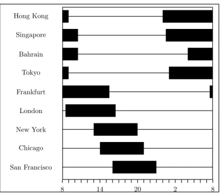
In this paper, I characterize the optimal policy in a two settlement-system world and then determine whether this policy can be implemented by two cen-tral banks acting non-cooperatively. Recent work by Hern´andez-Verme (2005), Fujiki (2003), and Fujiki (2006) has extended the payment literature to investi-gate the effects that payment frictions have in an international setting between two countries under the gold standard. This research bypasses the question of whether the socially optimal policy between two countries is achievable in a non-cooperative setting, focusing instead on issues related to the gold standard. The increasing integration of financial markets makes optimal policy among different large value settlement systems particularly relevant today due to in-terdependencies between systems. Major financial institutions are scattered around the globe in several different time zones. In addition, trading activ-ity, as well as the settlement of trades, may not be uniform during the time a market is open. Because of this geographic dispersion, the services of a given settlement system (e.g., Fedwire) might only be available at certain times of the day. Figure 1 (adapted from Melvin (1995, p.10–11)) illustrates the large variation in the trading hours of major financial centers. The foreign exchange (FX) market is dispersed among these many countries. In addition, the hours of operation for these different countries vary tremendously: some countries might be settling transactions (e.g., England) when it is still early in the trading day in other countries (e.g., United States).
Unlike previous literature dealing with international payments, I focus specif-ically on optimal policy between two countries which are identical in every re-spect except that they are located in different time zones. This difference in trading days between countries allows foreign exchange policy to be indepen-dent from liquidity provision in the central market.
What effect does this dispersion of trading hours have on intraday foreign exchange rates and intraday interest rates? Is it optimal for a central bank to set the intraday interest rate equal to zero? Previous research, such as Mar-tin (2004), has suggested that a zero interest-rate is optimal policy in a single payment system. Should a central bank set it to smooth the “lumpiness” in trading activity? More importantly, can two central banks, working indepen-dently, achieve an efficient allocation?
To answer these questions, I construct a model—developed in sections 2 through 5 —in which agents in two countries are unable to coordinate domestic and international payments because each country is open for trade at different
Hong Kong Singapore Bahrain Tokyo Frankfurt London New York Chicago San Francisco 8 14 20 2 8
Figure 1: Trading hours (GMT) for different major currency exchanges. times. The model I construct is based on Freeman (1996) and is similar to Fujiki (2003) and Fujiki (2006). In section 6, I investigate the equilibrium of these economies without intervention, while in section 7, I define the optimal consumption sequence as that which would have been chosen by a benevolent social planner. I then go on to analyze optimal monetary policy under a single authority (section 8) and under two authorities (section 8.1).
I find that while the optimal allocation is obtainable by the regime with two central banks, the two central banks do not have an incentive to achieve the social optimum. This is in contrast to the results of Fujiki (2003). While Fujiki (2003) finds that a fixed exchange rate and active intervention increases welfare I find that the policies implemented by the two central banks do not attain the social planner’s allocation when they behave non-cooperatively.
In addition, the Nash equilibrium policy that the two central banks imple-ment in a stationary equilibrium involves setting the intraday interest rate in the domestic settlement markets equal to zero; this is in contrast to Martin (2004) who finds that a zero intraday interest rate is a sufficient condition to achieve the optimal allocation.
The main market imperfection that causes these imperfections is the in-terdependence between the two markets. In a non-cooperative game a central bank’s choices include the amount of intervention in each market as well as
the money supply. Changes in the money supply have the effect of increas-ing the amount of nominal loans given in equilibrium. This in turn increases the demand for money by the debtors. The cross-country effect then causes an increase in the supply of loans in the other country which feedback to the home country. This feedback channel is not taken into account by the domestic central bank when it maximizes the welfare of the domestic agents.
2
Environment
I develop a model, similar to Fujiki (2003), in which two economies are repre-sented by island chains. These economies are identical in all endowments and internal movements of agents. Each chain consists of a large number of island pairs surrounding a central island. Each island pair consists of one island pop-ulated by two-period-lived agents, calleddebtors, and another island populated by two-period lived agents, calledcreditors. Each type of agent is endowed with an island-specific good when young.
International trade exists between the two economies, resulting in an associ-ated foreign exchange market. The agents of one country,A, tend to participate in the early part of the foreign exchange market. The participants of the other country, B, tend to participate later in the foreign exchange market. Country
A may be thought of as being in an earlier time zone than countryB.
Debtors born in period t are endowed with one unit of an island-specific good ¯DA
t or ¯DtB, when young—the superscript denotes the origin of the good,
AorB. Debtors primarily wish to consume when young; when young they wish to consume both their own good as well as the good produced by a creditor island in their island chain. The precise timing of this shock will be made clear below. The debtor utility function will be denoted by:
V CA dt, D A dt (1) where CA
dt denotes the amount of creditor good consumed by young domestic
debtors in period t and DA
dt denotes the amount of debtor good consumed by
young domestic debtors in period t. This notation follows the pattern used in the remainder of the paper: subscripts will denote the type of agent associated with a quantity, creditors or debtors, as well as the time period of the transac-tion. Superscripts will denote first the country of origin of the quantity, country
Debtors are assumed to be risk averse, the utility function (1) is assumed to satisfy the usual von Neumann–Morgenstern properties, both types of goods are assumed to be normal goods, and the cross partial derivative is assumed to be monotonic.
Creditors born in period t are endowed with one unit of an island-specific good, denoted ¯CA
t . In addition, the initial old creditors in period 0 are endowed
with a stock of money mA
0. Creditors wish to consume goods in both periods of life. In the first period, they wish to consume creditor goods of their own island chain. In the second period, they wish to consume debtor goods. During the second period—the precise timing of which will be made clear in the next section—creditors receive a taste shock. With probability ψ, they wish to consume foreign goods, and with probability (1−ψ), they wish to consume domestic goods. The taste shock is independently and identically distributed across creditors. Their expected utility may be written as
EhUCA ct, D A,A ct+1, D B,A ct+1 i =ψUCA ct, D B,A ct+1 + (1−ψ) UCA ct, D A,A ct+1 (2) where CA
ct denotes creditor consumption of their own good in period t when
young,DctA,A+1 denotes consumption of the country Adebtor good by country A
creditors in period (t+ 1) when old and DctB,A+1 denotes consumption of country
B good by countryA creditors in period (t+ 1) when old.
Both types of agents are allowed to write unfalsifiable one-period debt con-tracts that will be settled at the beginning of the next period on the central island of their island chain. It is assumed that these contracts may only be written and settled in the money of the home-island chain.1 Agents are not al-lowed to default on written debt contracts. This implies that, at the beginning of the next period, all agents must travel to the central island to settle their debt.
In addition to the two types of agents, each island chain is assumed to have a monetary authority that is based on the central island. This authority can costlessly produce domestic currency in any period and enforce the execution of contracts on the central island. Each monetary authority also prefers to maximize the utility of agents native to its island chain. The objectives of the monetary authorities will be discussed further in section 8.
1
This seemingly-innocuous assumption makes the demand for the two currencies well-defined and avoids the indeterminacy result of Kareken and Wallace (1981).
Overview of Travel and Trade When Young Young debtors will travel to the creditor island to purchase creditor good for consumption. Since they do not have money and there is no double coincidence of wants, the young debtors will write cheques to finance their purchase; these cheques will be cleared on the central island at the beginning of the next period. On returning to their island, the old creditors will arrive wishing to purchase debtor goods. At this point, the young debtors have a demand for money to settle the debt they have written, so old creditors will purchase debtor goods using money.
Overview of Travel and Trade When Old At the beginning of the period, all old creditors travel to the central island to receive the money they need to purchase debtor goods. Only a fraction of the debtors arrive at the beginning of the period and settle their debt. Some creditors receive a preference shock and wish to leave before the remaining debtors arrive. The leaving creditors trade the unsettled debt with the creditors who are staying in return for money. After these early-leaving creditors have departed, the remaining debtors arrive and settle their debt.
Once the creditors leave the central island, they receive a taste shock. If the creditors wish to consume foreign goods, then they must travel to the foreign exchange market prior to traveling to the other island. Since the countries have different trading days, some early-leaving creditors trade in the FX market with late-leaving creditors from the other country.
3
Debtor Travel and Trade
I shall focus on the travel and trade of the country A debtors, since the prob-lems of debtors of each of the countries are symmetric with the exception of superscripts.
In the first part of period t, the young debtors travel to the creditor island to purchase creditor goods. Since they have no money and there is no double coincidence of wants, young debtors write debt contracts to the creditors for a nominal amount hA
t. They then use this debt to buy creditor goods equal to
PA
c,tCdtA. Finally, they return to their home island.
In the second part of period t, old creditors, (both domestic and foreign), travel to the debtor island to purchase debtor goods. The domestic and foreign debtors carrymA,At andm
A,B
t respectively with them to the debtor island. They
Central Island Old Creditors Debtor Island Creditor Island CdtA hAt DA,Act mt
Figure 2: Trade pattern for young debtors and creditors. at the pricePA
d,t.
This pattern of trade can be seen in figure 2 where, for simplicity, old foreign creditors, old domestic creditors and debtors are denoted by a single arrow and
mA t equals m A,A t +m A,B t
In period (t + 1), debtors travel to the central island to settle their debt contracts. They arrive at the central island at two possible times. A debtor arrives at the start of the settlement period with probabilityλ.
3.1
Maximization Problem of Debtors
Debtors seek to maximize their utility (1) subject to the following budget con-straint PA d,tD¯ A t =P A c,tC A dt+P A d,tD A dt. (3)
The left-hand side of equation (3) is the total nominal value of the debtor’s endowment, while the right-hand side is the total nominal value of the debtor’s consumption bundle.
Therefore, the nominal amount of the creditor good CA
dt they consume,
PA
c,tCdtA must equal the amount of loans that the debtors demand,hAt . In
the exchange then equals mA,Bt +m A,A t =mAt =Pd,tAD A,A ct+1.
Young debtors demand money in order to settle the debts they have incurred with creditors. Therefore, they demand enough money to pay their debts, mA t
equals hA
t. Substituting equation (3) into equation (1) and using the
market-clearing condition for money and debt, yields the maximization problem for debtors in the amount of debt they should demand
max hA t V h A t PA c,t ,D¯A t − hA t PA d,t ! (4)
Taking the first-order condition from equation (4) yields
0 = V1 hA t PA c,t, ¯ DA t − hA t PA d,t PA c,t − V2 hA t PA c,t, ¯ DA t − hA t PA d,t PA d,t .
The first-order conditions may then be rewritten to yield V1 CA dt, DAdt V2(CA dt, DAdt) = P A c,t PA d,t .
4
Creditor Travel and Trade
Again, I shall focus on the economic problem of country A creditors. In this case, the problems of A and B creditors are not quite identical because of the friction in the foreign exchange market. Unless noted otherwise, the internal travel and trade is identical for creditors of both nationalities.
In periodt, young creditors choose how much of their own good to consume and how much to trade when young debtors arrive at their island. They sell
CA
dt creditor goods to the young debtors at a price ofPc,tA and supplyℓAt in loans
to debtors to finance this purchase.
In period (t+ 1), creditors leave for the central island to settle the debt they received int. All creditors arrive at the beginning of the period, but there is uncertainty concerning when they will wish to leave the central island. A fraction α of creditors suffer a taste shock and wish to leave early before all debtors have arrived, while the remaining (1−α) creditors wait until the end of the settlement period. Creditors do not knowex ante whether they will wish
to leave the settlement period early and as such are not able to write a contract to overcome this uncertainty.
Once the taste shock has been realized the early- and late-leaving creditors may trade unsettled debt for money. Late-leaving creditors will wish to pur-chase an amount qA
t+1 of the early-leavers’ unsettled debt at a discount ρAt+1 of its settled value. Early-leaving creditors wish to sell the entire amount of un-cleared debt since it will not be accepted by any agents that the creditors inter-act with later in the period. Therefore, early-leaving creditors offer (1−λ)αℓA t
of unsettled debt. The resale market for unsettled debt is then defined by the market-clearing condition
α(1−λ)ℓA
t = (1−α)qtA+1 (5) which equates the early-leavers unsettled debt to late-leavers debt repurchases.
As mentioned, the resale debt is bought at a discount ρA
t+1 of its face value. Since the early-leavers will inelastically sell all of their unsettled debt, the discount rate is determined by the amount of funds available on the part of the late-leavers. The amount of money they have to offer equals the amount that has been settled by early-arriving debtors. Therefore, the total amount of money exchanged for the debt,ρA
t+1qAt+1 must be less then this amount λℓAt.
This gives theliquidity constraint
λℓA
t ≥qtA+1ρAt+1. (6) When constraint (6) binds, the market equilibrium will not be socially optimal. In this case, monetary policy is welfare improving, as will be shown below.
When they depart, early-leavers have the sum of what they already had received from debtors and the amount they were able to secure in the debt resale market of uncleared debt
(1−λ)ρA
tℓAt +λℓAt.
Once the early-leavers have departed, the remaining debtors arrive at the cen-tral island.
At the end of the settlement period, the late-leaving creditors receive the remaining (1−λ)ℓA
t in debt that they extended to debtors. In addition, they
receive the debt that they purchased from the early leavers. Since they pur-chased this debt at a discount, on net they receive the surplus of this debt or
(1−ρA
t+1)qtA+1. At the end of the settlement period, the late-leaving creditors have the amount
(1−ρA
t+1)qtA+1+ℓAt
where the first term of this amount is the surplus the late-leavers collect from the early leavers and the second term is the amount of their own debt that has been cleared.
Once creditors leave the island they are subject to a taste shock. With probabilityψ they wish to consume foreign debtor goods and with probability (1−ψ) they wish to consume domestic debtor goods.
The assumption that debtors must settle their debts in the domestic cur-rency of their island chain implies that they will only accept that curcur-rency. This means that creditors with a taste for foreign goods must buy foreign exchange. These creditors are able to buy the foreign currency in the foreign exchange market—the mechanics of which is explained in detail in section 5—and then go on to buyDctB,A+1 amount of the debtor good from the foreign debtors at price
PB d,t+1.
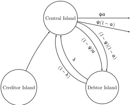
Creditors with a taste for domestic goods go directly to the domestic debtor’s islands and buy amount DA,Act+1 of the domestic good at price Pd,tA+1. Once the transactions have been made creditors then consume the debtor goods they bought. The total travel patterns as discussed in this section and section 3 are depicted in figure 3. In the first stage of travel all creditors andλ debtors arrive. Then α creditors leave early with ψ traveling to the foreign debtor is-lands and the remainder travel to the domestic debtor isis-lands. The remaining (1−λ) debtors arrive and settle their debt. The remaining (1−α) creditors then leave for debtor islands withψ traveling to the foreign debtor island and the remainder traveling to the domestic debtor island.
4.1
Creditors Maximization Problem
Country A creditors seek to maximize (2) subject to the timing frictions set out in sections 4 and 5. Therefore, their optimization programme becomes max qA t ,ℓAt (1−ψ)h(1−α) UCA ct, D A,A ct+1 +αUCA ct,D˜ A,A ct+1 i +ψαUCA ct,D˜ B,A ct+1 + ψ(1−α)hβUCA ct,Dˆ B,A ct+1 + (1−β) UCA ct, D B,A ct+1 io
Central Island Debtor Island Creditor Island (1 ) (1 ) (1 )(1 ) (1 )
Figure 3: Travel pattern for old creditors and debtors.
subject to the following budge constraints, one each equating the amount of money a creditor has and the nominal value of goods purchased.
PA c,tC A ct =P A c,tC¯ A t −ℓ A t , (7) Pd,tA+1D˜ A,A ct+1 =ρ A t+1(1−λ)ℓ A t +λℓ A t , (8) PA d,t+1D A,A ct+1 = (1−ρAt+1)qtA+ℓ A t, (9) PB d,t+1 ˜ et+1 ˜ DB,Act+1 = ρAt+1(1−λ)ℓ A t +λℓ A t , (10) PB d,t+1 ˜ et+1 ˆ DB,Act+1 = (1−ρA t+1)qAt +ℓ A t , (11) PB d,t+1 et+1 DB,Act+1 = (1−ρA t+1)qAt +ℓ A t , (12)
and the liquidity constraint (6) is assumed to hold
λℓAt =ρ A
t+1qAt . (13)
Here, the tildes represent amounts purchased if the creditor must leave the settlement island early, hats denote amounts bought by a creditor who is in the other foreign exchange market—the early foreign exchange market if a late-leaver and vice versa for an early-late-leaver—and lower-case letters denote amounts
effected by an aggregate default.
The terms in equation (11) involving the foreign exchange market are slightly different for the country B creditor. In their case, the maximization problem is max qB t ,ℓBt (1−ψ)h(1−α) UCB ct, D B,B ct+1 +αUCB ct,D˜ B,B ct+1 i + ψ(1−α) UCB ct, D B,B ct+1 +ψαhβUCB ct,Dˆ A,B ct+1 + (1−β) UCB ct,D˜ A,B ct+1 i (14) subject to the country B versions of equations (7) to (13)
PB c,tC B ct =P B c,tC¯ B t −ℓ B t Pd,tB+1D˜ B,B ct+1 =ρ B t+1(1−λ)ℓ B t +λℓ B t PB d,t+1D B,B ct+1 = (1−ρBt+1)qtB+ℓ B t ˜ et+1Pd,tA+1D˜ A,B ct+1 = ρBt+1(1−λ)ℓ B t +λℓ B t et+1Pd,tA+1Dˆ A,B ct+1 = ρB t+1(1−λ)ℓBt +λℓ B t et+1Pd,tA+1D A,B ct+1 = (1−ρBt+1)q B t +ℓ B t
and the liquidity constraint (6) is assumed to hold
λℓBt =ρ B t+1q
B
t . (15)
To avoid increasing the complexity of the notation even further, I define— using either equation (13) or equation (15) and the market-clearing condition equation (5)—the functions
κ(ρA t+1) = λ(1−ρA t+1) ρA t+1 + 1, (16)
as the “return” for late leaving creditors and
τ(ρA
t+1) =ρAt+1(1−λ) +λ, (17) as “return” for earlier-leaving creditors. Therefore, the nominal amount of money that an early-leaving creditor has when leaving the central island for their final destination is, for a countryA creditor, τ(ρA
t+1)ℓAt and a late-leaving
countryA creditor has the nominal amount κ(ρA t+1)ℓAt.
liq-uidity shortage, soρt+1 <1, then 0< τ(ρt+1)<1 with κ(ρt+1)>1. Second, if there is no liquidity shortage then bothτt+1(ρt+1) and κ(ρt+1) equal one. The first property shows how a liquidity shortage shifts wealth from early- to late-leavers, while the second shows that the wealth is equal only when no shortage exists.
Using the optimization problem (11) and the multipliers (16) and (17) the, rather long, first-order condition for country A creditors may be rewritten as
0 = U2CA ct,D˜ A,A ct U1CA ct,D˜ A,A ct τ(ρ A t+1)− PA d,t+1 PA c,t (1−ψ)αU1CA ct,D˜ A,A ct PA d,t+1 + U2CA ct, D A,A ct U1 CA ct, D A,A ct κ(ρ A t+1)− PA d,t+1 PA c,t (1−ψ)(1−α) U1CA ct, D A,A ct PA d,t+1 + U2CA ct, D B,A ct U1CA ct, D B,A ct et+1κ(ρ A t+1)− PB d,t+1 PA c,t ψ(1−α)(1−β) U1CA ct, D B,A ct PB d,t+1 + U2CA ct,Dˆ B,A ct U1CA ct,Dˆ B,A ct e˜t+1κ(ρ A t+1)− PB d,t+1 PA c,t ψ(1−α)βU1CA ct,Dˆ B,A ct PB d,t+1 + U2CA ct,D˜ B,A ct U1CA ct,D˜ B,A ct e˜t+1τ(ρ A t+1)− PB d,t+1 PA c,t ψαU1CA ct,D˜ B,A ct PB d,t+1 , (18)
while the countryB creditor’s first-order condition can be written as 0 = U2CB ct,D˜ B,B ct U1CB ct,D˜ B,B ct τ(ρ B t+1)− PB d,t+1 PB c,t (1−ψ)αU1CB ct,D˜ B,B ct PB d,t+1 + U2CB ct, D B,B ct U1 CB ct, D B,B ct κ(ρ B t+1)− PB d,t+1 PB c,t (1−ψ)(1−α) U1CB ct, D B,B ct PB d,t+1 + U2CB ct, D A,B ct U1CB ct, D A,B ct κ(ρB t+1) et+1 − P A d,t+1 PB c,t ψ(1−α) U1CB ct, D A,B ct PA d,t+1 + U2CA ct,Dˆ B,A ct U1CA ct,Dˆ B,A ct τ(ρB t+1) et+1 − P A d,t+1 PB c,t ψαβU1CB ct,Dˆ A,B ct PA d,t+1 + U2CA ct,D˜ B,A ct U1CA ct,D˜ B,A ct κ(ρB t+1) ˜ et+1 − P A d,t+1 PB c,t ψ(1−α) U1CB ct,D˜ A,B ct PA d,t+1 . (19)
These characterize the necessary and sufficient condition for the creditors’ op-timization problems. At the optimum, the terms in brackets individually equal zero, At the optimum, each bracketed term equates a marginal rate of substitu-tion to a price ratio subject to a “wedge” introduced by the settlement fricsubstitu-tion.2 Without a settlement friction,τ(ρA
t+1) andκ(ρAt+1) equal one, so equations (18) and (19) are then solved by equating marginal rates of substitution to price ratios as in the socially optimal case.
5
Foreign Exchange Market
The domestic creditors who emigrate to the foreign island meet the foreign creditors who immigrate and exchange domestic currency for foreign currency in a foreign exchange market. In a manner similar to Fujiki (2003), the foreign exchange market operates in two waves, which may be thought of as country
B’s morning and countryB’s afternoon.
As previously mentioned, the two economies are identical in all respects except for their time zone. This difference in time zone implies that the two economies have different trading hours and some agents who leave the central
2
These may be also thought of as equating the stochastic discount factor and return in the different states of the world to the price of consumption in that state of the world in terms of present consumption.
island early in one economy interact in the foreign exchange market with late-leavers from the other economy’s central island.
This difference in time zone is represented by the parameterβ, which varies from zero to one. The larger the value ofβ the more “out of sync” are the two economies in terms of their trading day. When β equals zero, both countries have the same trading hours and early creditors only meet with other early creditors. When β equals one, neither country is willing to trade when the other country is open for trade.
Because of this difference, (1−β) earlyB creditors meetβ late Acreditors, as well as the early A creditors, to trade currencies. In the afternoon, the difference in time zones causes β of the early B creditors and all the late domestic creditors to meet with only (1−β) late country A creditors to trade currencies.
Creditors on both sides exchange their domestic money for foreign money at a market-determined exchange rate. In the early foreign exchange market, the exchange rate, denoted ˜et+1, is determined by
(1−β)α τ(ρB t+1)ℓBt = ˜et+1 α τ(ρA t+1) +β(1−α)κ(ρAt+1) ℓA t. (20)
Similarly, the exchange rate for the late foreign exchange market, denotedet+1,
is determined using the market clearing equation
β α τ(ρB t+1) + (1−α)κ(ρBt+1) ℓB t =et+1(1−β) (1−α)κ(ρAt+1)ℓAt . (21)
From these equations it is obvious that the exchange rate will depend on the relative amounts of loans supplied in the two domestic markets.
6
Equilibrium
Here, I shall define an equilibrium where, for all periods, all three types of markets—good markets, money markets and debt markets—clear, the first-order conditions of all four types of agents are satisfied and where the amount of goods consumed is equal to the endowments. This is formalized in the following definition:
Definition 1 (Equilibrium). An equilibrium is a set of tuples of country A
quantity sequences
{DA,A,D˜A,A, DA,B,D˜A,B,DˆA,B, DA, CA, CA}∞
countryB quantity sequences {DB,Bct ,D˜ B,B ct , D B,A ct ,D˜ B,A ct ,Dˆ B,A ct , DdtB, CctB, CdtB} ∞ t=1, countryA price sequences
{Pc,tA, P A d,t}
∞
t=1, countryB price sequences
{PB c,t, P B d,t} ∞ t=1, countryA monetary and debt sequences
{mA t , ℓ A t, h A t} ∞ t=1, and countryB monetary and debt sequences
{mB t , ℓ B t , h B t } ∞ t=1 such that
1. Agents are maximizing utility, so equation (18) and equation (19) are satisfied for allt and equation (3.1) is satisfied for countryAdebtors and countryB debtors for all t.
2. Markets clear, goods markets ¯ DA t =D A dt+ (1−ψ)(1−α)D A,A ct + (1−ψ)αD˜ A,A ct +ψ(1−α) ˜D A,B ct +ψβαDˆA,Bct +ψ(1−α)D A,B ct ¯ DB t =D B dt+ (1−ψ)(1−α)D B,B ct + (1−ψ)αD˜ B,B ct +ψ(1−β)(1−α)D B,A ct +ψβ(1−α) ˆDctB,A+ψαD˜ B,A ct ¯ CA t =C A ct +C A dt ¯ CtB=C B ct +C B dt, loan markets, ℓAt =h A t ℓB t =h B t ,
money markets, hA t =m A t hBt =m B t ,
and the secondary debt markets,
qtA+1 =α(1−λ)ℓ
A t
qB
t+1 =α(1−λ)ℓBt ,
as well as the foreign exchange markets, equations (20) and (21).
To simplify analysis, I shall assume endowments are constant and equal in the two economies for all time periods. Therefore, it is natural to define a time-invariant market equilibrium. Thus, I define a stationary equilibrium as an equilibrium in which all variables do not depend on the time index.
In addition, to examine the key frictions in the model, I shall also assume the liquidity constraint (6) binds,α exceeds λ, and that β does not equal zero. In the case of the liquidity constraint holding, it follows from equations (5) and (6) that the equilibrium discount rateρt+1 follows:
ρA t+1 =
(1−α)λ
α(1−λ). (22)
Substituting equation (22) into the first-order condition (11) implies that the late-leaving creditors who travel internal to their economy have a higher con-sumption than early-leavers. This obtains because, in a liquidity-constrained equilibrium, debt resells at a discount, so ρA
t+1 is less then one.
Assuming, for the moment, that the money supply is constant and equal tom in both countries A and B and the liquidity constraint (6) binds implies some characteristics of a stationary equilibrium.
First, a binding liquidity constraint implies that for each country the dis-count rate is
ρA t =
λ(1−α)
α(1−λ). (23)
Since this has no time-specific or country-specific elements, it follows that
ρA t =ρ
B
without intervention on the part of the monetary authorities.
Second, as mentioned previously, the liquidity constraint implies that ρ
is less then one. This in turn implies that τ(ρ) < 1 < κ(ρ): early-leavers have a smaller share of money when they leave the central island. The per capita amount of money that early-leavers have isℓB
t /αorλℓAt/αdepending on
nationality. The late-leaver’s per capita amount of money is (1−λ)
(1−α)ℓ A t or (1−λ) (1−α)ℓ B t,
again depending on nationality.
Third, when β does not equal zero, the exchange rate appreciates over the day. The rate of appreciation when the liquidity constraint binds is
e ˜ e = [βατ(ρ) + (1−α)κ(ρ)]ℓB (1−β)(1−α)κ(ρ)ℓA [β(1−α)κ(ρ) +ατ(ρ)]ℓA (1−β)ατ(ρ)ℓB = (βλ+ (1−λ)) (β(1−λ) +λ) (1−β)2λ(1−λ) >1. (25) From the second and third points, it follows that agents from country B
who participate in the FX market have three possible levels ofA-money when they arrive at the country A debtor islands. Either they are early-leavers who participated in the early FX market, early-leavers who participate in the late FX market—that is β-leavers—or late-leavers who participate in the late FX market. It follows from the liquidity constraint that
τ(ρ) ˜
e > τ(ρ)
e . (26)
This occurs because ˜e is less than e by the liquidity constraint and the time-zone difference between countries. It also follows from the liquidity constraint that
κ(ρ)
e > τ(ρ)
e . (27)
Therefore, the β-leavers have the least amount of foreign exchange when they reach the country A debtor islands. At first glance, it may seem that the relative wealth of the early-leavers in the early FX market and the late-leavers in the late FX market is indeterminate since we may write this ratio as
κ(ρ)
τ(ρ) ˜
e
e (28)
where the first term is weakly greater than one and the second term is weakly less than one; therefore their product may greater or less then one. But, without intervention, these two terms are both determined by the liquidity constraint,
and the product of the two is equal to, after simplification, is
α[β(1−λ) +λ] [1 + (1−β)λ] (1−α)(1−β)2λ2
which is strictly greater than one. In the case of countryAagents, theβ-leavers are late-leavers, so equations (26) and (27) may be rewritten as
κ(ρ)e > τ(ρ)˜e
and
κ(ρ)e > κ(ρ)˜e.
In addition, the countryA version of equation (28) is
κ(ρ)
τ(ρ)
e
˜
e,
which is strictly greater than one since both terms in the product are greater then one.
7
Social Planner’s Problem
The solution to the social planner’s problem provides a benchmark against which to judge candidate equilibria. The social planner is assumed to have as an objective function the weighted average utilities of the four different agents in the economies. Therefore, the planner maximizes
(1−µB) V CB d, D B d +µBh(1−ψ)αUCB c ,D˜ B,B c + (1−ψ)(1−α) U CB c , D B,B c +ψαβUCB c ,Dˆ A,B c + (1−β)αψUCB c ,D˜ A,B c +ψ(1−α) U CB c , D A,B c i +(1−µA) V CdA, D A d +µAh(1−ψ)αUCcA,D˜ A,A c + (1−ψ)(1−α) U CcA, D A,A c +ψ(1−α)βUCA c ,DˆcB,A + (1−β)(1−α)ψU CA c , DcB,A +ψαUCA c ,D˜cB,A i (29)
subject to the resource constraints of the four distinct types of goods, assuming a constant endowment, (θA) C¯A=CA d +CcA (30) (θB) C¯B=CB c +C B d (31) (δA) D¯A=DAd + (1−ψ)αD˜ A,A c + (1−ψ)(1−α)D A,A c +ψα(1−β) ˜DA,B c +ψβαDˆ A,B c +ψ(1−α)D A,B c (32) (δB) D¯B=DBd + (1−ψ)αD˜ B,B c + (1−ψ)(1−α)D B,B c (33) +ψαD˜B,A c +ψβ(1−α) ˆD B,A c +ψ(1−β)(1−α)D B,A c (34)
Here, the Lagrange multipliers for the constraints are given in parentheses on the left.
The above constrained optimization problem yields the following results. First, the marginal rate of substitution between debtors and creditors who consume domestically for a given country should be equalized,
V1 CdB, DBd V2(CB d , DBd) = U1CB c ,D˜cB,B U2 CB c ,D˜ B,B c = U1CB c ,D˜cB,B U2 CB c ,D˜ B,B c . (35)
Second, the marginal rate of substitution for creditors, who consume foreign goods, should be equalized across the three possible outcomes of the foreign exchange market U1 CB c , DcA,B U2CB c , D A,B c = U1CB c ,DˆA,Bc U2CB c ,Dˆ A,B c = U1CB c ,D˜cA,B U2CB c ,D˜ A,B c . (36)
Third, the weighted marginal utility of same-origin debtor goods is equalized between the two types of creditors,
µAU2 CcA, D A,A c =µBU2 CcB, D A,B c , (37) and µBU2 CB c , DB,Bc =µAU2 CA c , DB,Ac , (38)
If the cross-derivative of creditors utility, U12(·,·), is zero, then it follows that when µB exceeds µA, DA,A
c is less than DcA,B and DcB,A is less than DcB,B
which in turn implies thatDA
constant, then the social planner’s allocation should also be constant through time.
The optimal solution to the social planner’s problem essentially involves relaxing to relax both types of timing frictions, both inter- and intra-country. In addition, the goods are then apportioned according to the social planner’s weights.
When µB equals µA, regardless of the cross-derivative’s sign, it follows that
the social planner collapses the problem into a classical general-equilibrium problem with two types, creditors and debtors, ignoring nationality.
8
Monetary Policy
First, assume just one Monetary Authority (MA) for both economies. This MA is assumed to have the same welfare function as the social planner (29).
The MA is assumed to be able to print both country A and country B
money costlessly. It can also intervene in both discount-loan markets as well as both periods of the foreign exchange market.
I shall focus on stationary equilibria and policies. This rules out policies where there is non-zero money growth between periods and where the MA holds stocks of either type of money.
Since the MA has the same objective function as the social planner, it is natural to see whether a single MA can achieve the social planner’s alloca-tion. As shown in section 7, the social planner’s allocation is defined as an allocation where the marginal rates of substitution for the two types of agents are equalized within a country and the marginal utilities of the three possi-ble outcomes from traveling to the other country are equalized, which implies that the three outcomes are equalized. Therefore, if the MA can achieve the same equalizations, then it follows that he will have maximized his objective function.3
From equation (3.1), the first order condition of a debtor, and the first order conditions for creditors, equations (18) and (19), it follows that, at the optimum
τ(ρt) =κ(ρt) = 1
for both countries and for allt.
3
It is true that this characterization does not completely capture the social planner’s solution. The social planner’s solution could, in fact, be attained by allowing initially non-stationary policies which converge to in finite time to a non-stationary equilibrium.
Relaxing the liquidity constraint can be achieved in a stationary equilibrium by having an elastic money supply in each settlement market as described in Freeman (1996). The MA implements this by purchasing the fraction (α−λ) of debt in both settlement markets. This relaxes the liquidity constraints (15) and (13), and the discount rates of debt rise to equal one. In the late part of the settlement market, the remaining debtors arrive and settle their debt; at this point the MA retires the money it receives from the discounted debt it purchases.
When the MA provides an elastic money supply in both domestic markets, it then follows that the early foreign exchange rate is
˜
e = (1−β)αℓ
B
[(1−β)α+β]ℓA (39)
and the late foreign exchange rate is
e = [(1−α) +βλ]ℓ
B
[(1−α) +βα−β]ℓA. (40)
To implement a stationary equilibrium, which achieves the social planner’s allocation, these two exchange rates must be equated. The single MA may equalize these exchange rates by printing country B currency and selling it in the early exchange market where it is relatively more valuable. The MA then sells the country B money it has acquired in the late FX market when it is relatively more valuable. In the early foreign exchange market, the MA issues (βℓA/ℓB) country B money and uses this to buy A money. This additional
liquidity causes the early foreign exchange rate to rise to (ℓB/ℓA). Once this
transaction is over, the MA is left holding β of A money. Using this, the MA intervenes on the A side of the late foreign exchange rate which causes the exchange rate to fall to (ℓA/ℓB).
This intervention has the result that (e/e˜) equals one, leaving the MA with no reserves between periods and hence not changing the money supplies or the price levels,so the policy is a stationary one. Since all timing frictions—both internal to the two countries as well as between the two countries—have been relaxed, it follows that the allocation associated with this policy is the social planner’s allocation.
8.1
Two Monetary Authorities
A natural next question is whether this policy is implementable in a stationary way by two MA authorities acting in a coordinated manner. The internal fric-tions can both be dealt with by the respective monetary authorities using their own currencies. Due to the timing structure of the model, only the countryB
MA is able to implement a stationary equilibrium with no intra-day apprecia-tion since B money must be created in the early foreign exchange market.
Therefore, in the cooperative case, the policies of the two MAs is as follows: countryA’s policy is to setρA
t equal to one for alltand conduct no intervention
in the foreign exchange markets; country B’s policy is to set ρB
t equal to one
for all t, sell (βℓA/ℓB) of B money in the early foreign exchange market and
sell theA money it receives, as a result of the intervention in the early market, in the late foreign exchange market.
9
Policy Interdependence
Now assume that each island has an independent monetary authority that wishes to maximize the welfare of the inhabitants of its island chain. Each MA seeks to maximize the utility of their own debtor and creditor population given the policy choices of the MA of the other country. Therefore, the country A
MA has a welfare function of the form (1−µA) V CdA, D A d +µAh(1−ψ)αUCcA,D˜ A,A c +(1−ψ)(1−α) U CA c , D A,A c +ψ(1−α)βUCA c ,Dˆ B,A c +(1−β)(1−α)ψU CA c , D B,A c +ψαUCA c ,D˜ B,A c i (41)
whereµis the weight that the monetary authority places on the welfare of the debtors. CountryB’s MA has a welfare function which is similar in form,
(1−µB) V CdB, D B d +µBh(1−ψ)αUCcB,D˜ B,B c +(1−ψ)(1−α) U CB c , DB,Bc +ψαβUCB c ,DˆcA,B +(1−β)αψUCB c ,D˜ A,B c +ψ(1−α) U CB c , D A,B c i (42)
the natural difference being that the utility functions of the B creditor and debtor enter the welfare function of the countryB MA instead of theAcreditor and debtors.
Each monetary authority can costlessly print a unique unfalsifiable type of money. Each MA is able to transact in their own discount loan market and in both periods of the foreign exchange market. In addition, each MA can hold foreign reserves of the other’s currency between periods.
The policies employed by the two MAs form a non-cooperative game. In the remainder of the paper I will examine Nash equilibria defined as follows:
Definition 2 (Nash Policy Equilibrium). I define a Nash Policy Equilibrium
as a market equilibrium with a sequence of policy variables
{ρAt, ρ B t , υ A t , υ B t , m A t , m B t } ∞ t=1, (43) where υA
t and υBt are country A and country B’s MAs’ interventions in the
FX market such that an MA’s choice of policy sequences under their control maximize either their domestic welfare function, either (41) or (42), subject to the chosen policy sequence of the other MA.
A stationary Nash policy equilibrium is then a Nash policy equilibrium which is also a stationary equilibrium and where all policy variables are time invariant. The definition of stationarity implies that money growth must be zero for all t.
I shall further assume that there is a commitment technology which allows both MA to commit at time 0 to play a constant policy every period.4 There-fore, in a stationary equilibrium, each MA plays as a strategy a tuple consisting of a within period of intervention in the FX market (υA orυA), and a discount
rate (ρA, and ρB).
Showing that a two-monetary-authority system cannot maintain the social planner’s allocation proceeds from the fact that there is a constant amount of the four goods to divide between the four types of agents. The consumption of creditor goods is purely a domestic matter while a country’s domestic debtor goods are consumed by three of the four agents. In a stationary equilibrium, the monetary value, and real value due to stationarity, of foreign debtor goods that a foreign consuming creditor receives is a constant fraction of the foreign creditor’s supply of loans. The domestic MA takes this foreign loan amount as given and therefore does not internalize the effect that its own agent’s loan choice has on the other country’s agents.
4
the presence of an underlying market equilibrium makes it unclear whether the folk theorem can even be applied in a stationary Nash policy equilibrium.
The proof of this will proceed as follows. First, I shall present the solution to the problem where each MA chooses how to allocate the goods between do-mestic agents taking the amount of foreign goods available for redistribution as given. This optimization problem is subject to two sets of constraints: the first set limits the allocations an MA can choose from to those which are im-plementable by the loan market, the second set maps the amount that an MA chooses to allocate to domestic creditors to the amount of domestic good avail-able to the foreign MA for allocation among foreign creditors. Second, given an MA’s choice of domestic quantities and the policy variable choices of the foreign MA, I shall show that there is a market equilibrium which implements this allocation and a determinant set of domestic policy variables. Third, I shall then show that there is a joint indeterminacy of the policy variables which lead to the same quantity allocations.
First, consider the “partial” planner’s problem for each country. The partial planner allocates domestic goods between domestic agents prior to theψ shock being realized. The domestic goods allocated to foreign consuming creditors are then turned over to the other partial planner. The resulting foreign goods can then be distributed between domestic creditors who wish to consume foreign.
These restrictions are necessary to ensure that the possible market allo-cations are a subset of the given partial planner’s problem. In a stationary market equilibrium goods map one-to-one with the amount of money an agent has. The above restrictions on the partial planner mimic the timing of the foreign consumption shock. This restriction is without loss of generality for my purposes since all the possible market equilibria are in the choice set of the partial planner as well as non-market equilibria.
The optimization problem of the country A MA given these constraints, the resource constraints of the social planner, equations (30) to (33), and the welfare functions (41) and (42) is
max(1−µA) V CdA, D A d +µAh(1−ψ)αUCcA,D˜ A,A c +(1−ψ)(1−α) U CcA, D A,A c +ψ(1−α)βUCcA,Dˆ B,A c +(1−β)(1−α)ψU CA c , D B,A c +ψαUCA c ,D˜ B,A c i (44)
subject to (δa 1) C¯A =CdA+CcA, (45) (δ2a) ¯ DA=DdA+ (1−ψ)αD˜ A,A c + (1−ψ)(1−α)D A,A c + ψ[αD˜A,A c + (1−ψ)(1−α)D A,A c ] , (46) (δ3a) ψ[α ˜ DB,B c + (1−ψ)(1−α)D B,B c ] =ψαD˜ B,A c +ψβ(1−α) ˆD B,A c + (1−β)(1−α)DB,Ac . (47) The last terms in equation (46) are the amount ofA goods that are transferred to the other partial planner for redistribution amongst its agents. Similarly the left hand side of constraint (47) represents the amount of B debtor good that is transferred to theA partial planner’s control for redistribution.
Similarly the optimization problem for the B partial planner is max(1−µA) V CdB, D B d +µAh(1−ψ)αUCcB,D˜ B,B c +(1−ψ)(1−α) U CB c , DcB,B +ψ(1−α)βUCB c ,DˆA,Bc +(1−β)(1−α)ψU CB c , D A,B c +ψαUCB c ,D˜ A,B c i (48) subject to (δ1b) C¯B =CdB+C B c , (δb2) ¯ DB=DBd + (1−ψ)αD˜ B,B c + (1−ψ)(1−α)D B,B c + ψ[αD˜B,B c + (1−ψ)(1−α)D B,B c ], (49) (δb3) ψ[α ˜ DA,A c + (1−ψ)(1−α)D A,A c ] =ψα(1−β) ˜D A,B c +ψαβDˆ A,B c + ψ(1−α)DA,Bc ,
The game that the two MAs play therefore involves the allocation of quan-tities to domestic agents. The interdependence comes from the change this has on the constraints of the other partial planner. The existence of a Nash equilibrium follows from the fact that the quantities available to both MAs are finite and that the best response functions are continuous. The continuity of the best response functions follows from the fact that the value functions for the two above problems are continuous due to the continuity of the objective function and the compactness of the space of possible allocations.
the first-order conditions of the two optimization problems above. First, in a solution to the partial planner’s problem the internal liquidity shortage is eased by the domestic monetary authority. This is independent of the foreign partial planner’s problem. Second, the solution to the partial planner’s problem sets the marginal rate of substitution of the domestic consuming creditor with that of the domestic debtors. Third, the domestic MA will attempt to equalize the marginal utility of the three foreign consuming creditors, subject to the amount of foreign debtor goods made available in the foreign exchange market; the MA will not introduce more inequality of consumption.
In a Nash equilibrium the only thing that matters in a partial planner’s so-lution is the amount of debtor good apportioned to the creditors. This amount relaxes the other partial planner’s constraint of the other countries debtor goods that it can allocate to its consumers who have a ψ taste shock. In addition, it tightens the constraint on the amount of domestic goods allocated to do-mestic consuming creditors. Suppose a partial planner could allocate different quantities of domestic goods .
Using these facts and equating the marginal values of relaxing and tighten-ing the constraint on a given type of creditor good, yields
ψµAU2 CA c , DcA,A =µBU2 CB c , DcA,B , (50) and ψµBU2 CcB, D B,B c =µAU2 CcA, D B,A c , (51)
As can be seen by comparing equations (50) and (51) to (37) and (38)— of which the latter two are the necessary conditions for a social planner’s optimum—an equilibrium in the Nash policy sense, where equations (50) and (51) must hold, must be different from a social planner’s optimum where equa-tion (37) and (38) must hold.
From the above problems of the partial planners, one can see that an MAs policy is to set ρA and ρB equal to one, and as above in the single MA case
country B’s MA intervenes in the early FX market by the amount (βℓB/ℓA)
and reverses it in the later FX market.
The intuition behind the different allocations that arise from the social plan-ner’s allocation and the Nash policy allocation are similar to the intuition in Tapking and Yang (2006). One can think of both MAs as producers of settle-ment liquidity which the agents in the economy use to relax the coordination problem in the settlement market. For as Freeman (1996) pointed out, this
increases the amount of loans in equilibrium and allows more trade of goods. Since ex ante a creditor does not know whether they will consume domesti-cally or abroad it follows that, all other things being equal, an increase in the amount of loans in the foreign market will increase the return on accepting a check from a domestic debtor and therefore increase the domestic amount of checks in circulation. In the noncooporative case, an MA does not internalize this secondary effect an increase in domestic check writing (or alternatively an increase in the amount of debtor goods available to the creditors) has through increasing foreign check writing. Therefore, the settlement liquidity provided by the two MAs are complement goods and this complementarity is not fully taken into account by either MA.
The solution to a partial planner’s problem is equivalent to a market equilib-rium. This can be seen from the fact that the in a partial planner’s equilibrium the domestic consuming creditor’s and debtor’s marginal rates of substitution are equated to each other, which is a necessary condition for the market equilib-rium since that debtor’s marginal rate of substitution equals the price ratio in a market equilibrium. The resource constraints imply that the market clearing conditions for goods are satisfied. The constraints on the possible allocations of goods above replicate the constraints implied by the workings of the loan markets.
There is, however, an indeterminacy in the above policy: in a stationary, solution the money supply for both countries is constant between period. Each MA sets the intraday interest rate equal to one by using an elastic money supply in the settlement market. It expands the money supply by buying unsettled early debt and then decreases the money supply back to normal when he debt clears. The indeterminacy arises in the foreign exchange market. If countryB
increases the B money supply by more than the optimal amount above, then the MA of countryAcan increase its money supply by a compensating amount and uses the additional money to buy intervene in the foreign exchange markets. This will result in the same foreign exchange rates as above and, therefore, the same quantities will be allocated in the same manner. This indeterminacy is related to the indeterminacy of the foreign exchange rate found by Kareken and Wallace (1981). In this case, the exchange rate is determinant, but the policy used to achieve the exchange rate is partially indeterminate in terms of money supply levels.5
5
This does hold in a non-stationary equilibrium. There may exist equilibrium where changes in the money supply have real effects even though the relative supplies might be fixed. I thank Paula Hern´andez-Verme for this comment.
10
Conclusion
When agents use debt to facilitate trade, and there is uncertainty concerning the settlement of this debt, a central bank should provide liquidity to alleviate this uncertainty. In this paper, I have looked at the interaction between two central banks and whether they can reach the social optimum by a coordinated policy.
The model I constructed is an extension of Freeman (1996), the principle difference being that in my model, there exist two payment systems which have different times of operation. In addition, there is a separate authority in charge of each settlement system, each of which cares only for the participants belonging to its payment system.
In the non-cooperative case, I show that as a one-shot case the MA cannot implement the single MA case as an equilibrium. The non-cooperative result stems from the lack of choice in how creditors behave after extending the loans. While, in principle, this lack of choice is defensible as an extension of the current literature in payment systems—and has been argued to be one of the essential ingredients by Zhou (2000)—the strength of the results rests on these strong assumptions. Therefore, the natural next step in this line of research is to enrich the set of choices that creditors have to see what affect this has on the non-cooperative result.
References
Freeman, S.(1996): “The Payments System, Liquidity, and Rediscounting,”
American Economic Review, 86(5), 1126–1138.
Fujiki, H. (2003): “A Model of the Federal Reserve Act Under the Inter-national Gold Standard System,” Journal of Monetary Economics, 50(6), 1333–1350.
(2006): “Institutions of Foreign Exchange Settlement in a Two-Country Model,” Journal of Money Credit and Banking, 38(3), 697–719.
Hern´andez-Verme, P. (2005): “International Reserves Crises, Monetary Integration, and The Payments System During the International Gold Stan-dard,” Macroeconomic Dynamics, 9(4), 516–541.
Kareken, J., and N. Wallace (1981): “On the Indeterminacy of Equilib-rium Exchange Rates,” Quarterly Journal of Economics, 96(2), 207–222.
Martin, A.(2004): “Optimal Pricing of Intraday Liquidity,”Journal of Mon-etary Economics, 51(2), 401–424.
Melvin, M.(1995): International Money and Finance. Harper Collins College Publishers, New York, NY, fourth edn.
Tapking, J., and J. Yang (2006): “Horizontal and Vertical Intergration in Securities Trading and Settlement,” Journal of Money Credit and Banking, 38(7), 1765–1795.
Zhou, R. (2000): “Understanding Intraday Credit in Large-Value Payment Systems,” Federal Reserve Bank of Chicago Economic Perspectives, 24(3), 29–44.